Computer Tools for Bifurcation Analysis: General Approach with

More documents

Recommendations

Info

998 L. M. Pismen & B. Y. Rubinstein If it is required to derive the normal form for a single mode arising at a bifurcation point of the distributed system, one may use the call BifurcationTheory[operatoreqn, u, R, t, {r, dim}, spatscale, {U, U † }, amp, coef, eps, order, wavenumber, freq, opts]. Here r denotes a spatial variable (that can be a vector); dim is the space dimension and spatscale denotes an array consisting of the name of the spatial variable and its (integer) scaling exponent α. Finally, wavenumber must be set equal to zero for a long-scale instability and to some symbol in the short-scale case. In the latter case the wavevector needed for the calculations is generated automatically. The differentiation operators ∂/∂t and ∇ used in the operator equation operatoreqn are represented by the symbols Nabla[t] and Nabla[r], respectively. A more complicated form must be used in a case when there is an angular degeneracy of the normal modes, namely, when the different modes have the same values of their parameters but the wavevectors with equal lengths have different directions. It is rational to specify the mode data using the angular measurment for the wavevectors — BifurcationTheory[operatoreqn, u, R, t, {r, dim}, spatscale, {U, U † }, amps, coef, eps, order, wavenumber, freq, ampout, opts], where amps consists of the pairs {a j ,β j }with β j denoting an angle between the wavevector of the jth mode a j and some selected direction. If the argument ampout specifying the names of the amplitudes for which equations must be generated is omitted, equations for first amplitude only from the array amps would be produced. The most general form of the function is used for algebraically degenerated cases: BifurcationTheory[operatoreqn, u, R, t, {r, dim}, spatscale, amps, coef, eps, order, ampout, options] derives a set of amplitude equations for a distributed system of partial differential equations writteninanoperatorform.Hereamps is an array of elements specifying the normal modes appearing in the linear solution (57). Each item of amps is an array of six elements in the following order — amplitude of the mode (a j ), mode wavevector (k j ), time frequency (ω j ), eigenvector (U j ), eigenvector of the adjoint problem (U † j ),andorderofsmallness of the normal mode (d j ). ampout again denotes an array of the amplitude names for which the amplitude equations must be generated. 4. Amplitude Equations for Reaction–Diffusion Problems 4.1. Long-scale instabilities In this and the next subsections we present the result of derivation of the amplitude equations for reaction–diffusion problem (52) with capacitance matrix G equal to identity matrix I and diffusivity matrix D which does not depend on the bifurcation parameters. We start from the case where the instability domain is localized around k c = 0 restricting ourselves to nondegenerated nonresonant cases. The operator equation corresponding to the problem may be written as: DD.(Nabla[r] . Nabla[r])∗∗u + f[u, R] - Nabla[t]∗∗u == 0 where DD denotes the diffusivity matrix. Operator Nabla[r] is assumed to be vectorial, hence the scalar Laplacian is written as scalar product of two differential operators. The function is called as follows: BifurcationTheory[ DD.(Nabla[r].Nabla[r])**u + f[u,R] - Nabla[t]**u == 0, u, R, t, {r,2},{r,1},{U,Ut}, a, c, eps, 2, 0, 0] Unfortunately, the version 2.2.2 of Mathematica used in development of the package has no perfect typesetting abilities like the version 3.0. As a result the output of the function is very lengthy and is difficult to understand for the inexperienced user. Here and further, we present output produced by the function BifurcationTheory using standard textbook notation. The result produced by the function coincides with that of the monotonic bifurcation of the dynamical system (36) with the only exception — the Landau equation is converted into the Ginzburg– Landau equation with an additional diffusional term of the form: U † DU U † U (∇ 1∇ 1 )a. (63)
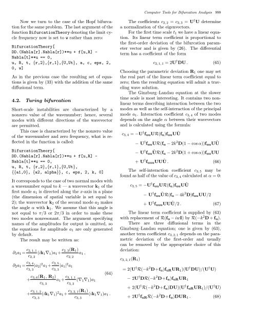
Computer Tools for Bifurcation Analysis 999 Now we turn to the case of the Hopf bifurcation for the same problem. The last argument of the function BifurcationTheory denoting the limit cycle frequency now is set to w rather than zero: BifurcationTheory[ DD.(Nabla[r].Nabla[r])**u + f[u,R] - Nabla[t]**u == 0, u, R, t, {r,2},{r,1},{U,Ut}, a, c, eps, 2, 0, w] As in the previous case the resulting set of equations is given by (33) with the addition of the same diffusional term. 4.2. Turing bifurcation Short-scale instabilities are characterized by a nonzero value of the wavenumber; hence, several modes with different directions of the wavevector are permitted. This case is characterized by the nonzero value of the wavenumber and zero frequency, what is reflected in the function is called: BifurcationTheory[ DD.(Nabla[r].Nabla[r])**u + f[u,R] - Nabla[t]**u == 0, u, R, t, {r,2},{r,1},{U,Ut}, {{a1,0}, {a2, alpha}}, c, eps, 2, k, 0] It corresponds to the case of two normal modes with awavenumberequaltok— a wavevector k 1 of the first mode a 1 is directed along the x-axis in a plane (the dimension of spatial variable is set equal to 2); the wavevector k 2 of the second mode a 2 makes the angle α with k 1 . We assume that this angle is not equal to π/3 or2π/3 inordertomakethese two modes nonresonant. The argument specifying names of the amplitudes for output is omitted, so the equations for amplitude a 1 are only generated by default. Theresultmaybewrittenas: ∂ 1 a 1 = c 2,1,1 c 2,2 (ik 1 ∇ 1 )a 1 + c 2,3(R 1 ) c 2,2 a 1 , ∂ 2 a 1 = c 3,4 c 3,3 |a 2 | 2 a 1 + c 3,5 c 3,3 |a 1 | 2 a 1 + c 3,6(R 1 ,R 2 ) c 3,3 a 1 + c 3,1,1 c 3,3 (∇ 1 ∇ 1 )a 1 (64) + c 3,1,2 c 3,3 (ik 1 ∇ 1 ) 2 a 1 + c 3,2,1(R 1 ) c 3,3 (ik 1 ∇ 1 )a 1 . The coefficients c 2, 2 = c 3, 3 = U † U determine a normalization of the eigenvectors. For the first time scale t 1 we have a linear equation. Its linear term coefficient is proportional to the first-order deviation of the bifurcation parameter vector and is given by (26). The differential term has a coefficient of the form c 2, 1, 1 =2U † DU . (65) Choosing the parametric deviation R 1 one may set the real part of the linear term coefficient equal to zero; then the resulting equation will admit a traveling wave solution. The Ginzburg–Landau equation at the slower time scale is most interesting. It contains two nonlinear terms describing interaction between the two modes as well as the self-interaction of the principal mode a 1 . Interaction coefficient c 3, 4 of two modes depends on the angle α between their wavevectors and is calculated using the formula: c 3, 4 = −U † f uu UR(f u )f uu UŨ − U † f uu UR(f u − 2k 2 D(1 − cos α))f uu UŨ − U † f uu ŨR(f u − 2k 2 D(1 + cos α))f uu UU + U † f uuu UUŨ . (66) The self-interaction coefficient c 3, 5 may be found as half of the value of c 3, 4 calculated at α =0: c 3,5 =−U † f uu UR(f u )f uu UŨ − U † f uu ŨR(f u − 4k 2 D)f uu UU/2 + U † f uuu UUŨ/2 . (67) The linear term coefficient is supplied by (63) with replacement of R(f u − iwI) byR(−k 2 D+f u ). There are three diffusional terms in the Ginzburg–Landau equation; one is given by (63), another term coefficient c 3, 2, 1 depends on the parametric deviation of the first-order and usually can be removed by the appropriate choice of this deviation: c 3, 2, 1 (R 1 ) =2(U † R(−k 2 D+f u )f uR UR 1 )(U † DU)/(U † U) − 2U † DR(−k 2 D+f u )f uR UR 1 +2(U † R(−k 2 D+f u )DU)(U † f uR UR 1 )/(U † U) +2U † f uR R(−k 2 D+f u )DUR 1 . (68)
Page 1 and 2: Tutorials and Reviews International
Page 3 and 4: Computer Tools for Bifurcation Anal
Page 15: Computer Tools for Bifurcation Anal
Page 21 and 22: There is also additional differenti

Computer Tools for Bifurcation Analysis: General Approach with

You also want an ePaper? Increase the reach of your titles

Delete template?

Save as template?