Computer Tools for Bifurcation Analysis: General Approach with

Computer Tools for Bifurcation Analysis 995
Now it is possible to compute the frequency
w = e y √ 0
y 0 − g 0 y 0 − 1/(1 + g 0 − y 0 )andtheeigenvectors:
{
g(1 − y0 − i √ }
y 0 − g 0 y 0 − 1)
U =
, 1 ;
y 0 (y 0 −1)
y0
4
3.5
3
super
sub
U † =
{
(y 0 − 1) g 0(1 − y 0 + i √ }
y 0 − g 0 y 0 − 1)
,1
1+g 0 −y 0
.
(48)
2.5
2
1.5
1
0.5
sub
As it was done above, one can choose the parametric
deviation of the first-order in such a way as
to make the first amplitude equation trivial. Then
the Landau coefficient in the second equation can
be presented after normalization as:
c 3, 2 /c 3, 1 =(y 0 −g 0 y 0 −1) 3/2 (iy 0 − i
− √ y 0 − g 0 y 0 − 1) −1 e y 0
/12
× (12 − 24g 0 − 24y 0 +40g 0 y 0 −4g 2 0 y 0
+14y 2 0−21g 0 y 2 0 +4g 2 0y 2 0 −2y 3 0 +2g 0 y 3 0
+i √ y 0 −g 0 y 0 −1(−12 + 24g 0 +15y 0
−25g 0 y 0 − 2g 2 0 y 0 − 5y 2 0 +8g 0y 2 0 )) . (49)
0 0.1 0.2 0.3 0.4 0.5 0.6 0.7
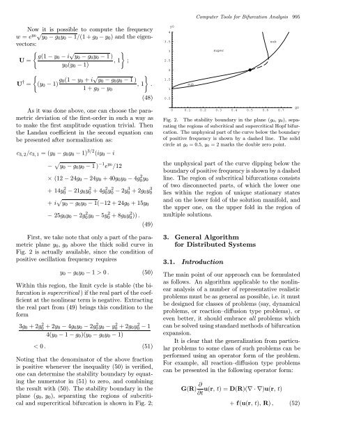
Fig. 2. The stability boundary in the plane (g 0,y 0), separating
the regions of subcritical and supercritical Hopf bifurcation.
The unphysical part of the curve below the boundary
of positive frequency is shown by a dashed line. The solid
circle at g 0 =0.5,y 0= 2 marks the double zero point.
the unphysical part of the curve dipping below the
boundary of positive frequency is shown by a dashed
line. The region of subcritical bifurcations consists
of two disconnected parts, of which the lower one
lies within the region of unique stationary states
and on the lower fold of the solution manifold, and
the upper one, on the upper fold in the region of
multiple solutions.
g0
First, we take note that only a part of the parametric
plane y 0 ,g 0 above the thick solid curve in
Fig. 2 is actually available, since the condition of
positive oscillation frequency requires
y 0 − g 0 y 0 − 1 > 0 . (50)
Within this region, the limit cycle is stable (the bifurcation
is supercritical ) if the real part of the coefficient
at the nonlinear term is negative. Extracting
the real part from (49) brings this condition to the
form
3g 0 +2g 2 0 +2y 0−4g 0 y 0 −2g 2 0 y 0−y 2 0 +2g 0y 2 0 −1
4(y 0 − 1 − g 0 )(y 0 − g 0 y 0 − 1)
< 0 . (51)
Noting that the denominator of the above fraction
is positive whenever the inequality (50) is verified,
one can determine the stability boundary by equating
the numerator in (51) to zero, and combining
the result with (50). The stability boundary in the
plane (g 0 ,y 0 ), separating the regions of subcritical
and supercritical bifurcation is shown in Fig. 2;
3. General Algorithm
for Distributed Systems
3.1. Introduction
The main point of our approach can be formulated
as follows. An algorithm applicable to the nonlinear
analysis of a number of representative realistic
problems must be as general as possible, i.e. it must
be designed for classes of problems (say, dynamical
problems, or reaction–diffusion type problems), or
even better, it should embrace all problems which
can be solved using standard methods of bifurcation
expansion.
It is clear that the generalization from particular
problems to some class of such problems can be
performed using an operator form of the problem.
For example, all reaction–diffusion type problems
can be presented in the following operator form:
G(R) ∂ u(r, t)=D(R)(∇·∇)u(r,t)
∂t
+f(u(r,t),R), (52)