Computer Tools for Bifurcation Analysis: General Approach with

1000 L. M. Pismen & B. Y. Rubinstein
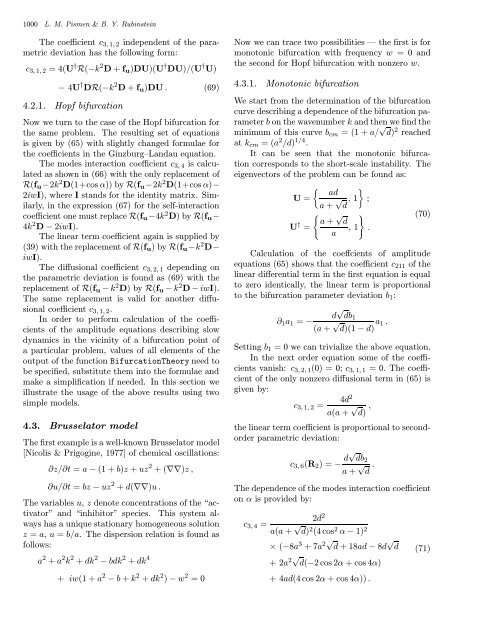
The coefficient c 3, 1, 2 independent of the parametric
deviation has the following form:
c 3, 1, 2 =4(U † R(−k 2 D+f u )DU)(U † DU)/(U † U)
− 4U † DR(−k 2 D + f u )DU . (69)
4.2.1. Hopf bifurcation
Now we turn to the case of the Hopf bifurcation for
the same problem. The resulting set of equations
is given by (65) with slightly changed formulae for
the coefficients in the Ginzburg–Landau equation.
The modes interaction coefficient c 3, 4 is calculated
as shown in (66) with the only replacement of
R(f u −2k 2 D(1+cos α)) by R(f u −2k 2 D(1+cos α)−
2iwI), where I stands for the identity matrix. Similarly,
in the expression (67) for the self-interaction
coefficient one must replace R(f u −4k 2 D)byR(f u −
4k 2 D−2iwI).
The linear term coefficient again is supplied by
(39) with the replacement of R(f u )byR(f u −k 2 D−
iwI).
The diffusional coefficient c 3, 2, 1 depending on
the parametric deviation is found as (69) with the
replacement of R(f u − k 2 D)byR(f u −k 2 D−iwI).
The same replacement is valid for another diffusional
coefficient c 3, 1, 2 .
In order to perform calculation of the coefficients
of the amplitude equations describing slow
dynamics in the vicinity of a bifurcation point of
a particular problem, values of all elements of the
output of the function BifurcationTheory need to
be specified, substitute them into the formulae and
make a simplification if needed. In this section we
illustrate the usage of the above results using two
simple models.
4.3. Brusselator model
The first example is a well-known Brusselator model
[Nicolis & Prigogine, 1977] of chemical oscillations:
∂z/∂t = a − (1 + b)z + uz 2 +(∇∇)z,
∂u/∂t = bz − uz 2 + d(∇∇)u.
The variables u, z denote concentrations of the “activator”
and “inhibitor” species. This system always
has a unique stationary homogeneous solution
z = a, u = b/a. The dispersion relation is found as
follows:
a 2 + a 2 k 2 + dk 2 − bdk 2 + dk 4
+ iw(1 + a 2 − b + k 2 + dk 2 ) − w 2 =0
Now we can trace two possibilities — the first is for
monotonic bifurcation with frequency w =0and
the second for Hopf bifurcation with nonzero w.
4.3.1. Monotonic bifurcation
We start from the determination of the bifurcation
curve describing a dependence of the bifurcation parameter
b on the wavenumber k and then we find the
minimum of this curve b cm =(1+a/ √ d) 2 reached
at k cm =(a 2 /d) 1/4 .
It can be seen that the monotonic bifurcation
corresponds to the short-scale instability. The
eigenvectors of the problem can be found as:
{ } ad
U =
a + √ d , 1 ;
{ √ }
(70)
a + d
U † = , 1 .
a
Calculation of the coeffcients of amplitude
equations (65) shows that the coefficient c 211 of the
linear differential term in the first equation is equal
to zero identically, the linear term is proportional
to the bifurcation parameter deviation b 1 :
d √ db 1
∂ 1 a 1 = −
(a + √ d)(1 − d) a 1 .
Setting b 1 = 0 we can trivialize the above equation.
In the next order equation some of the coefficients
vanish: c 3, 2, 1 (0) = 0; c 3, 1, 1 =0.The coefficient
of the only nonzero diffusional term in (65) is
given by:
4d 2
c 3, 1, 2 =
a(a + √ d) ,
the linear term coefficient is proportional to secondorder
parametric deviation:
c 3, 6 (R 2 )=− d√ db 2
a + √ d .
The dependence of the modes interaction coefficient
on α is provided by:
2d 2
c 3, 4 =
a(a + √ d) 2 (4 cos 2 α − 1) 2
× (−8a 3 +7a 2√ d+18ad − 8d √ d
+2a 2√ d(−2cos2α+cos4α)
+4ad(4 cos 2α +cos4α)) .
(71)