Computer Tools for Bifurcation Analysis: General Approach with

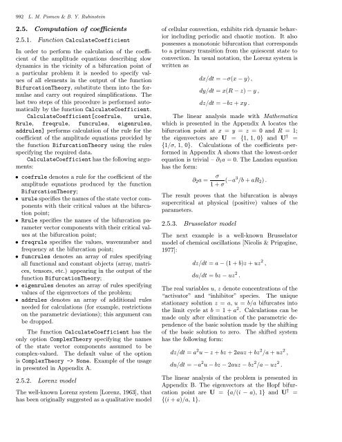
992 L. M. Pismen & B. Y. Rubinstein
2.5. Computation of coefficients
2.5.1. Function CalculateCoefficient
In order to perform the calculation of the coefficient
of the amplitude equations describing slow
dynamics in the vicinity of a bifurcation point of
a particular problem it is needed to specify values
of all elements in the output of the function
BifurcationTheory, substitute them into the formulae
and carry out required simplifications. The
last two steps of this procedure is performed automatically
by the function CalculateCoefficient.
CalculateCoefficient[coefrule, urule,
Rrule, freqrule, funcrules, eigenrules,
addrules] performs calculation of the rule for the
coefficient of the amplitude equations provided by
the function BifurcationTheory using the rules
specifying the required data.
CalculateCoefficient has the following arguments:
• coefrule denotes a rule for the coefficient of the
amplitude equations produced by the function
BifurcationTheory;
• urule specifies the names of the state vector components
with their critical values at the bifurcation
point;
• Rrule specifies the names of the bifurcation parameter
vector components with their critical values
at the bifurcation point;
• freqrule specifies the values, wavenumber and
frequency at the bifurcation point;
• funcrules denotes an array of rules specifying
all functional and constant objects (array, matrices,
tensors, etc.) appearing in the output of the
function BifurcationTheory;
• eigenrules denotes an array of rules specifying
values of the eigenvectors of the problem;
• addrules denotes an array of additional rules
needed for calculations (for example, restrictions
on the parametric deviations); this argument can
be dropped.
The function CalculateCoefficient has the
only option ComplexTheory specifying the names
of the state vector components assumed to be
complex-valued. The default value of the option
is ComplexTheory -> None. Example of the usage
in presented in Appendix A.
2.5.2. Lorenz model
The well-known Lorenz system [Lorenz, 1963], that
has been originally suggested as a qualitative model
of cellular convection, exhibits rich dynamic behavior
including periodic and chaotic motion. It also
possesses a monotonic bifurcation that corresponds
to a primary transition from the quiescent state to
convection. In usual notation, the Lorenz system is
written as
dx/dt = −σ(x − y) ,
dy/dt = x(R − z) − y,
dz/dt = −bz + xy .
The linear analysis made with Mathematica
which is presented in the Appendix A locates the
bifurcation point at x = y = z =0andR=1;
the eigenvectors are U = {1, 1, 0} and U † =
{1/σ, 1, 0}. Calculations of the coefficients performed
in Appendix A shows that the lowest-order
equation is trivial – ∂ 1 a =0.The Landau equation
has the form:
∂ 2 a =
σ
1+σ (−a3 /b + aR 2 ) .
The result proves that the bifurcation is always
supercritical at physical (positive) values of the
parameters.
2.5.3. Brusselator model
The next example is a well-known Brusselator
model of chemical oscillations [Nicolis & Prigogine,
1977]:
dz/dt = a − (1 + b)z + uz 2 ,
du/dt = bz − uz 2 .
The real variables u, z denote concentrations of the
“activator” and “inhibitor” species. The unique
stationary solution z = a, u = b/a bifurcates into
the limit cycle at b =1+a 2 . Calculations can be
made only after elimination of the parametric dependence
of the basic solution made by the shifting
of the basic solution to zero. The shifted system
has the following form:
dz/dt = a 2 u − z + bz +2auz + bz 2 /a + uz 2 ,
du/dt = −a 2 u − bz − 2auz − bz 2 /a − uz 2 .
The linear analysis of the problem is presented in
Appendix B. The eigenvectors at the Hopf bifurcation
point are U = {a/(i − a), 1} and U † =
{(i + a)/a, 1}.