Computer Tools for Bifurcation Analysis: General Approach with

Computer Tools for Bifurcation Analysis 1001
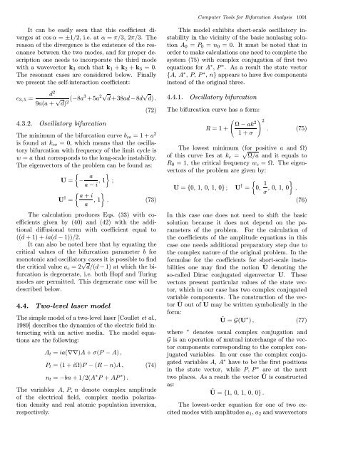
It can be easily seen that this coefficient diverges
at cos α = ±1/2, i.e. at α = π/3, 2π/3. The
reason of the divergence is the existence of the resonance
between the two modes, and for proper description
one needs to incorporate the third mode
with a wavevector k 3 such that k 1 + k 2 + k 3 =0.
The resonant cases are considered below. Finally
we present the self-interaction coefficient:
c 3, 5 =
d 2
9a(a + √ d) 2 (−8a3 +5a 2√ d+38ad−8d √ d) .
4.3.2. Oscillatory bifurcation
(72)
The minimum of the bifurcation curve b co =1+a 2
is found at k co = 0, which means that the oscillatory
bifurcation with frequency of the limit cycle is
w = a that corresponds to the long-scale instability.
The eigenvectors of the problem can be found as:
{
U = −
a }
a − i , 1 ;
U † =
{ a + i
a , 1 }
. (73)
The calculation produces Eqs. (33) with coefficients
given by (40) and (42) with the additional
diffusional term with coefficient equal to
((d +1)+ia(d − 1))/2.
It can also be noted here that by equating the
critical values of the bifurcation parameter b for
monotonic and oscillatory cases it is possible to find
the critical value a c =2 √ d/(d − 1) at which the bifurcation
is degenerate, i.e. both Hopf and Turing
modes are permitted. This degenerate case will be
described below.
4.4. Two-level laser model
The simple model of a two-level laser [Coullet et al.,
1989] describes the dynamics of the electric field interacting
with an active media. The model equations
are the following:
A t = ia(∇∇)A + σ(P − A) ,
P t =(1+iΩ)P − (R − n)A, (74)
n t = −bn +1/2(A ∗ P + AP ∗ ) .
The variables A, P, n denote complex amplitude
of the electrical field, complex media polarization
density and real atomic population inversion,
respectively.
This model exhibits short-scale oscillatory instability
in the vicinity of the basic nonlasing solution
A 0 = P 0 = n 0 = 0. It must be noted that in
order to make calculations one need to complete the
system (75) with complex conjugation of first two
equations for A ∗ ,P ∗ . As a result the state vector
{A, A ∗ ,P,P ∗ ,n}appears to have five components
instead of the original three.
4.4.1. Oscillatory bifurcation
The bifurcation curve has a form:
( )
Ω−ak
2 2
R =1+
. (75)
1+σ
The lowest minimum (for positive a and Ω)
of this curve lies at k c = √ Ω/a and it equals to
R 0 = 1, the critical frequency w c = Ω. The eigenvectors
of the problem are given by:
U = {0, 1, 0, 1, 0} ; U † =
{0, 1 }
σ , 0, 1, 0 .
(76)
In this case one does not need to shift the basic
solution because it does not depend on the parameters
of the problem. For the calculation of
the coefficients of the amplitude equations in this
case one needs additional preparatory step due to
the complex nature of the original problem. In the
formulae for the coefficients for short-scale instabilities
one may find the notion Ũ denoting the
so-called Dirac conjugated eigenvector U. These
vectors present particular values of the state vector,
which in our case has two complex conjugated
variable components. The construction of the vector
Ũ out of U may be written symbolically in the
form:
Ũ = G(U ∗ ) , (77)
where ∗ denotes usual complex conjugation and
G is an operation of mutual interchange of the vector
components corresponding to the complex conjugated
variables. In our case the complex conjugated
variables A, A ∗ have to be the first positions
in the state vector, while P, P ∗ are at the next
two places. As a result the vector Ũ is constructed
as:
Ũ = {1, 0, 1, 0, 0} .
The lowest-order equation for one of two excited
modes with amplitudes a 1 , a 2 and wavevectors