Computer Tools for Bifurcation Analysis: General Approach with
Computer Tools for Bifurcation Analysis: General Approach with
Computer Tools for Bifurcation Analysis: General Approach with

Create successful ePaper yourself
Turn your PDF publications into a flip-book with our unique Google optimized e-Paper software.
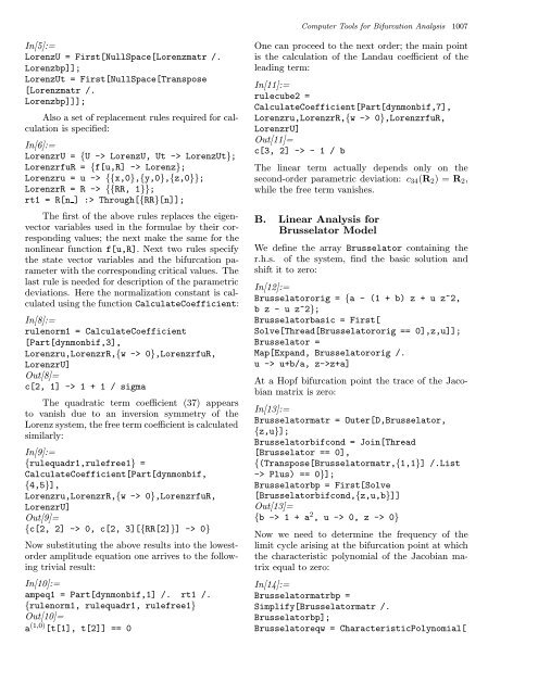
<strong>Computer</strong> <strong>Tools</strong> <strong>for</strong> <strong>Bifurcation</strong> <strong>Analysis</strong> 1007<br />
In[5]:=<br />
LorenzU = First[NullSpace[Lorenzmatr /.<br />
Lorenzbp]];<br />
LorenzUt = First[NullSpace[Transpose<br />
[Lorenzmatr /.<br />
Lorenzbp]]];<br />
Also a set of replacement rules required <strong>for</strong> calculation<br />
is specified:<br />
In[6]:=<br />
LorenzrU = {U -> LorenzU, Ut -> LorenzUt};<br />
LorenzrfuR = {f[u,R] -> Lorenz};<br />
Lorenzru = u -> {{x,0},{y,0},{z,0}};<br />
LorenzrR = R -> {{RR, 1}};<br />
rt1 = R[n ] :> Through[{RR}[n]];<br />
The first of the above rules replaces the eigenvector<br />
variables used in the <strong>for</strong>mulae by their corresponding<br />
values; the next make the same <strong>for</strong> the<br />
nonlinear function f[u,R]. Next two rules specify<br />
the state vector variables and the bifurcation parameter<br />
<strong>with</strong> the corresponding critical values. The<br />
last rule is needed <strong>for</strong> description of the parametric<br />
deviations. Here the normalization constant is calculated<br />
using the function CalculateCoefficient:<br />
In[8]:=<br />
rulenorm1 = CalculateCoefficient<br />
[Part[dynmonbif,3],<br />
Lorenzru,LorenzrR,{w ->0},LorenzrfuR,<br />
LorenzrU]<br />
Out[8]=<br />
c[2, 1] -> 1 + 1 / sigma<br />
The quadratic term coefficient (37) appears<br />
to vanish due to an inversion symmetry of the<br />
Lorenz system, the free term coefficient is calculated<br />
similarly:<br />
In[9]:=<br />
{rulequadr1,rulefree1} =<br />
CalculateCoefficient[Part[dynmonbif,<br />
{4,5}],<br />
Lorenzru,LorenzrR,{w ->0},LorenzrfuR,<br />
LorenzrU]<br />
Out[9]=<br />
{c[2, 2] -> 0, c[2, 3][{RR[2]}] -> 0}<br />
Now substituting the above results into the lowestorder<br />
amplitude equation one arrives to the following<br />
trivial result:<br />
In[10]:=<br />
ampeq1 = Part[dynmonbif,1] /. rt1 /.<br />
{rulenorm1, rulequadr1, rulefree1}<br />
Out[10]=<br />
a (1,0) [t[1], t[2]] == 0<br />
One can proceed to the next order; the main point<br />
is the calculation of the Landau coefficient of the<br />
leading term:<br />
In[11]:=<br />
rulecube2 =<br />
CalculateCoefficient[Part[dynmonbif,7],<br />
Lorenzru,LorenzrR,{w ->0},LorenzrfuR,<br />
LorenzrU]<br />
Out[11]=<br />
c[3, 2] -> - 1 / b<br />
The linear term actually depends only on the<br />
second-order parametric deviation: c 34 (R 2 )=R 2 ,<br />
while the free term vanishes.<br />
B. Linear <strong>Analysis</strong> <strong>for</strong><br />
Brusselator Model<br />
We define the array Brusselator containing the<br />
r.h.s. of the system, find the basic solution and<br />
shift it to zero:<br />
In[12]:=<br />
Brusselatororig = {a - (1 + b) z + u z^2,<br />
b z - u z^2};<br />
Brusselatorbasic = First[<br />
Solve[Thread[Brusselatororig == 0],z,u]];<br />
Brusselator =<br />
Map[Expand, Brusselatororig /.<br />
u -> u+b/a, z->z+a]<br />
At a Hopf bifurcation point the trace of the Jacobian<br />
matrix is zero:<br />
In[13]:=<br />
Brusselatormatr = Outer[D,Brusselator,<br />
{z,u}];<br />
Brusselatorbifcond = Join[Thread<br />
[Brusselator == 0],<br />
{(Transpose[Brusselatormatr,{1,1}] /.List<br />
-> Plus) == 0}];<br />
Brusselatorbp = First[Solve<br />
[Brusselatorbifcond,{z,u,b}]]<br />
Out[13]=<br />
{b -> 1 + a 2 , u -> 0, z -> 0}<br />
Now we need to determine the frequency of the<br />
limit cycle arising at the bifurcation point at which<br />
the characteristic polynomial of the Jacobian matrix<br />
equal to zero:<br />
In[14]:=<br />
Brusselatormatrbp =<br />
Simplify[Brusselatormatr /.<br />
Brusselatorbp];<br />
Brusselatoreqw = CharacteristicPolynomial[