Computer Tools for Bifurcation Analysis: General Approach with

998 L. M. Pismen & B. Y. Rubinstein
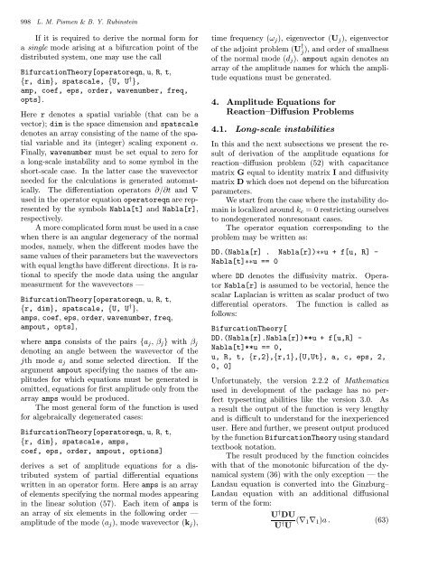
If it is required to derive the normal form for
a single mode arising at a bifurcation point of the
distributed system, one may use the call
BifurcationTheory[operatoreqn, u, R, t,
{r, dim}, spatscale, {U, U † },
amp, coef, eps, order, wavenumber, freq,
opts].
Here r denotes a spatial variable (that can be a
vector); dim is the space dimension and spatscale
denotes an array consisting of the name of the spatial
variable and its (integer) scaling exponent α.
Finally, wavenumber must be set equal to zero for
a long-scale instability and to some symbol in the
short-scale case. In the latter case the wavevector
needed for the calculations is generated automatically.
The differentiation operators ∂/∂t and ∇
used in the operator equation operatoreqn are represented
by the symbols Nabla[t] and Nabla[r],
respectively.
A more complicated form must be used in a case
when there is an angular degeneracy of the normal
modes, namely, when the different modes have the
same values of their parameters but the wavevectors
with equal lengths have different directions. It is rational
to specify the mode data using the angular
measurment for the wavevectors —
BifurcationTheory[operatoreqn, u, R, t,
{r, dim}, spatscale, {U, U † },
amps, coef, eps, order, wavenumber, freq,
ampout, opts],
where amps consists of the pairs {a j ,β j }with β j
denoting an angle between the wavevector of the
jth mode a j and some selected direction. If the
argument ampout specifying the names of the amplitudes
for which equations must be generated is
omitted, equations for first amplitude only from the
array amps would be produced.
The most general form of the function is used
for algebraically degenerated cases:
BifurcationTheory[operatoreqn, u, R, t,
{r, dim}, spatscale, amps,
coef, eps, order, ampout, options]
derives a set of amplitude equations for a distributed
system of partial differential equations
writteninanoperatorform.Hereamps is an array
of elements specifying the normal modes appearing
in the linear solution (57). Each item of amps is
an array of six elements in the following order —
amplitude of the mode (a j ), mode wavevector (k j ),
time frequency (ω j ), eigenvector (U j ), eigenvector
of the adjoint problem (U † j ),andorderofsmallness
of the normal mode (d j ). ampout again denotes an
array of the amplitude names for which the amplitude
equations must be generated.
4. Amplitude Equations for
Reaction–Diffusion Problems
4.1. Long-scale instabilities
In this and the next subsections we present the result
of derivation of the amplitude equations for
reaction–diffusion problem (52) with capacitance
matrix G equal to identity matrix I and diffusivity
matrix D which does not depend on the bifurcation
parameters.
We start from the case where the instability domain
is localized around k c = 0 restricting ourselves
to nondegenerated nonresonant cases.
The operator equation corresponding to the
problem may be written as:
DD.(Nabla[r] . Nabla[r])∗∗u + f[u, R] -
Nabla[t]∗∗u == 0
where DD denotes the diffusivity matrix. Operator
Nabla[r] is assumed to be vectorial, hence the
scalar Laplacian is written as scalar product of two
differential operators. The function is called as
follows:
BifurcationTheory[
DD.(Nabla[r].Nabla[r])**u + f[u,R] -
Nabla[t]**u == 0,
u, R, t, {r,2},{r,1},{U,Ut}, a, c, eps, 2,
0, 0]
Unfortunately, the version 2.2.2 of Mathematica
used in development of the package has no perfect
typesetting abilities like the version 3.0. As
a result the output of the function is very lengthy
and is difficult to understand for the inexperienced
user. Here and further, we present output produced
by the function BifurcationTheory using standard
textbook notation.
The result produced by the function coincides
with that of the monotonic bifurcation of the dynamical
system (36) with the only exception — the
Landau equation is converted into the Ginzburg–
Landau equation with an additional diffusional
term of the form:
U † DU
U † U (∇ 1∇ 1 )a. (63)