Total Beta Proponents Response to Eric Nath - BVMarketData
Total Beta Proponents Response to Eric Nath - BVMarketData
Total Beta Proponents Response to Eric Nath - BVMarketData

You also want an ePaper? Increase the reach of your titles
YUMPU automatically turns print PDFs into web optimized ePapers that Google loves.
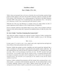
Letter <strong>to</strong> Edi<strong>to</strong>r<br />
This leter <strong>to</strong> the edi<strong>to</strong>r is in response <strong>to</strong> <strong>Eric</strong> W. <strong>Nath</strong>’s leter <strong>to</strong> the edi<strong>to</strong>r which was published on page<br />
51 in the Spring 2011 Business Valuation Review.<br />
In that letter, Mr. <strong>Nath</strong> shows a simple chart with two s<strong>to</strong>cks going in uniformly opposite directions. He<br />
correctly calculates the same standard deviation for both s<strong>to</strong>cks and, therefore, the same <strong>to</strong>tal beta<br />
equal <strong>to</strong> 1.2. He then states that,<br />
“This is just a general example of how there are, in fact, an infinite number of ways in<br />
which the standard deviation of returns for Company A and Company B could be<br />
identical, meaning identical <strong>Total</strong> <strong>Beta</strong>s, but with returns moving in completely opposite<br />
directions. <strong>Total</strong> <strong>Beta</strong> pays no attention <strong>to</strong> whether the prospects of a given company<br />
are positive or negative. <strong>Total</strong> <strong>Beta</strong> pays no attention <strong>to</strong> anything other than his<strong>to</strong>rical<br />
volatility, and is blind as <strong>to</strong> whether volatility in a particular case might be a good thing<br />
or a bad thing. How can anyone maintain with a straight face that the <strong>to</strong>tal risk of<br />
Company A and Company B are the same It looks <strong>to</strong> me like <strong>Total</strong> <strong>Beta</strong> cannot be true,<br />
but is simply a statistical non sequitur.”<br />
Mr. <strong>Nath</strong>’s aleged criticisms realy point <strong>to</strong> the CAPM (which almost al appraisers use in al<br />
assignments) as <strong>Total</strong> <strong>Beta</strong> is merely an extension of CAPM theory for undiversified inves<strong>to</strong>rs. For<br />
example, calculations of <strong>Beta</strong> are also based on his<strong>to</strong>rical s<strong>to</strong>ck prices. <strong>Beta</strong> calculations are also<br />
dependent upon the same relative standard deviations as <strong>Total</strong> <strong>Beta</strong>. Moreover, <strong>Beta</strong>s can equal each<br />
other, yet follow divergent paths.Is <strong>Beta</strong>, therefore, a statistical “non sequitur” Of course not.<br />
Ironically, Mr. <strong>Nath</strong> seems <strong>to</strong> criticize the use of his<strong>to</strong>ry yet likes his<strong>to</strong>ry <strong>to</strong> distinguish between alleged<br />
“good” and “bad” volatility <strong>to</strong> determine the prospects of a given company. What Mr. <strong>Nath</strong> has failed <strong>to</strong><br />
realize, however, is that according <strong>to</strong> modern portfolio theory (MPT) - ALL volatility is bad. Again, <strong>to</strong>tal<br />
beta applies MPT <strong>to</strong> undiversified inves<strong>to</strong>rs. It is really as simple as that. Naysayers should not hold<br />
<strong>Total</strong> <strong>Beta</strong> <strong>to</strong> a higher standard than CAPM <strong>Beta</strong>. For a more technical response <strong>to</strong> Mr. <strong>Nath</strong>’s incorrect<br />
criticisms, please see below.<br />
Let’s look at the folowing Chart of aleged “good” and “bad” volatility:<br />
1
In the Chart above, which appears very similar <strong>to</strong> the chart that Mr. <strong>Nath</strong> created, Company A or the<br />
aleged “good” volatility company has a his<strong>to</strong>rical beta of negative 0.31 (rounded). Visualy, we think<br />
you can see that it is negatively correlated with the S&P 500 or the market. For the aleged “bad”<br />
volatility company– Company B, as you might gues, the “bad” volatility company has a positive 0.31<br />
beta, the mirror-image of Company A.<br />
Before we addres Mr. <strong>Nath</strong>’specific statements above let’s develop an equation for the future price of<br />
a non-dividend paying s<strong>to</strong>ck. The equation below is the most common equation for s<strong>to</strong>ck price and is<br />
used in the Black-Scholes option pricing equation…<br />
S t = S 0 exp(( t + W t )<br />
S<strong>to</strong>ck price <strong>to</strong>day is S 0 and we want <strong>to</strong> forecast S t , which is s<strong>to</strong>ck price at some future time t. The Greek<br />
symbol, mu (represents the rate of return that we expect the s<strong>to</strong>ck <strong>to</strong> earn. In our case, this would<br />
be the discount rate that we used <strong>to</strong> price the s<strong>to</strong>ck at time zero (t = 0). The Greek symbol, sigma<br />
(represents expected volatility. In most cases, we use his<strong>to</strong>rical s<strong>to</strong>ck prices <strong>to</strong> measure sigma. The<br />
symbol W t is a Brownian motion with mean zero and variance t, and is the random variable that is the<br />
source of all risk.<br />
With our s<strong>to</strong>ck pricing equation in hand let’s isolateMr. <strong>Nath</strong>’s statements above…<br />
“This is just a general example of how there are, in fact, an infinite number of ways in which the standard<br />
deviation of returns for Company A and Company B could be identical, meaning identical <strong>Total</strong> <strong>Beta</strong>s, but<br />
with returns moving in completely opposite directions.”<br />
The statement above is correct. The expected value of W t is zero, which means that we expect the s<strong>to</strong>ck<br />
<strong>to</strong> earn the discount rate (over the time interval [0,t]. But note that the variance of W t is non-zero,<br />
which means that in all cases (noting that in continuous time W t will never equal zero) the s<strong>to</strong>ck will<br />
actually earn greater than the discount rate or less than the discount rate. At time zero looking forward<br />
we do not know the path that the s<strong>to</strong>ck will follow but from the s<strong>to</strong>ck price equation above we do know<br />
the possible paths and their attendant probabilities.<br />
“<strong>Total</strong> <strong>Beta</strong> pays no attention <strong>to</strong> whether the prospects of a given company are positive or negative.”<br />
The statement above is incorrect. If W t were not random then S t would be known with certainty and mu<br />
(would be the risk-free rate. The fact is that from the perspective of time zero looking forward we do<br />
not know the value of W t (i.e. risk) which is why the discount rate is greater than the risk-free rate. The<br />
mere fact that the discount rate is greater than the risk-free rate says that we don’t know whether the<br />
actual prospects for the company are positive or negative and this uncertainty is the reason why the<br />
equity risk premium (r m –r f ) is greater than zero. If the equity risk premium is a function of volatility,<br />
and volatility gives us the distribution of possible results (good and bad), then by definition the discount<br />
rate obtained via the CAPM (or <strong>Total</strong> <strong>Beta</strong>) takes in<strong>to</strong> account the probabilities of both positive and<br />
negative prospects for the company being valued.<br />
2
“<strong>Total</strong> <strong>Beta</strong> pays no attention <strong>to</strong> anything other than his<strong>to</strong>rical volatility, and is blind as <strong>to</strong> whether<br />
volatility in a particular case might be a good thing or a bad thing.”<br />
The statement above is also incorrect. Volatility from the perspective of time zero looking forward is<br />
always bad. The utility function for a risk-averse inves<strong>to</strong>r has a first derivative that is positive (more of a<br />
good is always better than less) and a second derivative that is negative (marginal utility is decreasing).<br />
Remember that from the perspective of time zero we deal in expectations because from our vantage<br />
point we do not know whether W t will be positive (we will earn a rate of return greater than the<br />
discount rate) or negative (we will earn a rate of return less than the discount rate). The utility function<br />
for a risk-averse inves<strong>to</strong>r says that the deleterious effects on utility from a negative W t outweighs the<br />
salubrious effects on utility from a positive W t , which again is why we have discount rates that are<br />
greater than the risk-free rate. Both the CAPM and <strong>Total</strong> <strong>Beta</strong> equations reflect the utility function of a<br />
risk-averse inves<strong>to</strong>r. The discount rate obtained via the CAPM (or <strong>Total</strong> <strong>Beta</strong>) by definition takes in<strong>to</strong><br />
account the expected utility from rates of return that are a lot greater than expected, a lot worse than<br />
expected, and everything in between.<br />
Note that how one measures expected volatility is at the discretion of the appraiser. If the appraiser has<br />
definite opinions as <strong>to</strong> expected future volatility then the appraiser may want <strong>to</strong> use that number. In<br />
absence of any definite opinions or insights ex-post volatility (based on his<strong>to</strong>rical prices) is often used as<br />
a proxy for ex-ante (future expected) volatility.<br />
“How can anyone maintain with a straight face that the <strong>to</strong>tal risk of Company A and Company B are the<br />
same”<br />
Given that from the perspective of time zero looking forward we do not know the future value of W t ,<br />
and from the risk-averse inves<strong>to</strong>r’s utility function that puts more weight on negative outcomesthan<br />
positive ones, we can say with a straight face that the risk of Company A and Company B are the same.<br />
From the vantage point of time zero we expect both companies <strong>to</strong> earn the discount rate. From that<br />
vantage point we don’t know if actual volatility wil be a “good thing” or a “bad thing” but we do know<br />
that since risk-averse inves<strong>to</strong>rs put more weight on negative outcomes than positive ones ex-ante<br />
volatility is always a bad thing. If this were not the case then all inves<strong>to</strong>rs would be risk-neutral and the<br />
expected return on all risky assets would be the risk-free rate.<br />
From our work as appraisers, where we generally price <strong>to</strong>tal risk as opposed <strong>to</strong> just systematic risk, and<br />
consistent with the classical definition of <strong>to</strong>tal risk which is the variance or uncertainty of returns:<br />
Yes, we can confidently state with a straight face that we will calculate the same <strong>to</strong>tal risk premium for<br />
both companies (<strong>to</strong> be used as proxies for our subject company) going in<strong>to</strong> the future equal <strong>to</strong>:<br />
<strong>Total</strong> cost of equity (TCOE) = risk-free rate + <strong>to</strong>tal beta*ERP<br />
TCOE = 5% + 1.2*6% = 12.2%<br />
Notice the rate is positive and greater than the risk-free rate. Whether or not we use 12.2% for our<br />
subject company is another question and that depends on our assessment of its relative risk when<br />
3
compared <strong>to</strong> both companies. This is where <strong>Total</strong> <strong>Beta</strong> beats other costs of capital models hands down<br />
–at least in our opinion. We now have–on a <strong>to</strong>tal risk perspective–both quantitative (think operating<br />
results over time) and qualitative disclosure of risks (think reading Forms 10-K) on multiple specific<br />
benchmarks <strong>to</strong> better support our determination of the appropriate discount rate. With these <strong>to</strong>ols at<br />
our disposal, most of the time, we feel we can explain the observed volatility in a s<strong>to</strong>ck. Moreover, <strong>Total</strong><br />
<strong>Beta</strong>s are generally more stable across time than <strong>Beta</strong>s, which is principally due <strong>to</strong> the volatility of the<br />
correlation coefficient. This is another huge advantage that <strong>Total</strong> <strong>Beta</strong> has over merely using <strong>Beta</strong> <strong>to</strong><br />
develop a discount rate for private companies.<br />
In any event, what rate of return would you use for your subject company, Mr. <strong>Nath</strong>, assuming you used<br />
these two companies as proxies Please tell us how you would arrive at your conclusion<br />
For what it is worth, we worked with Mr. <strong>Nath</strong>’s unlikely example because that is the hypothetical he<br />
gave <strong>Total</strong> <strong>Beta</strong> proponents. We believe, however, it shows that using very extreme and unlikely<br />
examples can provide aleged “evidence” for whatever one is trying <strong>to</strong> prove, especially when<br />
disregarding the realities of the marketplace and MPT.<br />
Finally, if Mr. <strong>Nath</strong> can tell us–with certainty based on his<strong>to</strong>rical s<strong>to</strong>ck prices - which one will provide a<br />
better return from an investment standpoint, we would like <strong>to</strong> hear it and encourage him <strong>to</strong> enter the<br />
investment management profession.<br />
Respectfully submitted,<br />
Peter J. Butler, CFA, ASA<br />
Gary S. Schurman, CFA, CPA<br />
4