A Study of Value-Based Branch Prediction Techniques
A Study of Value-Based Branch Prediction Techniques
A Study of Value-Based Branch Prediction Techniques

Create successful ePaper yourself
Turn your PDF publications into a flip-book with our unique Google optimized e-Paper software.
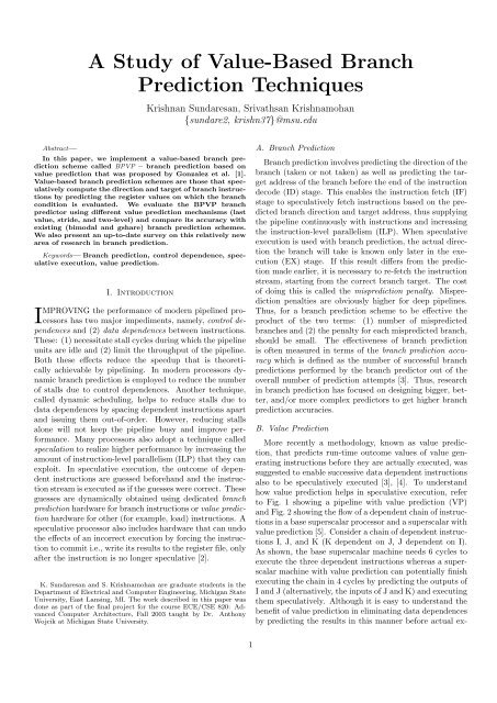
A <strong>Study</strong> <strong>of</strong> <strong>Value</strong>-<strong>Based</strong> <strong>Branch</strong><br />
<strong>Prediction</strong> <strong>Techniques</strong><br />
Krishnan Sundaresan, Srivathsan Krishnamohan<br />
{sundare2, krishn37}@msu.edu<br />
Abstract—<br />
In this paper, we implement a value-based branch prediction<br />
scheme called BPVP – branch prediction based on<br />
value prediction that was proposed by Gonzalez et al. [1].<br />
<strong>Value</strong>-based branch prediction schemes are those that speculatively<br />
compute the direction and target <strong>of</strong> branch instructions<br />
by predicting the register values on which the branch<br />
condition is evaluated. We evaluate the BPVP branch<br />
predictor using different value prediction mechanisms (last<br />
value, stride, and two-level) and compare its accuracy with<br />
existing (bimodal and gshare) branch prediction schemes.<br />
We also present an up-to-date survey on this relatively new<br />
area <strong>of</strong> research in branch prediction.<br />
Keywords— <strong>Branch</strong> prediction, control dependence, speculative<br />
execution, value prediction.<br />
I. Introduction<br />
IMPROVING the performance <strong>of</strong> modern pipelined processors<br />
has two major impediments, namely, control dependences<br />
and (2) data dependences between instructions.<br />
These: (1) necessitate stall cycles during which the pipeline<br />
units are idle and (2) limit the throughput <strong>of</strong> the pipeline.<br />
Both these effects reduce the speedup that is theoretically<br />
achievable by pipelining. In modern processors dynamic<br />
branch prediction is employed to reduce the number<br />
<strong>of</strong> stalls due to control dependences. Another technique,<br />
called dynamic scheduling, helps to reduce stalls due to<br />
data dependences by spacing dependent instructions apart<br />
and issuing them out-<strong>of</strong>-order. However, reducing stalls<br />
alone will not keep the pipeline busy and improve performance.<br />
Many processors also adopt a technique called<br />
speculation to realize higher performance by increasing the<br />
amount <strong>of</strong> instruction-level parallelism (ILP) that they can<br />
exploit. In speculative execution, the outcome <strong>of</strong> dependent<br />
instructions are guessed beforehand and the instruction<br />
stream is executed as if the guesses were correct. These<br />
guesses are dynamically obtained using dedicated branch<br />
prediction hardware for branch instructions or value prediction<br />
hardware for other (for example, load) instructions. A<br />
speculative processor also includes hardware that can undo<br />
the effects <strong>of</strong> an incorrect execution by forcing the instruction<br />
to commit i.e., write its results to the register file, only<br />
after the instruction is no longer speculative [2].<br />
K. Sundaresan and S. Krishnamohan are graduate students in the<br />
Department <strong>of</strong> Electrical and Computer Engineering, Michigan State<br />
University, East Lansing, MI. The work described in this paper was<br />
done as part <strong>of</strong> the final project for the course ECE/CSE 820: Advanced<br />
Computer Architecture, Fall 2003 taught by Dr. Anthony<br />
Wojcik at Michigan State University.<br />
A. <strong>Branch</strong> <strong>Prediction</strong><br />
<strong>Branch</strong> prediction involves predicting the direction <strong>of</strong> the<br />
branch (taken or not taken) as well as predicting the target<br />
address <strong>of</strong> the branch before the end <strong>of</strong> the instruction<br />
decode (ID) stage. This enables the instruction fetch (IF)<br />
stage to speculatively fetch instructions based on the predicted<br />
branch direction and target address, thus supplying<br />
the pipeline continuously with instructions and increasing<br />
the instruction-level parallelism (ILP). When speculative<br />
execution is used with branch prediction, the actual direction<br />
the branch will take is known only later in the execution<br />
(EX) stage. If this result differs from the prediction<br />
made earlier, it is necessary to re-fetch the instruction<br />
stream, starting from the correct branch target. The cost<br />
<strong>of</strong> doing this is called the misprediction penalty. Misprediction<br />
penalties are obviously higher for deep pipelines.<br />
Thus, for a branch prediction scheme to be effective the<br />
product <strong>of</strong> the two terms: (1) number <strong>of</strong> mispredicted<br />
branches and (2) the penalty for each mispredicted branch,<br />
should be small. The effectiveness <strong>of</strong> branch prediction<br />
is <strong>of</strong>ten measured in terms <strong>of</strong> the branch prediction accuracy<br />
which is defined as the number <strong>of</strong> successful branch<br />
predictions performed by the branch predictor out <strong>of</strong> the<br />
overall number <strong>of</strong> prediction attempts [3]. Thus, research<br />
in branch prediction has focused on designing bigger, better,<br />
and/or more complex predictors to get higher branch<br />
prediction accuracies.<br />
B. <strong>Value</strong> <strong>Prediction</strong><br />
More recently a methodology, known as value prediction,<br />
that predicts run-time outcome values <strong>of</strong> value generating<br />
instructions before they are actually executed, was<br />
suggested to enable successive data dependent instructions<br />
also to be speculatively executed [3], [4]. To understand<br />
how value prediction helps in speculative execution, refer<br />
to Fig. 1 showing a pipeline with value prediction (VP)<br />
and Fig. 2 showing the flow <strong>of</strong> a dependent chain <strong>of</strong> instructions<br />
in a base superscalar processor and a superscalar with<br />
value prediction [5]. Consider a chain <strong>of</strong> dependent instructions<br />
I, J, and K (K dependent on J, J dependent on I).<br />
As shown, the base superscalar machine needs 6 cycles to<br />
execute the three dependent instructions whereas a superscalar<br />
machine with value prediction can potentially finish<br />
executing the chain in 4 cycles by predicting the outputs <strong>of</strong><br />
I and J (alternatively, the inputs <strong>of</strong> J and K) and executing<br />
them speculatively. Although it is easy to understand the<br />
benefit <strong>of</strong> value prediction in eliminating data dependences<br />
by predicting the results in this manner before actual ex-<br />
1
ecution <strong>of</strong> the instructions takes place, it can also have<br />
an impact on branch prediction [5]. Using value prediction,<br />
a branch misprediction can be detected earlier in the<br />
pipeline; this way the machine can start executing the correct<br />
path sooner rather than doing wasted work executing<br />
the wrong path.<br />
FETCH<br />
PC<br />
VPT<br />
ACCESS<br />
DECODE<br />
&<br />
RENAME<br />
prediction<br />
ISSUE<br />
if mispredicted<br />
EXECUTE<br />
VERIFY<br />
COMMIT<br />
Fig. 1. Schematic <strong>of</strong> a 5-stage pipeline with value prediction<br />
that supports speculative execution.<br />
Pipeline<br />
Base Superscalar<br />
Stage 1 2 3 4 5 6<br />
Fetch I,J,K<br />
Decode I,J,K<br />
Execute I J K<br />
Commit I J K<br />
Pipeline<br />
Superscalar with VP<br />
Stage 1 2 3 4<br />
Fetch<br />
I,J,K<br />
Decode<br />
I,J,K<br />
Execute<br />
I,J,K<br />
Commit<br />
I,J,K<br />
Fig. 2. Flow diagrams for a 5-stage pipeline in (i) base superscalar<br />
machine and (ii) base superscalar with value prediction.<br />
The base superscalar machine needs 6 cycles to execute<br />
the three dependent instructions whereas a superscalar machine with<br />
value prediction can execute it in 4 cycles.<br />
C. <strong>Value</strong>-based <strong>Branch</strong> <strong>Prediction</strong><br />
By combining the concepts <strong>of</strong> value prediction and<br />
branch prediction, a new class <strong>of</strong> branch prediction schemes<br />
called value-based branch prediction 1 schemes have been<br />
proposed recently [7], [8], [1], [6]. In this class <strong>of</strong> branch<br />
prediction schemes, the branch predictor is aided by some<br />
form <strong>of</strong> data value history <strong>of</strong> the branch register operands<br />
in addition to branch history. Two approaches for improving<br />
branch prediction using value-based approaches have<br />
been described by Heil et al. [8]. These are (i) the speculative<br />
branch execution approach and (ii) the branch prediction<br />
by correlating on data values approach. Fig. 3 shows<br />
schematic diagrams for the two approaches.<br />
• In the speculative branch execution approach, a conventional<br />
data (value) predictor is used to predict input values<br />
for branch instructions. Then the branch is evaluated using<br />
the predicted values. At the same time, a branch prediction<br />
is also obtained using conventional branch predictors.<br />
A chooser or selector is then used to select the final prediction.<br />
1 The term ’value-based branch prediction’ appears to have been<br />
first used by Chen et al. [6]. In this paper, we use it to encompass a<br />
variety <strong>of</strong> schemes that use value history for branch prediction.<br />
GLOBAL<br />
BRANCH<br />
HISTORY<br />
BRANCH PC<br />
DATA<br />
VALUE<br />
HISTORY<br />
CHOOSER<br />
BRANCH<br />
PRED.<br />
VALUE<br />
PRED.<br />
(a)<br />
BRANCH<br />
EXECUTION<br />
GLOBAL<br />
BRANCH<br />
HISTORY<br />
BRANCH PC<br />
DATA<br />
VALUE<br />
HISTORY<br />
(b)<br />
BRANCH<br />
PRED.<br />
Fig. 3. Two approaches to value-based branch prediction<br />
schemes proposed by Heil et al.: (a) speculative branch execution<br />
approach (b) branch prediction by correlating on data values<br />
approach.<br />
• In the second approach, the data value history is directly<br />
fed into the branch predictor. This enables the branch<br />
predictor to correlate on data values similar to the way it<br />
would correlate on global branch history.<br />
C.1 Potential <strong>of</strong> value-based branch prediction<br />
As mentioned earlier, value predictability has been studied<br />
by many authors [3], [4], [9]. Sazeides and Smith have<br />
evaluated the effect <strong>of</strong> value predictability on branch predictability<br />
[10]. Their evaluations show that many (up<br />
to 82%) <strong>of</strong> the branch nodes propagate predictability, i.e.,<br />
when the branch output is predictable, at least one <strong>of</strong> their<br />
inputs is also predictable. Another interesting result presented<br />
in their study is that branch mispredictions are rare<br />
even for branches with both unpredictable inputs and only<br />
about 50% <strong>of</strong> the branches are mispredicted when both inputs<br />
are predictable. Their study concludes that there is<br />
substantial potential for improving branch prediction accuracy<br />
by incorporating data value history information into<br />
existing branch predictors.<br />
C.2 Some pros and cons <strong>of</strong> value-based branch prediction<br />
One <strong>of</strong> the most important benefits <strong>of</strong> value-based branch<br />
prediction is that, as mentioned earlier, a branch misprediction<br />
can be detected earlier in the pipeline and the machine<br />
can start executing the correct path sooner. This<br />
can potentially reduce the amount <strong>of</strong> wasted work due to<br />
mispredictions. <strong>Value</strong>-based predictors are most useful in<br />
situations where other correlating predictors may fail, for<br />
example, while predicting branches at the end <strong>of</strong> large ’for’<br />
loops in programs. In such cases (when the number <strong>of</strong> loop<br />
iterations is greater than the history length <strong>of</strong> the correlating<br />
predictor), value based predictors can correctly predict<br />
the branches since the input <strong>of</strong> such branches will follow a<br />
well-defined stride pattern [1].<br />
However, if not carefully used, value-based branch predictors<br />
may potentially result in more mispredictions<br />
and/or delay branch resolution [5]. In value-based branch<br />
prediction, branches with speculative operands can be handled<br />
in two ways: (1) they are resolved when their operands<br />
are still speculative and (2) they are resolved only when<br />
their operands become non-speculative. The first option<br />
can increase the number <strong>of</strong> branch mispredictions since the<br />
predicted inputs may themselves be wrong. The second option<br />
forces the branch resolution to be postponed until after<br />
its producer instructions have been committed thus in-<br />
2
creasing the latency. Due to these drawbacks, most simple<br />
value-based branch prediction techniques have been used<br />
only in combination with other existing branch predictors<br />
[1]. However advanced value-based branch prediction techniques,<br />
that have been proposed recently using techniques<br />
such as dynamic data dependence tracking, have achieved<br />
higher accuracies when used independently [6].<br />
D. Contributions <strong>of</strong> this Work<br />
Gonzalez et al. have proposed a value-based branch prediction<br />
scheme called BPVP – branch prediction based on<br />
value prediction [1]. Their scheme uses the speculative<br />
branch execution approach described above. They have<br />
shown that value prediction can improve the overall accuracy<br />
<strong>of</strong> branch prediction techniques by correcting predictions<br />
that are mispredicted by classical branch predictors<br />
like history-based or correlating predictors. This approach<br />
identifies the instructions that generate the inputs<br />
for branches, predicts their output values, uses this predicted<br />
inputs to determine the branch outcome, and speculatively<br />
executes the instruction stream past the branch<br />
instruction. The study <strong>of</strong> value-based branch prediction<br />
schemes and the implementation and evaluation <strong>of</strong> the<br />
BPVP scheme is the focus <strong>of</strong> this paper. We focus on implementing<br />
the baseline BPVP scheme and use three different<br />
data value predictors, namely, last value, stride, and twolevel<br />
predictors in the BPVP implementation. We simulate<br />
these configurations and compare the prediction accuracy<br />
with respect to two classical branch predictors, bimodal<br />
and Gshare.<br />
The organization <strong>of</strong> the rest <strong>of</strong> this paper is as follows.<br />
In Sec. II, we present related work in the area <strong>of</strong><br />
branch prediction and value prediction techniques. Then<br />
in Sec. III, we describe the current state-<strong>of</strong>-the-art in value<br />
based branch prediction. Next in Sec. IV, we present details<br />
<strong>of</strong> our simulation environment and discuss briefly how<br />
we implemented the BPVP branch predictor. Then, we<br />
present simulation results and discussions in Sec. V and<br />
finally, we conclude in Sec. VI.<br />
II. Related Work<br />
In this section, we review the design <strong>of</strong> some popular<br />
branch prediction and value prediction schemes. Later in<br />
Sec. V, we will compare the performance <strong>of</strong> these schemes<br />
with the BPVP scheme.<br />
A. <strong>Branch</strong> <strong>Prediction</strong> Schemes<br />
We briefly review some popular branch prediction<br />
schemes below. For the interested reader, a survey <strong>of</strong><br />
branch prediction strategies can be found in [11].<br />
A.1 Static <strong>Branch</strong> <strong>Prediction</strong> Schemes<br />
Most branches exhibit a high degree <strong>of</strong> correlation with<br />
their past behavior and that <strong>of</strong> other branches in the vicinity.<br />
This correlation can be used to predict the outcome <strong>of</strong><br />
a branch in the decode stage to a high degree <strong>of</strong> accuracy<br />
(low miss prediction rate). This significantly reduces the<br />
overhead associated with branches. There are two methods<br />
one can use to statistically predict branches: (1) by examining<br />
the program behavior (branch direction, etc.) or (2)<br />
by the use <strong>of</strong> pr<strong>of</strong>ile information collected from earlier runs<br />
<strong>of</strong> the program (branch behaviors are <strong>of</strong>ten bimodally distributed,<br />
i.e., an individual branch is <strong>of</strong>ten highly biased<br />
toward taken or not-taken).<br />
A.2 Dynamic <strong>Branch</strong> <strong>Prediction</strong> Schemes<br />
Unlike static branch prediction schemes, dynamic branch<br />
prediction is implemented in hardware and the prediction<br />
can change if the branches change behavior while the<br />
program is running. Some popular examples <strong>of</strong> dynamic<br />
branch prediction schemes are discussed below.<br />
• One-bit Scheme: The simplest scheme is the branch prediction<br />
buffer (BPB) or branch history table (BHT). A<br />
branch prediction buffer (BPB) is a small memory indexed<br />
by the lower portion <strong>of</strong> the address <strong>of</strong> the branch instruction.<br />
The memory contains a bit that indicates whether<br />
the branch was recently taken or not. The downside <strong>of</strong> using<br />
a single bit is that even if a branch is almost always<br />
taken, it will likely be predicted incorrectly twice, rather<br />
than once, when it is not taken.<br />
• Two-bit prediction scheme[11]: The two-bit prediction<br />
scheme is also <strong>of</strong>ten called the bimodal branch predictor.<br />
It is known that most branches are either usually taken or<br />
usually not taken. Bimodal branch prediction takes advantage<br />
<strong>of</strong> this bimodal distribution <strong>of</strong> branch behavior and attempts<br />
to distinguish usually taken from usually not taken<br />
branches. It makes a prediction based on the direction that<br />
the branch went the last few times it was executed. The<br />
bimodal scheme uses a table <strong>of</strong> 2-bit saturating up-down<br />
counters to keep track <strong>of</strong> the direction a branch is more<br />
likely to take. Each branch is mapped via its address to<br />
a counter. The branch is predicted taken if the most significant<br />
bit <strong>of</strong> the associated counter is set; otherwise, it is<br />
predicted not taken. These counters are updated based on<br />
the branch outcomes. When a branch is taken, the 2-bit<br />
value <strong>of</strong> the associated saturating counter is incremented<br />
by one; otherwise, the value is decremented by one.<br />
• Two-level prediction scheme (Gshare)[12]: The two-bit<br />
predictor schemes use only the recent behavior <strong>of</strong> a branch<br />
to predict the future behavior <strong>of</strong> that branch. It may be<br />
possible to improve the prediction accuracy if we also look<br />
at the recent behavior <strong>of</strong> other branches rather than just<br />
the branch we are trying to predict. Hence predictors that<br />
use global branch history are called also correlating predictors.<br />
The Gshare predictor is a variation <strong>of</strong> the twolevel<br />
GAg/GAs global history predictor. Two-level prediction<br />
uses two tables: a pattern history table (PHT) at the<br />
lower level and a table <strong>of</strong> 2-bit predictors just like the bimodal<br />
described above. The idea is to use something other<br />
than the branch PC to index into the table <strong>of</strong> 2-bit predictors.<br />
In the Gshare configuration, the two-level predictor<br />
keeps 1 entry <strong>of</strong> hist-size bits <strong>of</strong> branch history in a global<br />
branch history register (GBHR), but it XORs those bits<br />
with hist-size bits taken from the PC before indexing into<br />
the second-level table to get the prediction. The advantage<br />
<strong>of</strong> using global history is that it can detect and pre-<br />
3
dict sequences <strong>of</strong> correlated branches. Also combining the<br />
stored branch history and branch PC (like the XOR done in<br />
Gshare) provides some degree <strong>of</strong> anti-aliasing and prevents<br />
conflict when indexing into the PHT. A 16K-entry Gshare<br />
predictor in which 12-bits <strong>of</strong> history are XORed with 14<br />
bits <strong>of</strong> branch PC is used in the Sun UltraSPARC-III processor.<br />
B. <strong>Value</strong> <strong>Prediction</strong> Schemes<br />
Data value prediction schemes predict the value <strong>of</strong> the<br />
result register in data-producing instructions based on past<br />
behavior. This is similar in some respects to branch prediction<br />
techniques, where the branch direction and the target<br />
address are predicted for speculative execution. But,<br />
data value prediction differs from branch prediction as it<br />
involves a multi-valued decision (i.e., an 1-out-<strong>of</strong>-2 w prediction,<br />
where w is the word size) as opposed to branch<br />
prediction which is a binary decision (i.e., an 1-out-<strong>of</strong>-2<br />
prediction) [13]. Below we present a review <strong>of</strong> three <strong>of</strong> the<br />
most commonly used data value prediction schemes.<br />
B.2 Stride Predictor<br />
Stride predictor uses data value locality by monitoring<br />
the stride by which consecutive instances <strong>of</strong> an instruction<br />
change. When the results <strong>of</strong> consecutive instances <strong>of</strong> an instruction<br />
change by a constant value, then the result <strong>of</strong> future<br />
instances can be predicted by storing the stride value.<br />
This can be easily observed in the behavior <strong>of</strong> loop induction<br />
variables and in programs stepping through arrays in<br />
a regular fashion. The block diagram <strong>of</strong> a stride-based predictor<br />
is shown in Fig. 5 [13]. It uses a VHT similar to last<br />
value predictor. But each entry in VHT has four fields:<br />
tag, state, value, and stride. The state field is necessary to<br />
detect stride pattern and to update/read the stride value.<br />
The stride predictor can be in one <strong>of</strong> 3 different states: init,<br />
transient, and steady.<br />
Fig. 5.<br />
Data value prediction schemes: Stride predictor<br />
Fig. 4.<br />
Data value prediction schemes: Last value predictor<br />
B.1 Last <strong>Value</strong> Predictor<br />
The simplest among data value prediction schemes is the<br />
last value predictor. Here, the result produced by an instruction<br />
the last time it was executed is stored and the<br />
same value is predicted when the instruction is executed<br />
again. The hardware structure used for last outcome or last<br />
value predictor is shown in Fig. 4 [13]. The basic idea is to<br />
store the output <strong>of</strong> all register write instructions. Since it<br />
is impossible, considering the hardware overhead required<br />
to store the outcome <strong>of</strong> all instances <strong>of</strong> every register write<br />
instruction, a hash function is used to do address mapping.<br />
The predictor uses a value history table (VHT) that<br />
stores the last value produced by the instructions mapped<br />
to it. Each VHT entry has two fields named tag and value.<br />
The tag field stores the identity <strong>of</strong> the instruction while the<br />
value field stores the last result <strong>of</strong> the instruction. Replacement<br />
policies similar to those used in caches such as least<br />
recently used (LRU), first-in-first-out (FIFO) are used to<br />
replace instructions in case <strong>of</strong> a tag mismatch.<br />
When an instruction results in VHT miss, the instruction<br />
is written into VHT with the state field set to ’init’<br />
and the result put in value field. When another instance<br />
<strong>of</strong> the same instruction occurs and if the state field is set<br />
to ’init’, no prediction is made. The stride S1 is calculated<br />
from the result (D1) <strong>of</strong> the instruction as S1=(D1-<strong>Value</strong><br />
in VHT entry). D1 and S1 are entered into the value and<br />
stride fields <strong>of</strong> the VHT entry and the state is set to ’transient’.<br />
While in ’transient’ state, if another instance <strong>of</strong> the<br />
instruction occurs, no prediction is made. If that instance<br />
<strong>of</strong> the instruction produces a value D2 then, (1) a new<br />
stride value is calculated as S2=D2-value in VHT entry,<br />
(2) D2 is entered in the value field <strong>of</strong> the VHT entry and<br />
(3) if S2 is same as S1, the state field is set to steady and<br />
the value field is updated to D2. If S2 is different from S1,<br />
state remains in transient while stride and data fields are<br />
updated to S2 and D2.<br />
B.3 Two-Level <strong>Value</strong> Predictor<br />
The 2-level prediction described in [13] is based on the<br />
observation that a substantial percentage <strong>of</strong> dynamic instructions<br />
have 4 or fewer unique values in their most recent<br />
history. By storing the last 4 unique outcomes <strong>of</strong><br />
instructions and by using a 2-level predictor that performs<br />
4
a 1-out-<strong>of</strong>-4 predictions the behavior patterns <strong>of</strong> most instructions<br />
can be predicted. The block diagram <strong>of</strong> one such<br />
2-level predictor is shown in Fig. 6 [13].<br />
static compiler based and dynamic run-time behavior based<br />
branch prediction. Static compiler based techniques have<br />
low cost as branch state information is not required for<br />
prediction, eliminating costly hardware. Dynamic branch<br />
predictors have higher accuracy as they make use <strong>of</strong> current<br />
branch history to make branch prediction. The CS branch<br />
predictor makes use <strong>of</strong> contents in the registers, part <strong>of</strong><br />
branch instruction to make a prediction. However the prediction<br />
function is defined and realized through the insertion<br />
<strong>of</strong> additional instructions by the compiler. Two major<br />
advantages result from this scheme (1) Using the compiler<br />
to define the predictor function, increases the flexibility <strong>of</strong><br />
realizing almost any predictor function without the number<br />
<strong>of</strong> predictors being limited by the hardware. (2) Reduced<br />
hardware overhead is required as the compiler uses architecturally<br />
visible registers and additional instructions to<br />
predict the branches.<br />
The CS prediction algorithm has been described using<br />
the PlayDoh branch architecture [15]. In the PlayDoh architecture<br />
a branch instruction is represented as shown in<br />
Fig. 7.<br />
Fig. 6. Data value prediction schemes: Two-level data value<br />
predictor.<br />
blt r2, r3, L1<br />
pbra b2, L1, 1<br />
cmpp_w_lt_un_un p2,−, r2, r3<br />
brct<br />
b2, p2<br />
The VHT in a 2-level predictor has four fields: tag, LRU,<br />
data value, and value history pattern. The data value field<br />
stores up to 4 most recent outcomes <strong>of</strong> an instruction. If<br />
the different instances <strong>of</strong> an instruction produce one <strong>of</strong> the<br />
4 data values stored, the outcome can be predicted from the<br />
values stored. When the outcome <strong>of</strong> an instance is different<br />
from the 4 data values stored, the fifth value is written<br />
into the data value field. The LRU field keeps track <strong>of</strong><br />
the order in which the 4 data values were seen which helps<br />
to replace the least recently used field. The value history<br />
pattern contains a 2p-bit pattern which stores the last ’p’<br />
outcomes <strong>of</strong> the instruction. The 2p-bit pattern is used to<br />
index into a pattern history table (PHT) which contains 4<br />
independent counters C0,C1,C2,C3 corresponding to 4 different<br />
values stored in the data values field. The VHT is<br />
indexed with the address <strong>of</strong> an instruction to make a prediction.<br />
When it results in a hit, the history pattern value<br />
is used to select the appropriate entry from the PHT. The<br />
PHT entry contains 4 count values from which the maximum<br />
value is selected. The selected value is compared<br />
against a threshold and if the maximum value if greater,<br />
the outcome corresponding to the counter value is selected.<br />
When the maximum value selected is less than the threshold<br />
no prediction is made.<br />
III. <strong>Value</strong>-based <strong>Branch</strong> <strong>Prediction</strong> Schemes<br />
In this section, we describe value-based branch prediction<br />
schemes that have been proposed in literature.<br />
A. Compiler synthesized branch prediction<br />
The compiler synthesized (CS) branch prediction scheme<br />
described by Mahlke et al. [14] combines the strengths <strong>of</strong><br />
(a) conventional branch<br />
(b)PlayDoh equivalent<br />
Fig. 7. A branch instruction in the PlayDoh architecture<br />
used for compiler synthesized branch prediction.<br />
• A prepare-to-branch instruction (pbra) specifies the target<br />
address in advance <strong>of</strong> the branch point to enable<br />
prefetching from the target address. The pbra instruction<br />
is modified from the base instruction shown in Fig. 7 to<br />
handle the CS scheme. The 1-bit literal field is generalized<br />
to be a predicate register operand. The pbra instruction<br />
reads the predicate register to obtain the prediction value<br />
written by previous instructions.<br />
• Computation <strong>of</strong> the branch condition is done by a<br />
compare-to-predicate instruction and stored in a predicate<br />
register. This instruction does not exist for unconditional<br />
branches.<br />
• The branch-on-condition-true (brct) performs the actual<br />
redirection <strong>of</strong> control flow in the PlayDoh architecture. The<br />
architecture provides other special type <strong>of</strong> branches to support<br />
loop execution.<br />
The prediction function used in the branch prediction<br />
algorithm correlates the value <strong>of</strong> the architectural registers<br />
with the direction <strong>of</strong> the branch. The correlation between<br />
the register contents and the branch prediction are<br />
obtained by pr<strong>of</strong>iling target programs using a three step<br />
process. (1) Precompile – Instrumentation code is inserted<br />
into code without branch prediction instructions to collect<br />
branch direction information along with the architectural<br />
register contents, (2) Pr<strong>of</strong>ile – The compiled code with instrumentation<br />
instructions is run on sample inputs to dump<br />
branch pr<strong>of</strong>ile information as well as register dump information,<br />
and (3) Recompile – By analyzing the correlation<br />
5
etween the register dump information and the branch direction<br />
appropriate branch predictors are constructed for<br />
each branch. The instructions corresponding to the predictors<br />
are added back to the code and recompiled to produce<br />
the final code.<br />
The prediction algorithm constructs the predictor based<br />
on the branch register values at a predetermined number<br />
<strong>of</strong> cycles prior to the branch. For each register r i and register<br />
pair r i,j a score S i and S i,j is assigned. The score<br />
reflects the number <strong>of</strong> times branches were taken with the<br />
corresponding register values. During run time based on<br />
the score assigned to current register values in the branch<br />
instruction, a prediction is made. The compiler places instructions<br />
approximately 16 cycles ahead <strong>of</strong> the branch to<br />
make the prediction. This is because the pbra instruction<br />
must be issued at least 12 cycles before the actual branch<br />
instruction.<br />
B. The anticipation mechanism<br />
In this scheme, Farcy et al. propose to dynamically duplicate<br />
the instructions in the dataflow tree <strong>of</strong> a conditional<br />
branch instruction (called branch flow) ahead <strong>of</strong> normal execution<br />
and compute the branch earlier using value prediction<br />
[7]. Thus, they implement an anticipation mechanism<br />
that resolves branches ahead <strong>of</strong> time. Their motivation is<br />
using value history to reduce branch misprediction latency<br />
and their mechanism does not improve the existing branch<br />
predictor accuracy. An overview <strong>of</strong> how the anticipation<br />
mechanism works is shown in Fig. 8. As shown, a separate<br />
branch window, similar in function to the instruction window<br />
is used to process copies <strong>of</strong> tagged branch instructions.<br />
The tagging can be done statically (all instructions in the<br />
neighborhood <strong>of</strong> a branch) or dynamically (starting with a<br />
conditional branch, instructions that produce its operands<br />
are tagged and so on).<br />
C. BDP – <strong>Branch</strong> difference predictor<br />
The branch difference predictor (BDP) proposed by Heil<br />
et al. stores a value history <strong>of</strong> the difference <strong>of</strong> the two<br />
branch source register operands instead <strong>of</strong> the operands<br />
themselves [8]. This is motivated by the fact that conditional<br />
branch instructions normally subtract the values<br />
stored in their register operands and take action depending<br />
on the value and/or sign <strong>of</strong> the result. The schematic <strong>of</strong> the<br />
BDP is shown in Fig. 9. The value history table (VHT)<br />
shown in the figure stores the difference information for<br />
each static conditional branch instruction and is indexed<br />
using the branch PC. Since it is impossible to store the<br />
difference history for all branches, the VHT table is only<br />
used as a selector to choose between the predictions made<br />
by (1) the rare-event predictor (REP) and (2) the backing<br />
predictor. The former is a value-history based cache used<br />
for hard-to-predict branches and the latter, which is simply<br />
a non-value history-based predictor (like bimodal, gshare<br />
etc), is used for predicting the other branches.<br />
The BDP works as follows. When the VHT is being<br />
accessed, the REP is also accessed in parallel with global<br />
branch history and the branch PC. The VHT returns the<br />
read anticipation bit<br />
Instruction window<br />
lda r1, 4(r1)<br />
.....<br />
bne r5, label<br />
cmpult r0, r1, r5<br />
.....<br />
.....<br />
lda r0, 1(r0)<br />
.....<br />
.....<br />
lda r1, 4(r1)<br />
.....<br />
.....<br />
Anticipation table<br />
1011<br />
Tagged<br />
instructions<br />
write anticipation bit<br />
<strong>Branch</strong> window<br />
lda r65, 4(r65)<br />
bne r69, label<br />
cmpult r64, r65, r69<br />
lda r64, 1(r64)<br />
lda r65, 4(r65)<br />
<strong>Value</strong> pred. table<br />
0x8<br />
counter last value<br />
Fig. 8. The anticipation mechanism proposed by Farcy et<br />
al. The branch flow is computed ahead <strong>of</strong> the normal program flow<br />
using a separate branch window and a value prediction table. Early<br />
branch resolution in this manner helps reduce misprediction latency<br />
but does not improve the accuracy <strong>of</strong> the branch predictor.<br />
difference value which is compared with the tags stored in<br />
the REP. If the tag check succeeds, the REP provides the<br />
final prediction, else the backing predictor provides it. The<br />
REP is updated only when the backing predictor mispredicts<br />
and the backing predictor is updated only when it<br />
provides the prediction. As shown in the figure, the VHT<br />
actually has two tables: branch difference cache (BDC)<br />
that stores the difference for the most recently committed<br />
branch instructions and a branch count table (BCT) that<br />
keeps track <strong>of</strong> the number <strong>of</strong> outstanding instances <strong>of</strong> each<br />
static branch. A corresponding entry in the BCT is incremented<br />
when a branch is fetched and decremented when<br />
it is committed. Also an entry in the BDC is replaced<br />
whenever the latter happens.<br />
PC and Global<br />
<strong>Branch</strong> History<br />
PC<br />
PC<br />
BACKING<br />
PRED.<br />
RARE−<br />
EVENT<br />
PRED.<br />
BRANCH<br />
COUNT<br />
TABLE<br />
BRANCH<br />
DIFF.<br />
CACHE<br />
<strong>Prediction</strong><br />
<strong>Prediction</strong><br />
Tag<br />
Hit<br />
VALUE HIST. TABLE<br />
0<br />
COMPARE<br />
Fig. 9. The branch difference predictor (BDP) proposed by<br />
Heil et al. The value history table (VHT) stores the past history <strong>of</strong><br />
the difference <strong>of</strong> the two branch source register operands and is used<br />
to select the prediction made by the value history based rare-event<br />
predictor for hard-to-predict branches only.<br />
01<br />
6
D. BPVP – <strong>Branch</strong> prediction based on value prediction<br />
In the BPVP scheme, a mechanism for predicting the<br />
branch outcome using the predicted values <strong>of</strong> the branch<br />
instruction’s registers is used. Fig. 10 gives the schematic<br />
<strong>of</strong> the implementation <strong>of</strong> this scheme. It consists <strong>of</strong> an<br />
input information table (IIT), a value predictor, and a<br />
conditional evaluation unit (CEU). The IIT, which has as<br />
many entries as there are general purpose register (GPRs),<br />
stores the last branch PC that updated that register and<br />
the result <strong>of</strong> the last evaluation in its PC, CMP.VALUE,<br />
and CMP.RESULT fields. The last field is a boolean value<br />
whose value is set if the latest instruction that updated the<br />
register was a compare instruction, and therefore indicates<br />
that the CMP.VALUE field value contains the speculative<br />
result <strong>of</strong> the compare operation. <strong>Based</strong> on the type <strong>of</strong> instruction<br />
encountered, one <strong>of</strong> the following happen.<br />
• For loads and ALU instructions, the entry <strong>of</strong> the IIT is<br />
indexed by the destination register and the stored PC is<br />
updated with the current PC and the valid bit is reset.<br />
• For a branch whose input is produced by a load or ALU<br />
instruction, the hardware keeps track <strong>of</strong> the PC <strong>of</strong> the producer<br />
instruction only and when the next branch <strong>of</strong> that<br />
type is fetched, the PC is used to lookup in the value predictor<br />
and obtain the predicted input which is then used<br />
to evaluate the branch condition and make a prediction.<br />
• For a branch whose input is produced by a compare instruction<br />
or branches that are compare-and-branch (like<br />
BNEZ etc.), both register inputs need to be predicted using<br />
the value predictor and the compare operation is evaluated<br />
in the CEU. Depending on the outcome <strong>of</strong> the compare,<br />
the branch is predicted.<br />
# <strong>of</strong> entries<br />
= # <strong>of</strong> GPRs<br />
Input<br />
Register<br />
PC<br />
Input Information Table (IIT)<br />
CMP.VALUE<br />
CMP. RESULT<br />
VALUE<br />
PREDICTOR<br />
using RAM for incrementally maintaining the data dependence<br />
chains for the set <strong>of</strong> instructions in the processor<br />
pipeline. The number <strong>of</strong> bits in DDT is equal to the number<br />
<strong>of</strong> reorder buffer (ROB) entries times the number <strong>of</strong><br />
physical registers.<br />
When a branch instruction is executed, if all the branch<br />
register values are available the outcome <strong>of</strong> the branch instruction<br />
can be accurately predicted. But this rarely happens.<br />
However if register values along the dependence chain<br />
are available, then the predictor can use these values to index<br />
into a table to predict the outcomes. ARVI uses the<br />
data dependence register set to calculate a signature. It<br />
also uses a hash <strong>of</strong> the register identifiers and the PC as an<br />
index into a table. To distinguish between different occurrences<br />
<strong>of</strong> the same path values in the register set are hashed<br />
together and used as a tag. To separate different iterations<br />
<strong>of</strong> the loop in an efficient way, ARVI records as part <strong>of</strong><br />
the tag the maximum number <strong>of</strong> instructions spanned by<br />
the dependence chain. The different steps to generate a<br />
prediction in ARVI is listed below. (1) Extract the data<br />
dependence chain for the branch instruction read, from the<br />
DDT. (2) The data dependence chain vector is fed to a<br />
filter called register set extractor (RSE) which forms the<br />
active register set for the current branch. Using the PC <strong>of</strong><br />
the branch instruction and the values in the register set,<br />
and index into branch value information table (BVIT) is<br />
generated. (3) The BVIT has information regarding tags<br />
and prior branch occurrences. The BVIT read returns two<br />
tags, one based on the sum <strong>of</strong> register identifiers, and a second<br />
tag based on the length <strong>of</strong> the data dependence chain<br />
and a performance counter to help in set replacement and<br />
prediction. If the tags read from BVIT match the tags calculated<br />
then the prediction is used. During prediction if all<br />
register values in the dependence chain are available, then<br />
the prediction is precise. Fig. 11 shows ARVI predictor in<br />
a datapath with a 20-stage pipeline [16].<br />
CONDITIONAL<br />
EVALUATION UNIT<br />
Predicted<br />
<strong>Branch</strong> outcome<br />
Fig. 10. The branch predictor based on value prediction<br />
(BPVP) proposed by Gonzalez et al.<br />
E. ARVI – Available register value information predictor<br />
The ARVI scheme [16] makes use <strong>of</strong> the register values <strong>of</strong><br />
the instructions leading up to the branch instruction in addition<br />
to the branch address to make a prediction. When<br />
all the register values involved in branch resolution have<br />
identical values similar to prior occurrence then the outcome<br />
will be the same. The idea behind ARVI scheme is<br />
to determine the essential values in the data dependence<br />
chain leading up to the branch instruction. A data dependence<br />
chain which shows ordering relationship for each<br />
instruction in the pipeline is constructed using a data dependence<br />
table (DDT). DDT is implemented in hardware<br />
Fig. 11. The available register value information (ARVI)<br />
branch predictor scheme proposed by Chen et al.<br />
F. Comparison<br />
Fig. 12 provides a summary <strong>of</strong> the performance that<br />
has been reported for the value-based branch prediction<br />
schemes described above. It can be seen that a hybrid predictor<br />
using both BPVP and Gshare predictor can result<br />
in an accuracy <strong>of</strong> up to 96%.<br />
7
Scheme<br />
Compiler synthesized branch prediction<br />
[14]<br />
<strong>Branch</strong> difference predictor (BDP)[8]<br />
<strong>Branch</strong> predictor using value prediction<br />
(BPVP) [1]<br />
Available register value information<br />
(ARVI) predictor [6]<br />
Reported Result (Misprediction rate or IPC)<br />
CS-Practical: Misprediction rate = 7.809%<br />
CS-Theoretical (Unlimited hardware): Misprediction rate = 7.315%<br />
BDP+gshare: Misprediction rate = approx. 8.6% for 16KB, 7.6% for 32KB,<br />
and 7.25% for 64KB predictor.<br />
BDP+bi-mode: Misprediction rate = approx. 8.3% for 16KB, 7.4% for<br />
32KB, and 7.25% for 64KB predictor.<br />
BPVP only: Misprediction rate = approx. 20%<br />
BPVP+gshare: Misprediction rate = 5.11% for 16KB, 4.61% for 32KB,<br />
and 4.23% for 64KB<br />
ARVI current value: <strong>Prediction</strong> rate = approx. 93.75% for 20-stage<br />
pipeline, 93.38% for 40-stage, and 93.38% for 60-stage pipeline.<br />
ARVI perfect value: <strong>Prediction</strong> rates = approx. 96.25% for 20-stage,<br />
97.50% for 40-stage, and 97.38% for 60-stage pipeline.<br />
Fig. 12. Comparison <strong>of</strong> misprediction rates and/or performance improvement due to value-based branch prediction schemes<br />
based on reported results for various predictor sizes.<br />
IV. Implementation Details<br />
In this section, first, we describe our simulation environment<br />
and benchmarks. Next, we provide an overview<br />
<strong>of</strong> the changes we made to incorporate the BPVP branch<br />
predictor in our simulator.<br />
A. Simulation Environment and Benchmarks<br />
We simulated branch prediction schemes using the SimpleScalar/PISA<br />
simulator platform [17]. SimpleScalar is<br />
a processor simulator with an instruction set architecture<br />
(ISA) called portable instruction set architecture (PISA)<br />
which is loosely based on the MIPS ISA. Our default configuration,<br />
implemented in the form <strong>of</strong> a functional simulator<br />
called sim-bpred, simulates a 5-stage dynamically<br />
scheduled single issue processor pipeline with branch prediction.<br />
Misprediction rates using different branch prediction<br />
techniques (like static always-taken, bimodal, gshare,<br />
and BPVP) were obtained by running this simulator for<br />
various benchmarks. We used 4 benchmarks: compress95<br />
from the SPEC95 suite and gcc, vpr, parser from the SPEC<br />
CPU2000 suite. We ran the benchmarks using SPECsupplied<br />
input sets for a warmup window <strong>of</strong> 500 Million<br />
instructions and collected our results for the next 50 Million<br />
instructions. By doing this, we obtain results for a representative<br />
sample that is free <strong>of</strong> any compulsory misses and<br />
related errors in the branch and/or value prediction caches.<br />
B. Modifications to the simulator<br />
The sim-bpred simulator in SimpleScalar implements the<br />
following branch prediction schemes: static (taken/nottaken),<br />
bimodal, 2lev (two-level branch predictor), and<br />
comb (combination predictor). <strong>Value</strong> prediction extensions<br />
for SimpleScalar that implement stride, last-value, and<br />
two-level value predictors are available as public-domain<br />
code routines [18]. We used these routines to implement<br />
the BPVP scheme in the sim-bpred simulator. As described<br />
in [1] and in Sec. III-D, we implemented the IIT with as<br />
many entries as the number <strong>of</strong> general purpose integer registers<br />
(32 in SimpleScalar) with each entry containing the<br />
PC <strong>of</strong> the last instruction that wrote into that register.<br />
Our implementation <strong>of</strong> the BPVP scheme is slightly different<br />
from that described in [1]. The differences arise from<br />
the fact that the ISA that we use (SimpleScalar/PISA) is<br />
different from the one that the authors <strong>of</strong> [1] used (Alpha<br />
ISA). The modification that we have included in our implementation<br />
handles branch instructions that have two register<br />
operands which is a feature <strong>of</strong> SimpleScalar/PISA. Also,<br />
we have implemented the BPVP-only scheme, and not<br />
the final hybrid BPVP (BPVP+gshare or BPVP+agree)<br />
scheme that the authors have reported. We also do not implement<br />
the scheme in SimpleScalar’s cycle-accurate simulator<br />
called sim-outorder. Hence, we do not report results<br />
for performance improvement (IPC) due to BPVP.<br />
However, our implementation and evaluation <strong>of</strong> the BPVP<br />
scheme throws light on an issue that the authors <strong>of</strong> [1] have<br />
not studied - the effect <strong>of</strong> different value predictors on accuracy<br />
<strong>of</strong> the BPVP scheme.<br />
V. Simulations and Discussion<br />
Our simulations evaluated the BPVP scheme using three<br />
different data value predictors, namely, last value, stride,<br />
and two-level for our benchmark set. We also compared the<br />
branch prediction accuracies <strong>of</strong> these configurations with a<br />
static (always-taken) prediction scheme, a 32K-entry bimodal<br />
prediction scheme, and a Gshare prediction scheme.<br />
In all our simulations, we maintained the sizes <strong>of</strong> the predictors<br />
approximately the same (32KB). The misprediction<br />
rates we obtained for 4 benchmarks is shown individually<br />
in Fig. 15. The average branch prediction rate across the<br />
benchmark set is shown in Fig. 13.<br />
From Fig. 13, we observe that when the BPVP scheme<br />
is used alone to provide the branch prediction, it does not<br />
result in a very accurate prediction (only about 76% accuracy).<br />
However, we note that, on the average, using<br />
the last value predictor gives a slightly higher accuracy for<br />
8
Direction Hit Rate (%)<br />
100<br />
90<br />
80<br />
70<br />
60<br />
50<br />
40<br />
30<br />
20<br />
10<br />
0<br />
76.99<br />
Average <strong>Branch</strong> <strong>Prediction</strong> Rate<br />
Taken BPVP+Last BPVP+Stride BPVP+2lev Bimod Gshare<br />
74.095 74.0925 74.0925<br />
90.13 92.525<br />
Taken BPVP+Last BPVP+Stride BPVP+2lev Bimod Gshare<br />
<strong>Branch</strong> Predictor<br />
Fig. 13. Average branch prediction rate across all benchmarks<br />
for a 32KB predictor size.<br />
the BPVP scheme in contrast to BPVP-with-stride and<br />
BPVP-with-2lev. This means that for value-based branch<br />
prediction, using a value predictor with simple design like<br />
the last value predictor is sufficient. Also, the misprediction<br />
rate for BPVP that we obtain (about 25%) is slightly<br />
higher than those reported by [1] (20%). This may be due<br />
to the different ISA that we used which could have resulted<br />
in a higher number <strong>of</strong> conditional branches in our<br />
simulation sample. Fig. 14 lists the number <strong>of</strong> total and<br />
conditional branches that were encountered in our simulation<br />
sample. Among all branch predictors we evaluated,<br />
the Gshare predictor is found to provide the most accurate<br />
prediction. Also, among different benchmarks that we<br />
used, we did not notice any deviations from the behavior<br />
described above.<br />
Benchmark # <strong>of</strong> conditional<br />
branches in simulated<br />
sample<br />
compress95 9.8 Million<br />
gcc<br />
9.0 Million<br />
parser<br />
7.5 Million<br />
vpr<br />
4.4 Million<br />
Fig. 14. Number <strong>of</strong> conditional branches encountered during<br />
simulation.<br />
VI. Conclusions and Future Work<br />
In this paper, we implemented and evaluated BPVP –<br />
a branch predictor that uses value prediction and studied<br />
its misprediction rates when different data value predictors<br />
were used in its implementation. Our evaluation found that<br />
changing the type <strong>of</strong> data value predictor does not result<br />
in any marked improvement in the prediction accuracy <strong>of</strong><br />
BPVP although our results do point to the fact that using<br />
a simple data value predictor like the last value predictor<br />
can provide sufficiently good accuracies.<br />
<strong>Branch</strong> prediction using value prediction techniques is a<br />
relatively new area <strong>of</strong> research. Although its effectiveness<br />
in predicting conditional direct branches has been shown,<br />
value prediction methods have not been applied to indirect<br />
branch prediction. Indirect branches such as returns<br />
and indirect jump instructions and their target addresses<br />
may be easier to predict using value-based techniques since<br />
many <strong>of</strong> them are are associated with sub-routine calls and<br />
dynamic shared libraries, virtual functions, case statements<br />
etc. Hence, this area presents good potential for future<br />
work in value-based branch prediction.<br />
References<br />
[1] J. Gonzalez and A. Gonzalez, “Control-Flow Speculation<br />
through <strong>Value</strong> <strong>Prediction</strong>,” IEEE Transactions on Computers,<br />
vol. 50, no. 12, pp. 1362–1376, Dec. 2001.<br />
[2] J.L. Hennessy and D.A. Patterson, Computer Architecture: A<br />
Quantitative Approach, Third edition, Morgan Kaufmann Publishers<br />
Inc., 2003.<br />
[3] Freddy Gabbay, “Speculative Execution based on <strong>Value</strong> <strong>Prediction</strong>,”<br />
Tech. Rep., Technical report #1080, Electrical Engineering<br />
Department, Technion - Israel Institute <strong>of</strong> Technology,<br />
1996.<br />
[4] M.H. Lipasti and J.P. Shen, “Exceeding the Dataflow Limit<br />
via <strong>Value</strong> <strong>Prediction</strong>,” in Proceedings <strong>of</strong> the 29th Annual<br />
IEEE/ACM International Symposium on Microarchitecture,<br />
Nov. 1996, pp. 226–237.<br />
[5] A. Sodani and G. S. Sohi, “Understanding the Differences between<br />
<strong>Value</strong> <strong>Prediction</strong> and Instruction Reuse,” in Proceedings<br />
<strong>of</strong> the 31st Annual IEEE/ACM International Symposium on<br />
Microarchitecture, Nov. 1998, pp. 205–215.<br />
[6] L. Chen, S. Dropsho, and D.H. Albonesi, “Dynamic Data Dependence<br />
Tracking and its Application to <strong>Branch</strong> <strong>Prediction</strong>,”<br />
in Proceedings <strong>of</strong> the Ninth International Symposium on High-<br />
Performance Computer Architecture, Feb. 2003, pp. 65–76.<br />
[7] A. Farcy, O. Temam, R. Espasa, and T. Juan, “Dataflow analysis<br />
<strong>of</strong> branch mispredictions and its application to early resolution<br />
<strong>of</strong> branch outcomes,” in Proceedings <strong>of</strong> the 31st Annual<br />
IEEE/ACM International Symposium on Microarchitecture,<br />
Nov. 1998, pp. 59–68.<br />
[8] T.H. Heil, Z. Smith, and J.E. Smith, “Improving branch predictors<br />
by correlating on data values,” in Proceedings <strong>of</strong> the 32nd<br />
Annual IEEE/ACM International Symposium on Microarchitecture,<br />
Nov. 1999.<br />
[9] Y. Sazeides and J.E. Smith, “The Predictability <strong>of</strong> Data <strong>Value</strong>s,”<br />
in Proceedings <strong>of</strong> the Annual International Symposium on<br />
Microarchitecture, Nov. 1997.<br />
[10] Y. Sazeides and J.E. Smith, “Modeling program predictability,”<br />
in Proceedings <strong>of</strong> the Annual International Symposium on<br />
Computer Architecture (ISCA), June 1998, pp. 73–84.<br />
[11] J.E. Smith, “A <strong>Study</strong> <strong>of</strong> <strong>Branch</strong> <strong>Prediction</strong> Strategies,” in<br />
Proceedings <strong>of</strong> the Eighth Annual International Symposium on<br />
Computer Architecture (ISCA), May 1981, pp. 135–148.<br />
[12] S. McFarling, “Combining <strong>Branch</strong> Predictors,” Tech. Rep., DEC<br />
WRL, June 1993, Technical Report TN-36.<br />
[13] K. Wang and M. Franklin, “Highly accurate data value prediction<br />
using hybrid predictors,” in Proceedings <strong>of</strong> the Annual<br />
International Symposium on Microarchitecture, 1997, pp. 281–<br />
290.<br />
[14] S. Mahlke and B. Natarajan, “Compiler Synthesized Dynamic<br />
<strong>Branch</strong> <strong>Prediction</strong>,” in Proceedings <strong>of</strong> the Annual International<br />
Symposium on Microarchitecture, Nov. 1996.<br />
[15] V. Kathail, M.S. Schlansker, and B.R. Rau, “Hpl playdoh architecture<br />
specification: Version 1.0,” Tech. Rep., Hewlett-Packard<br />
Laboratories, Palo Alto, CA, Feb. 1994, Technical Report HPL-<br />
93-80.<br />
[16] L. Chen, S. Dropsho, and D.H. Albonesi, “Dynamic data dependence<br />
tracking and its application to branch prediction,” in Proceedings<br />
<strong>of</strong> the International Symposium on High Performance<br />
Computer Architecture, Feb. 2003, pp. 65–76.<br />
[17] D. Burger and T.M. Austin, “The SimpleScalar Tool Set, version<br />
2.0,” Computer Architecture News, pp. 13–25, June 1997.<br />
[18] Sang-Jeong Lee, “Data value predictors,” URL:<br />
http://www.simplescalar.com/extensions.html.<br />
9
100<br />
<strong>Branch</strong> <strong>Prediction</strong> Rate for compress95<br />
Taken BPVP+Last BPVP+Stride BPVP+2lev Bimod Gshare<br />
91.99 91.99<br />
100<br />
90<br />
<strong>Branch</strong> <strong>Prediction</strong> Rate for gcc<br />
Taken BPVP+Last BPVP+Stride BPVP+2lev Bimod Gshare<br />
93.11<br />
88.64<br />
Direction Hit Rate (%)<br />
90<br />
80<br />
70<br />
60<br />
50<br />
40<br />
30<br />
20<br />
70.37<br />
66.67 66.67 66.67<br />
Direction Hit Rate (%)<br />
80<br />
70<br />
60<br />
50<br />
40<br />
30<br />
20<br />
70.78 70.68 70.67 70.67<br />
10<br />
10<br />
0<br />
Taken BPVP+Last BPVP+Stride BPVP+2lev Bimod Gshare<br />
<strong>Branch</strong> Predictor<br />
0<br />
Taken BPVP+Last BPVP+Stride BPVP+2lev Bimod Gshare<br />
<strong>Branch</strong> Predictor<br />
<strong>Branch</strong> <strong>Prediction</strong> Rate for parser<br />
Brach <strong>Prediction</strong> Rate for vpr<br />
Direction Hit Rate (%)<br />
100<br />
90<br />
80<br />
70<br />
60<br />
50<br />
40<br />
30<br />
20<br />
Taken BPVP+Last BPVP+Stride BPVP+2lev Bimod Gshare<br />
93.7<br />
90.3<br />
81.1<br />
77.39 77.39 77.39<br />
Direction Hit Rate (%)<br />
100<br />
90<br />
80<br />
70<br />
60<br />
50<br />
40<br />
30<br />
20<br />
Taken BPVP+Last BPVP+Stride BPVP+2lev Bimod Gshare<br />
93.11<br />
88.64<br />
70.78 70.68 70.67 70.67<br />
10<br />
10<br />
0<br />
0<br />
Taken BPVP+Last BPVP+Stride BPVP+2lev Bimod Gshare<br />
<strong>Branch</strong> Predictor<br />
Taken BPVP+Last BPVP+Stride BPVP+2lev Bimod Gshare<br />
<strong>Branch</strong> Predictor<br />
Fig. 15.<br />
<strong>Branch</strong> prediction rates for individual benchmarks. The total predictor size is kept the same (32KB) for all experiments.<br />
10