Phys. Rev. E 68, 041201 - APS Link Manager - American Physical ...

PHYSICAL REVIEW E 68, 041201 2003 

Real space origin of temperature crossovers in supercooled liquids 

Ludovic Berthier 1,2 and Juan P. Garrahan 1 

1 Theoretical Physics, University of Oxford, 1 Keble Road, Oxford OX1 3NP, United Kingdom 

2 Laboratoire des Verres, Université Montpellier II, 34095 Montpellier, France 

Received 18 June 2003; published 14 October 2003 

We show that the various crossovers between dynamical regimes observed in experiments and simulations of 

supercooled liquids can be explained in simple terms from the existence and statistical properties of dynamical 

heterogeneities. We confirm that dynamic heterogeneity is responsible for the slowing down of glass formers 

at temperatures well above the dynamic singularity T c predicted by mode-coupling theory. Our results imply 

that activated processes govern the long-time dynamics even in the temperature regime where they are neglected 

by mode-coupling theory. We show that alternative interpretations based on topographic properties of 

the potential energy landscape are inefficient ways of describing simple physical features which are naturally 

accounted for within our approach. We show in particular that the reported links between mode coupling and 

landscape singularities do not exist. 

DOI: 10.1103/PhysRevE.68.041201 

PACS numbers: 47.10.g, 64.70.Pf, 05.50.q, 64.60.i 

I. INTRODUCTION 

The aim of this paper is to critically reconsider the physical 

origin of the onset of dynamical arrest and the associated 

crossovers between distinct dynamical regimes displayed by 

liquids supercooled through their melting temperature towards 

the glass transition 1–4. We do this by extending the 

real space theoretical framework based on dynamic facilitation 

of Refs. 5–8 to the moderately supercooled regime 

corresponding to the region where mode coupling theory 

MCT 9 supposedly applies, as reviewed in Refs. 10,11. 

Our approach takes directly into account the spatial aspects 

of the dynamics, in particular those related to dynamic heterogeneity 

12, in contrast with many other theories 3,4,9. 

Our analysis shows that the onset of slowing down can be 

understood in a simple physical way in terms of the dynamical 

properties of effective excitations, or defects, as a progressive 

crossover from a regime of fast dynamics dense in 

defect clusters, to one of slow heterogeneous dynamics 

dominated by isolated localized defects. We demonstrate that 

this real space picture explains the observed crossover temperatures, 

challenges the idea that these crossovers are related 

to changes in the topography of the energy surface or to 

MCT singularities, and is able to account for the apparent 

correlations observed between ‘‘landscape’’ and dynamical 

properties. 

The paper is organized as follows. In the rest of the introduction 

we review the MCT and energy landscape points of 

view, discuss their problems and limitations, and describe the 

alternative real space perspective we will pursue. In Sec. II 

we develop the physical picture of the onset of slowing down 

and dynamical crossovers which emerges from our theoretical 

approach. In Sec. III we discuss its quantitative consequences 

and compare them to published numerical results. In 

Sec. IV we show how our approach also enables to derive the 

observed properties of the potential energy landscape of supercooled 

liquids. Finally, in Sec. V we discuss our results 

and state our conclusions. 

A. MCTÕlandscape scenario 

It is often assumed that the initial slowing down of the 

dynamics of supercooled liquids can be rationalized by MCT 

1–4,10,11. Numerical simulations are now able to investigate 

the first five decades in time of this slowing down 11, 

so this is also the regime which has been studied in greatest 

microscopic detail. The degree of success of MCT is still a 

matter of debate. This is due to the fact that the central MCT 

prediction, a complete dynamical arrest at a temperature T c 

where the -relaxation time diverges as a power law, 

(T)(TT c ) , is actually never observed, but a powerlaw 

fit to the data apparently works on a restricted time window 

10,11. The appearance of new mechanisms for relaxation, 

often termed ‘‘activated processes,’’ but seldom 

described in any detail, is then invoked to explain the discrepancy 

between observations and MCT predictions. In 

fact, activated processes are actually quantitatively defined, 

within MCT, by deviations between data and predictions 

11,13,14. It is believed that activated processes become relevant 

close to the dynamical singularity T c , their main effect 

being to prevent the predicted transition. 

From T c downwards it is assumed that the physics is 

dominated by activated processes, which determine also the 

canonical features of glass transition phenomena 15: nonexponential 

relaxation, strong and fragile liquid behaviors, 

decoupling between transport coefficients, etc. It is sometimes 

said that the relevant physics for the glass transition 

sets in at T c , and is therefore out of reach of numerical 

simulations 16. Crossovers into the activated dynamics regime 

are also reported to occur at temperature T x 17 or T B 

18, depending on which aspect of the physics is considered. 

It is believed that all these temperatures are close enough to 

be taken as equivalent, T c T x T B 19. 

The above scenario is apparently corroborated by the 

study of the statistical properties of the potential energy landscape 

of model liquids 3,20–22. From the properties of the 

landscape two temperatures seem to emerge, T o and T c 23. 

The onset of slowing down of the dynamics takes place at 

T o , and coincides with the temperature below which the 

average energy of inherent structures IS, i.e., local minima 

of the potential energy 21, e IS (T), starts to decrease markedly, 

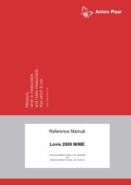
see Fig. 1. This has been interpreted as the sign that the 

landscape starts to ‘‘influence’’ the dynamical behavior 23. 

At T c , it is further argued, a second change in the landscape 

1063-651X/2003/684/04120113/$20.00 

68 041201-1 

©2003 The American Physical Society

L. BERTHIER AND J. P. GARRAHAN PHYSICAL REVIEW E 68, 041201 2003 

FIG. 1. Onset of slowing down in the binary Lennard-Jones 

mixture of Ref. 13. Three quantities are reported as a function of 

temperature T. i The logarithm of the relaxation time, log 10 in 

arbitrary units extending over four decades in time; a MCT powerlaw 

divergence, with T c 0.435, was used to fit this data in Ref. 

13. ii The energy of inherent structures, e IS , taken from Ref. 

43, which decreases markedly when the temperature decreases 

below T 0 1.0. iii The anharmonic part of Cartesian distance between 

configurations and their corresponding IS, (r) 2 

N 1 i (r i r (IS) i ) 2 aT, which displays a qualitative change 

around T c , taken from Ref. 23. 

properties takes place, which is indicated by several observations 

23–29. For example, the mean-square displacement 

from an equilibrated configuration to its corresponding inherent 

structure, N 1 i (r i r (IS) i ) 2 , is proportional to T below 

T c , as expected from pure vibrations in quadratic wells, but 

the temperature dependence changes above T c , revealing 

‘‘anharmonicities’’ in the landscape 23,24, see Fig. 1. 

Another indication of a topological change in the energy 

landscape was discussed in Ref. 30, in analogy with what 

happens in mean-field models 31,32: the vanishing as T 

approaches T c of the mean intensive number of negative 

directions intensive index of stationary points of the potential 

energy, n s (T). Numerical simulations 33–38 found that 

n s (T) decreases with decreasing T, and fits were performed 

to show that n s (T c )0 33–35. The physical interpretation 

of this result is the apparent existence at T c of a ‘‘geometric 

transition’’ between a ‘‘saddle dominated regime’’ above T c 

and a ‘‘minima dominated regime’’ below T c 39. T c would 

then really coincide with the appearance of activated processes, 

described in a topographic language as ‘‘hopping’’ 

between minima of the landscape. Analogous findings had 

been previously reported from instantaneous normal mode 

analysis of equilibrium configurations 40, also supporting a 

qualitative change in the landscape topology close to T c 

41,42. 

Figure 1 summarizes this MCT/landscape scenario with 

published numerical data 13,23,43 obtained for the standard 

supercooled liquid model of Ref. 13. 

B. Problems and contradictions 

At first sight Fig. 1 appears as convincing evidence in 

favor of the MCT/landscape interpretation of the dynamics. 

On closer inspection, however, the above scenario is less 

robust. Several qualitative and quantitative observations do 

not fit into the picture presented above. 

(i) Activated dynamics above T c . The main idea behind 

the landscape approach 20 is that vibrations and structural 

relaxations take place on very different time scales, so that 

the system is ‘‘trapped’’ and vibrates in one minimum before 

‘‘hopping’’ to another minimum. This is indeed observed using 

the mapping from trajectories to IS 21 in simulations of 

sufficiently small systems 44,45. We have also discussed 

theoretically this issue in a recent work 6. Given that numerical 

studies were performed much above T c , a crucial 

conclusion of Refs. 6,44,45 is that ‘‘activated dynamics’’ is 

indeed present in this temperature regime. 

(ii) Heterogeneous dynamics above T c . It is now well 

documented that the dynamics of supercooled liquids, even 

above the mode-coupling temperature T c , is heterogeneous 

in the sense that the local relaxation time has nontrivial spatial 

correlations 46. This phenomenon is not very different 

from what happens experimentally close to the glass transition 

T g 12. Besides, the decoupling between transport coefficients, 

which is also interpreted in terms of dynamical 

heterogeneity 12,47, is observed in numerical simulations 

above T c 13, although the effect is quantitatively less pronounced 

than in experiments near T g 48. 

(iii) Presence of saddles below T c . Despite claims based 

on numerical results that T c marks a real change in the topology 

of the landscape 33–35, there are strong indications 

that this is at best only a crossover 36,37, and at worst a 

biased interpretation of numerical data 38. For instance, 

careful numerical studies have shown that the saddle index 

n s (T) remains positive even below T c 36. Moreover, Ref. 

38 argues convincingly that the data for n s (T) can be described 

by an Arrhenius law, n s (T)exp(E/T), with E an 

energy scale, which means that T c does not mark any particular 

change in the saddle index. 

C. Alternative: real space physics and coarse-grained models 

The problems described above can be overcome through 

an alternative perspective on glass transition phenomena 

which puts the real space aspects of the dynamics at its core. 

This is the approach developed in Refs. 5–8. Interestingly, 

several of its central concepts, such as the relevance to the 

dynamics of localized excitations 49,50 and the importance 

of effective kinetic constraints 51,52, have been present in 

the literature for many years. Moreover, one of the original 

key observations of dynamic heterogeneity in glass formers 

was made by Harrowell and co-workers 53 in the models of 

Ref. 52. See Ref. 54 for an exhaustive review. 

Our approach relies on only two basic observations. 

i At low temperature mobility within a supercooled liquid 

is sparse and very few particles are mobile. This is somewhat 

equivalent to the statement that particles are ‘‘caged’’ 

for long period of times, as reflected by a plateau in the 

mean-square displacement of individual particles. 

ii When a microscopic region of space is mobile it influences 

the dynamics of neighboring regions, enabling them 

to become mobile, and thus allowing mobility to propagate 

in the system. This is the concept of dynamic facilitation 

041201-2

REAL SPACE ORIGIN OF TEMPERATURE CROSSOVERS ... 


50,52. The observation that very mobile particles in a supercooled 

liquid move along correlated ‘‘strings’’ 46 is a 

confirmation of this fundamental idea. 

From these two concepts it is possible to build effective 

microscopic models for glass formers by means of a coarsegraining 

procedure. This procedure can be schematically described 

as follows 7. Spatially, the particles are coarse 

grained over a length scale x of the order of the static 

correlation length given by the pair correlation function. This 

removes any static correlations between coarse-grained regions 

of linear size x. Cells are then identified according to 

their mobility by performing a coarse-graining on a microscopic 

time scale t. In its simplest version cells are identified 

by a scalar ‘‘mobility field,’’ n(r,t)0,1, the values 0/1 

corresponding to an immobile/mobile cell at position r and 

time t. The next step is to replace continuous space by a 

lattice, n(r,t)→n i (t). Mobile or excited cells carry a free 

energy cost, so when mobility is low it is reasonable to describe 

their static properties with a noninteracting Hamiltonian 

52, 

N 

H 

i1 

n i , 

1 

for a lattice of N sites. The link between mobility and potential 

energy 5 has also been observed in numerical simulations 

46. 

The coarse-graining procedure described above will generate 

local dynamical rules for the mobility field. The prominent 

feature of this dynamics will be dynamic facilitation, 

which in its simplest version states that a cell at site i is 

allowed to move only if it has an excited nearest neighbor 

52, 

C i c 

→ 

n i 0 

← 

n i 1, 

C i 1c 

where C i 1 j,i (1n j ), and j,i indicates nearest 

neighbor, and c represents the average concentration of excited 

cells easily deduced from Eq. 1, 

cTn i 1e 1/T 1 . 

Explicit examples where dynamic facilitation is generated 

under coarse graining can be found in Ref. 55. Clearly, 

different models are defined simply by changing the kinetic 

rules, e.g., the number or directionality of mobile neighbors 

required to move 54. Also, a more complex mobility field 

may be required to account quantitatively for all glass transition 

features 7. 

Crucially, we will show that the physical mechanisms 

which explain the onset of slowing down and crossovers 

between different dynamical regimes in supercooled liquids 

are generic to this class of models. This means that we can 

use the simplest of them, the Fredrickson-Andersen FA 

model defined by Eqs. 1 and 2 in one spatial dimension 

hereafter 1D FA model to make detailed predictions and 

calculations. 

2 

3 

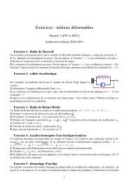
FIG. 2. Representative trajectories in the 1D FA model. The 

vertical axis is space, the horizontal one time. The three trajectories 

are for L150 and t2000. Excited cells or defects are black, 

unexcited ones white. The top frame is for T2.5, in the hightemperature 

regime where almost no isolated defects are present. 

The middle frame is for T1.0, the temperature regime where slow 

bubbles start to appear, seen here as large white domains. The bottom 

frame is for T0.5, where almost all defects are isolated. For 

T0.5, the mean relaxation time is 120, the mean dynamic correlation 

length 9, but it is clear that times and lengths are broadly 

distributed. 

II. PHYSICAL PICTURE OF DYNAMIC CROSSOVERS 

In order to understand the physics captured by the coarsegrained 

facilitated models defined above, it is useful to look 

at trajectories, that is, space-time representations of the dynamics 

5. We show in Fig. 2 three representative trajectories 

for the 1D FA model, where mobile cells defects are 

black, and immobile ones are white. From the trajectories, 

the principal observation is the appearance at low temperatures 

of nontrivial spatiotemporal correlations, seen as spatially 

and temporally extended domains of immobile cells 

delimited by isolated defects 5. In 1D they look like 

‘‘bubbles’’ 6, and trajectories are dense assemblies of these 

slow bubbles. This nanoscopic ordering in trajectory space is 

the cause of the phenomenon of dynamic heterogeneity observed 

experimentally and in simulations 5. Dynamic heterogeneity 

is the central aspect of the physics of supercooled 

liquids: it is naturally captured by our approach. 

The statistical mechanics of trajectories, rather than con- 



figurations, determines the dynamical behavior. For example, 

due to the noninteracting Hamiltonian 1, static correlations 

are trivial. However, when trajectories are considered, it is 

clear that cells become dynamically correlated. In other 

words, these models naturally predict the existence of a dynamical 

correlation (T) which grows when the dynamics 

slows down. This statement can be quantified 5,8,56,57 by 

studying multipoint functions, for example, C(i j,t) 

P i (t)P j (t)P i (t)P j (t), where P i (t) is a dynamical 

correlator at site i below we will consider the persistence of 

site i). The spatial decay of a function like C(i j,t) defines 

unambiguously the dynamical correlation length (T), 

as already discussed theoretically 5,8,56 and measured in 

numerical simulations 46,56–59. Furthermore, the joint 

distributions of time and length scales give rise to the canonical 

features of glass formers, such as stretched relaxation, 

decoupling between transport coefficients, and kinetic 

and thermodynamic strong and fragile behaviors 5–7. 

Let us take a closer look at the temperature evolution of 

the trajectories in Fig. 2. Starting from the very low temperatures 

where trajectories consist of a mixture of slow bubbles, 

the dynamics can be understood in terms of the opening and 

closing of bubbles, that is, the branching of an excitation line 

or the coalescence of two. As shown in Ref. 6, these events 

are the ‘‘hopping between minima’’ described in Ref. 20. 

Therefore, we have a clear understanding of ‘‘activated processes’’ 

and of their statistical properties 6. 

As temperature is increased, more and more defects are 

present. This has several consequences. First, the typical spatial 

and temporal extension of bubbles reduces, that is, the 

system becomes faster and less heterogeneous. Second, clusters 

of defects become more common. These objects are important 

because their dynamics is completely different from 

that of isolated defects. In a cluster, defects do not have to 

diffuse and create or annihilate other defects but can instantaneously 

relax in a much faster process. At high temperature, 

the dynamics is fast because almost no bubbles are 

present, and the dynamics is governed by clusters of defects. 

Interestingly, at some intermediate temperature middle 

frame in Fig. 2 a coexistence between clusters and isolated 

defects is observed, so that the dynamics has a ‘‘mixed’’ 

character. 

Clusters of defects disappear much faster with decreasing 

temperature than the overall concentration of defects. The 

probability to have a cluster of k defects is indeed p(k) 

c k , so that at low T we have p(1)p(2)•••. 

The coexistence of fast and slow processes with different 

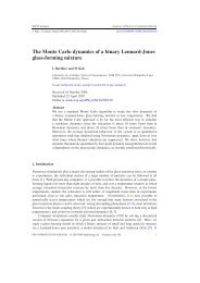
temperature behavior has a direct influence on the distribution 

of local relaxation times, which we present in Fig. 3 for 

various temperatures. At high temperature, T1.0, where 

fast processes are dominant, the distribution is exponential, 

with a mean which depends weakly on temperature below 

we discuss in detail its temperature dependence. Around T 

1.0, a shoulder develops in the large time tail of the distribution, 

corresponding to the appearance of the bubbles in 

the trajectories of Fig. 2. This marks the increasing relevance 

of slow processes and the growth of the dynamic correlation 

length beyond the microscopic high-temperature value. This 

FIG. 3. Distribution of the logarithm of the persistence time of 

individual cells, (ln) for various temperatures. T o 1.0 marks the 

appearance of a shoulder in the high-temperature distribution. For 

T c T0.6T o , two ‘‘processes’’ coexist. Fast processes disappear 

close to T c 0.3. 

temperature corresponds therefore to the onset temperature 

T o 1.0. 

Decreasing further the temperature, we clearly see a regime 

of mixed dynamics. At T0.6, for instance, there are 

two peaks in the distribution, reflecting the coexistence of 

clusters and isolated defects. At this temperature, the time 

scale has already increased by several orders of magnitude, 

and the dynamic correlation length is about (T0.6) 

c 1 (T0.6)6. 

Finally, further decrease in temperature makes clusters of 

defects very rare and we are left only with the contribution of 

isolated defects. This low-temperature distribution is the one 

discussed in Refs. 5,6, which in turn implies the stretched 

exponential decay of dynamical correlators. The contribution 

of clusters becomes negligible beyond a second crossover 

temperature, here T c 0.3. While this crossover temperature 

is not linked in any way to the mode-coupling singularity 

T c , this choice of notation will become clear shortly. 

From these distributions, it is possible to propose an empirical 

but quantitative determination of T o and T c . At each 

temperature T, the distribution is composed of fast processes 

(T), and slow processes (T), where (T) can 

be defined, e.g., as in Ref. 60. Requiring that slow processes 

are a significant fraction say 90% of the distribution 

leads to the definition of T c , 

 

 

(T c ) 

d0.9, 

where in an abuse of notation we also call () the distribution 

of persistence times. Requiring that slow processes, 

while not dominant in number, still contribute to a significant 

fraction of the mean relaxation time say again 90% leads to 

the definition of T o , 

 

 

(T o ) 

d0.9 . 

4 

5 




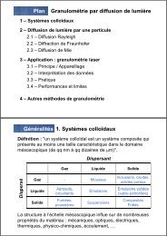
FIG. 4. Temperature regimes emerging from the discussion of 

Sec. II. T 0 marks the onset of slow dynamics, the appearance of the 

isolated defects bubbles, activated processes, and the growth of a 

dynamic correlation length. At T c , traces of the high-T physics 

clusters become negligible in the distributions of relaxation times. 

The crossover region T c TT o has therefore a mixed character. 

In Fig. 4, we summarize the physical picture that emerges 

from the considerations of this section. From the distributions 

of Fig. 3, we recognize that the dynamics becomes 

slow when the temperature is decreased below the onset temperature 

T o . This distinguishes the trivial liquid and the slow 

glassy regimes. From the trajectories of Fig. 2, we were also 

able to distinguish between fast, nonactivated processes 

clusters, and slow, activated processes isolated defects, 

bubbles. The former, typical of the liquid high-T physics, 

become negligible below T c , while the latter, typical of the 

low-T physics, appear at the onset temperature T o . As a 

consequence, the crossover region T c TT o contains 

traces of both high-T and low-T physics, as observed in the 

time distributions of Fig. 3. 

III. QUANTITATIVE CONSEQUENCES 

The physical picture we have presented for the onset of 

slowing down, based on the increasing relevance of a dynamically 

heterogeneous evolution of the system, leads to 

quantitative predictions which are in good agreement with 

previous numerical and experimental studies, as we discuss 

in this section. 

A. Dynamical correlators 

The basic dynamical quantities recorded in experiments 

and simulations of supercooled liquids are spatially averaged 

two-time functions. Simulations usually focus on the time 

domain and typically consider density-density correlation 

functions, while experimental results are often expressed in 

the frequency domain, measuring for instance dielectric susceptibilities. 

We will only consider systems in equilibrium so 

that the information content of both kinds of measurements 

is equivalent. 

From the distributions of times, Fig. 3, it is easy to derive 

dynamical correlators for the 1D FA model considered here. 

The spatially averaged persistence function reads 

041201-5 

FIG. 5. Persistence functions in the 1D FA model for the same 

set of temperatures as in Fig. 3. Symbols are numerical data and full 

lines are fits to the stretched exponential form expected theoretically 

for low temperatures, P(t)expt/(T) , with 1/2. 

The behavior of P(t) as a function of time for various tem- 

t 

Ptexp T , 

7 

 

Pt d. 6 

t 

peratures is shown in Fig. 5. At very low temperatures, the 

persistence function is known exactly due to the diffusion 

properties of isolated defects, and one gets 

where (T) is the relaxation time discussed in the following 

section. For the 1D FA model, 1/2, but the stretching 

exponent might be temperature dependent in more elaborated 

fragile models 6,54, as is indeed observed in experiments 

1,2. 

We see from Fig. 5 that for T0.2 and 0.3 P(t) is well 

approximated by Eq. 7 on the whole time window. For 

higher temperatures, TT c 0.3, the mixed character of the 

correlators is evident from the fact that Eq. 7 only describes 

the long time behavior of the correlator, as expected. In this 

temperature regime, short times are best described by a 

simple exponential. In the high-temperature regime, TT o 

1.0, relaxation is just exponential for all times. We conclude 

that the appearance of isolated defects at T o is reflected 

in the long-time behavior of dynamical correlators. In the 

crossover region, T c TT o , more and more of the decorrelation 

is due to isolated defects when T decreases. Below 

T c the entire decorrelation is due to these slow processes. 

A confirmation of the progressive domination of slow 

over fast processes described above can be found in the numerical 

results of Ref. 26. The similarity of Fig. 4 of Ref. 

26 and our Fig. 5 is in fact quite striking. In particular, Ref. 

26 calculated density-density correlations from both real 

configurations and their corresponding IS in a binary 

Lennard-Jones mixture. The latter, where thermal energies 

were removed in the quenching procedure, are the ones 

which have to be compared with Fig. 5, since fast vibrations 

are also removed in our coarse-grained approach. 

An important conclusion is that the long-time decay of 

dynamical correlators, sometimes referred to as the


diffusion with a temperature dependent diffusion constant, 

D(T)cexp(1/T). The system relaxes when defects 

have diffused over a distance given by the mean separation 

between defects, c 1 , so that 

ex TD 1 c 2 exp 3 T . 

9 

FIG. 6. Temperature dependence of the relaxation time in the 

1D FA model, (T). Open circles correspond to numerical data. 

Three fits are presented. The dashed line is the simple mean-field 

Hartree-like approximation, MF exp(1/T). The dotted-dashed line 

is the low-T exact behavior, ex exp(3/T). The full line is a powerlaw 

MCT-like fit, MCT (TT c ) with 2.3 and T c 0.3. The 

inset shows that the apparent power-law behavior is acceptable in a 

range of three decades in times. The main figure shows that low-T 

and high-T fits account for the whole temperature range. 

relaxation, is due to the presence of isolated defects and 

therefore of heterogeneous dynamics, even in the TT c regime. 

This means that activated dynamics, in the language of 

MCT, or hopping events in topographic terms, are responsible 

for the relaxation, even at temperatures well above 

T c . This conclusion is unavoidable in view of the numerical 

data of Refs. 26,44,45. 

B. Relaxation time 

The next natural quantity to consider, the relaxation time 

(T), is readily obtained from the dynamical correlators discussed 

in the preceding subsection. From the discussion of 

Sec. II, we expect a crossover from high-T to low-T at the 

onset temperature T o ; see Eq. 5. Our results for the 1D FA 

model are presented in Fig. 6, where (T) is defined as the 

time where the persistence function has decayed to the value 

1/e. 

The simplest mean-field approximation to the dynamics 

of the FA model consists in a Hartree-like decoupling of 

spatial correlations, n i n j →n i n j , in the dynamical equation 

for n i . This amounts to replacing the actual neighborhood 

of site i by an average neighborhood, and spins are 

always facilitated with an average rate equal to c. This gives 

a mean-field estimate of the relaxation time 61, 

MF Tc 1 exp 1 T . 

Figure 6 shows that this simple approximation accounts for 

the dependence of the relaxation time at high-temperatures, 

TT o . 

The exact result for the relaxation time of the 1D FA 

model is obtained by realizing that isolated defects undergo 

8 

This mechanism relies on the notion of dynamic facilitation 

which implies that local fluctuations of the mobility determine 

the dynamics, and is essentially beyond the reach of 

any mean-field type of approximation 53. We see from Fig. 

6 that Eq. 9 accounts for the behavior at low-temperatures, 

TT o . Figure 6 also presents a fit to the data with an MCT 

power-law form for the relaxation time 9, 

MCT TTT c , 

10 

similar to the one obtained in Ref. 52 for the two-spin 

facilitated, two-dimensional version of the FA model. 

From Fig. 6, we draw the following conclusions. The behavior 

of the relaxation time changes from the high-T to 

low-T behavior close to the onset temperature T o . The combination 

of simple mean field at high T with the exact form at 

low T allows to describe the temperature dependence of the 

relaxation time over the whole temperature range. However, 

given that (T) smoothly interpolates between these two different 

functional forms, the MCT power-law form, Eq. 10, 

appears to work reasonably well in a time window of about 

three decades see inset in Fig. 6. This range of apparent 

power-law behavior is in fact larger than the corresponding 

one in the canonical binary Lennard-Jones mixture of Ref. 

13, where extensive tests of MCT have been performed. 

Remarkably, we also find that the T c extracted from the 

power-law fit to the relaxation time coincides well with the 

temperature where fast processes cease to contribute in a 

significant manner to the distribution of relaxation times, 

Fig. 3. This explains our choice of notation for the lower 

crossover temperature T c . 

Following the standard MCT reading of the data 

10,11,13, we would erroneously conclude that activated 

processes only appear close to T c 0.3, since these processes 

are often tautologically defined by the breakdown of the 

power-law behavior of the relaxation time 11. Figures 3, 5, 

and 6 prove instead that activated dynamics starts to be relevant 

at T o , much above T c , dominating the relaxation of 

the correlators, and hence the relaxation time of the system. 

The results of this section considerably weaken the possibility 

of the existence of a temperature regime in supercooled 

liquids where the relaxation time is correctly described by a 

power-law behavior. It follows that the standard determination 

of the location of the MCT ‘‘singularity’’ T c in experiments 

and simulations is physically unjustified 62,63. In 

fact, the issue of the location of T c has been recently addressed 

in Ref. 64, where it was found that for a variety of 

systems, the temperature T c obtained from the actual MCT 

equations systematically coincides with the onset temperature 

T o discussed above. 



FIG. 7. Onset of the slowing down in the 1D FA model. We 

show three quantities as a function of temperature T. i Logarithm 

of the relaxation time, log 10 , see Fig. 6. ii Energy of IS, e IS , 

which displays a qualitative change around T o 1.0. iii Concentration 

d of cells moved in the descent from an equilibrium configuration 

to its IS, which displays a qualitative change around T c 

0.3. This figure should be compared with Fig. 1. 

C. Crossover temperatures 

Let us now consider the quantities shown in Fig. 1 as 

evidence in favor of the MCT/landscape picture in Lennard- 

Jones mixtures, from the perspective of dynamically facilitated 

models. In Fig. 7 we show for the 1D FA model a plot 

analogous to Fig. 1. 

The first quantity presented in Fig. 7 is the logarithm of 

the relaxation time, log 10 (T), as a function of temperature, 

which we discussed in detail in the preceding subsection. 

The second quantity shown in Fig. 7 is the average energy 

of inherent structures, e IS . For the 1D FA model it can be 

computed analytically by solving the zero-temperature dynamics 

of the model 65, 

e IS Tc e c , 

11 

where the concentration of defects, c, is defined in Eq. 3.At 

high-temperature e IS changes very slowly. When T is reduced 

below T o the concentration of defects starts to decrease 

markedly, and e IS follows the same trend, as can be 

seen in Fig. 7. This change in behavior at the onset temperature 

T o is due to the appearance of isolated defects, and 

therefore of a heterogeneous dynamics, and not to any special 

change of the potential energy surface. This is a very 

different interpretation of the physics from that of Ref. 23. 

The third quantity shown in Fig. 7 is analogous to the 

distance between a configuration and its nearest IS see Fig. 

1. In the lattice models we are considering the natural quantity 

to compute is the concentration of sites which change 

during the descent towards the inherent structure, d(T). 

Since only excited sites can change during this procedure, 

we get 

dTce IS c1e c . 

12 


Clearly, at low temperature dc 2 exp(2/T). This behavior 

is physically natural. Contributions to d(T) come from 

clusters of defects, which are the only objects that can relax 

during the descent to an IS. Since the probability for a cluster 

of k defects, p(k), goes as p(k)c k , the main nontrivial 

contribution to d(T) at low T comes from the smallest clusters, 

k2. These relax only one defect in the descent, so that 

dp(2)c 2 . Moreover, our defect interpretation is consistent 

with real space observations in simulations of silica 27, 

where it was found that during the descent to the IS the 

major contribution to the distance comes from annihilation 

of localized topological defects of the amorphous structure. 

The similarity of Fig. 7 to Fig. 1 is striking. The emerging 

physical picture, is however, completely different from the 

one of the MCT/landscape scenario. For example, while it 

may appear from the behavior of d(t) above T c that this 

quantity extrapolates to zero when T→T c see Fig. 7, the 

exact temperature dependence of d(T) is purely Arrhenius. 

This means that T c has no particular importance T c would 

not look special in a plot of d(T) versus 1/T]. Even if one 

accepts T c as delimiting two regimes with high and low concentrations 

of clusters of excitations, this apparent crossover 

is completely irrelevant as far as the long-time dynamics is 

concerned. These observations suggest that the crossover at 

T c from ‘‘landscape influenced’’ to ‘‘landscape dominated’’ 

of Ref. 23 is not physically significant for the relaxation. 

IV. INTERPRETATION OF ‘‘LANDSCAPE’’ PROPERTIES 

In recent years, the potential energy landscape of supercooled 

liquids has become an object of study per se 3. In 

Ref. 6, we have developed the idea that the main motivation 

behind these works was the observation of the separation 

between fast vibrations and slow hopping processes if 

sufficiently small systems are considered. This apparently 

harmless statement on the system size, we argued in Ref. 6, 

results in fact from the central feature of the dynamics of 

supercooled liquids: ‘‘sufficiently small’’ really means ‘‘if 

the system size is of the order of the dynamical correlation 

length (T)’’ 6,25. However, in a purely topographic description 

of the physics based on the statistical properties of 

minima, the relevance of the dynamical correlation length is 

not obvious 66. In that sense, a topographic description of 

the glass transition misses a central aspect of the physics. 

We shall show below that using the very simple spatial 

approach described in previous sections, we can trivially derive 

the statistical properties of the landscape reported in 

recent years. This successful confrontation to such an 

amount of apparently nontrivial and detailed numerical results 

is again a strong indication of the validity of our approach. 

A. Real space description of ‘‘minima’’ and ‘‘saddles’’ 

Reference 6 described in detail the connection between 

the nanoscopic ordering in the trajectories of dynamically 

facilitated models and the dynamics between IS, ‘‘metabasins,’’ 

or ‘‘traps’’ observed in numerical simulations or experiments 

of supercooled liquids. This same approach can be 



FIG. 8. Top: zoom on the low-T trajectory of Fig. 2. The vertical 

arrow indicates the closing of a bubble. Bottom left: expanded view 

of this event, showing two excitation lines meeting and coalescing. 

A cluster of three spins is needed for this process to occur. Bottom 

right: corresponding ‘‘reaction path.’’ Before the event there are two 

isolated defects energy 2), a cluster of three defects energy 

3) during the event, and one isolated defect after energy 1). 

extended to account for the properties of ‘‘saddles,’’ i.e., configurations 

related to transitions between IS. 

Figure 8 zooms on the lowest-temperature trajectory of 

Fig. 2. The top panel of Fig. 8 shows diffusion of isolated 

defects. It also shows coalescence and branching events, i.e., 

closing and opening of bubbles. These two kinds of processes 

correspond to ‘‘hopping’’ events between dynamical 

‘‘traps’’ 6. Let us consider in detail one of these events, for 

example, the coalescence process enlarged in the bottom left 

panel of Fig. 8. Isolated defects diffuse by first facilitating 

one of their neighbors, for instance, 

10→11→01. 

13 

For two defects to coalesce the minimum number of excitations 

that have to be present when they merge is three, 

101→111→011→010. 

14 

In this sequence, the total number of defects is 2 at the beginning, 

3 at the transition, and 1 at the end. This process is 

schematically described in the bottom right panel of Fig. 8. 

In topographic terms, an isolated defect corresponds to a 

local minimum of the energy, since such a configuration can 

only evolve by an energy increase, as in Eq. 13. Onthe 

other hand, a cluster of three excitations corresponds locally 

to a saddle point, since it is the transition configuration between 

two minima, as in Eq. 14 and Fig. 8. Larger clusters 

thus correspond to higher order saddles, since the larger the 

cluster the larger the number of possible moves into minima. 

The case k2 is particular: it is not a minimum since it can 

relax one defect to decrease its energy, but it is not a saddle 

either since it does not correspond to a hopping event like 

that of Fig. 8. Clusters with k2 are just ordinary points 

i.e., not stationary points of the landscape. The previous 

discussion generalizes in a natural way to the whole class of 

dynamic facilitated systems. 

FIG. 9. Saddle index versus energy difference between saddle 

and minima computed analytically for the 1D FA model for T 

0,) and p s 1/2. The obtained linear behavior is a natural consequence 

of i dynamic facilitation, ii localized defects, and iii 

dynamic heterogeneity. 

B. Absence of ‘‘geometric transition’’ 

The above identification between the relevant dynamical 

objects, isolated defects and clusters of defects, and ‘‘landscape 

properties’’ allows one to compute quantities such as 

the mean saddle index, n s (T), and the corresponding mean 

energy of stationary points, e s (T). 

The quantities n s and e s were estimated numerically in 

simulations of supercooled liquids 33,34. It was found that 

both functions decrease when T decreases, and extrapolations 

were performed that indicated n s (T c )0. Also, plotting the 

dependence of n s on e s e IS parametrized by the temperature, 

a simple linear relation was obtained, n s (e s e IS ) 

33–35. 

In the case of the 1D FA model, it is very simple to devise 

a procedure to go from an equilibrium configuration to the 

‘‘nearest’’ stationary point. Isolated defects and clusters of 

defects with k3 are locally such points, so we only have to 

deal with k2 clusters. From these we can either reach a 

‘‘minimum’’ k1 or a saddle with k3. We, respectively, 

assign the probabilities p s and (1p s ) to these two possibilities. 

We then have 

and 

 

n s T 

k1 

 

e s T 

k1 

pkn s k 

pke s k, 

15 

16 

where p(k)(1c) 2 c k is the probability to have a cluster of 

size k. From the discussion above we know that n s (1)0, 

e s (1)1, n s (2)(1p s ), e s (2)p s 3(1p s ), n s (k 

3)e s (k3)k. Putting all together we obtain 

n s T3c 21p s 1c c 2 1 2 3 

c 17 



and 

e s Tc12p s c 2 1c 2 . 

18 

At low T both quantities scale as n s c 2 and e s c. Three 

important conclusions can be drawn. 

i It is obvious from Eq. 17 that n s (T)0 for T0. 

This means that there is no ‘‘geometric transition’’ to a regime 

with vanishing saddle index. 

ii The saddle index has a temperature dependence which 

follows closely that of the distance d(T) discussed in the 

preceding subsection. This is expected because they both receive 

their principal contribution, at low T, from clusters 

with k2. In other words, the main objects for the lowtemperature 

dynamics, the isolated defects, do not contribute 

to these quantities. Therefore, as for the distance d(T) in Fig. 

7, the rapid decrease of n s (T) when the temperature decreases 

can easily be confused with a vanishing of the saddle 

index close to T c . 

iii The linear relation between n s and e s e IS becomes 

exact at low-temperatures, see Eqs. 11, 17, and 18. 

Again, the difference between e s and e IS comes from the 

clusters of defects which are relaxed during the descent to 

the inherent structure. In Fig. 9, we show the behavior of n s 

versus e s e IS for the entire range T0,). Note that in 

Ref. 33 a linear behavior between n s and e s was also reported. 

This is true at relatively high temperature, given that 

above T o the energy of inherent structure is almost constant 

while n s and e s change with temperature in the same way. 

These results are valid beyond the FA model which we 

have used to illustrate them. The inexistence of the geometric 

transition where the saddle index vanishes follows from the 

observation that the low-temperature behavior of n s is given 

by the smallest cluster of defects necessary to make a transition, 

in the sense described in the preceding section. Since 

these objects are spatially localized, their energy cost is 

O(1), and they exist with non zero probability at finite temperature 

T0. This argument is close in spirit to Stillinger’s 

argument for the inexistence of an entropy crisis at the Kauzmann 

temperature involving point defects 67. Moreover, as 

discussed in the Introduction, careful numerical simulations 

both confirm that n s (TT c )0 36,37, and report an 

Arrhenius behavior n s (T) 38, in agreement with our results. 

The relation between saddle index and energy, 

n s e s e IS , 

19 

which was first observed numerically 34,33,35, is also a 

general result for dynamically facilitated systems. This relation 

contains two different pieces of information. First, it 

shows that the intensive saddle index is a number of O(1). 

This is again a trivial consequence of the existence of the 

dynamical correlation length (T), so that a large sample 

can, in fact, be thought of an assembly of independent subsystems 

of linear size (T) 6. Second, and more interesting, 

is a connection between energy and saddle index, presented 

as a ‘‘general feature of the potential energy landscape 

of supercooled liquids’’ 35, for which no theoretical explanation 

was, however, available. This feature is, in fact, almost 

a tautology in the context of facilitated models: the 

more defects are present, the more available directions to 

move, the higher the energy above that of the IS. The fact 

that relation 19 holds in different model liquids is another 

confirmation that dynamical facilitation is a key generic feature 

of the dynamics of supercooled liquids. 

C. Thermodynamics and ‘‘anharmonicities’’ 

Another common procedure of the landscape approach is 

to decompose configurations into vibrational and configurational 

components. Stillinger and Weber 22 suggested to 

perform this decomposition at the level of the partition function, 

ZT 

EIS 


E IS exp E ISFT;E IS 

T 

, 20 

where the sum is over energies of IS, E IS , their number is 

indicated by (E IS ), and F(T,E IS ) is the ‘‘basin free energy’’ 

which takes into account fluctuations within an IS due 

to vibrations and possible ‘‘anharmonicities’’ i.e., all the 

rest. 

It is instructive to consider the calculation of the partition 

function in the case of the 1D FA model using the Stillinger 

and Weber decomposition. The thermodynamics of the FA 

model is that of a noninteracting gas of binary excitations. 

This simple thermodynamics, however, can be obtained with 

any dynamics obeying detailed balance with respect to 

Hamiltonian 1, the actual FA dynamics defined by Eq. 2 

being just one possibility. In this sense, the Stillinger and 

Weber prescription for thermodynamics is an approximation 

for the way a thermodynamic quantity would be calculated 

using a particular choice of dynamics to sample the configuration 

space. Inherent structures, basin free energies, etc., 

have no thermodynamic meaning, they only have a dynamical 

meaning associated with a particular choice of dynamics. 

For the 1D FA model we can evaluate the Stillinger and 

Weber partition function exactly. We have 

N/2 

NE 

Z N T 

EIS 

 

IS ! 

0 E IS !N2E IS 

 

! exp 1 T E IS 

F anh T;E IS . 

21 

The first factor counts the number of configurations of energy 

E IS with only isolated defects in a system of N sites. 

Due to the coarse-grained nature of facilitated models the 

only contribution to the basin free energy comes from anharmonicities. 

Performing the sum in Eq. 21 without the anharmonic 

contribution gives 



an IS all defects are isolated. The contribution of clusters of 

defects is obtained from the probability that an isolated defect 

in the IS was a cluster in the original configuration, 

which is given by Eq. 25. 

Interestingly, a numerical procedure to evaluate the anharmonic 

contributions can be proposed. First, the harmonic 

expression 23 is evaluated. Then, the approximate expression 

F anh T;E IS E IS Tf harm T 

26 

FIG. 10. Comparison of the various expressions for the free 

energy divided for convenience by T) in the 1D FA model: f ex is 

the exact free energy 24; f harm is the purely harmonic evaluation 

23 which is a good approximation below T c 0.3, and f 1 is the 

result obtained with expression 26 for anharmonicities which is 

good up to T o 1.0. 

Z N harm Texp N 2T U N i 2 exp 1 

2T, 

22 

where U N (x) is the Nth Chebyshev polynomial of second 

kind. In the thermodynamic limit the above expression simplifies 

to give the free energy in the ‘‘harmonic’’ approximation, 

f harm T lim T 

N→ 

N ln Z NT 

T ln2T ln114 e 1/T . 

23 

In Fig. 10, we compare approximation 23 to the exact 

expression for the free energy, 

f ex TT ln1e 1/T . 

24 

As observed numerically in supercooled liquids 3, both 

thermodynamic evaluations, Eqs. 23 and 24, apparently 

coincide below T c when anharmonicities become negligible. 

From the previous sections we know that anharmonicities are 

just a consequence of the existence of clusters of defects. At 

low-temperature the difference between Eqs. 23 and 24 is 

therefore proportional to c 2 , reflecting the fact that: i anharmonicities 

do not disappear below T c , which again is no 

particular temperature in this context; ii anharmonicities 

are due to clusters of defects, k2 being the leading term at 

low temperatures. 

In the particular case of the FA model we can formulate 

an exact expression for the anharmonic free energy F anh .It 

is easy to check that the choice 

F anh T;E IS E IS T f ex T 

25 

in Eq. 21 yields the exact expression for the free energy in 

the thermodynamic limit. This exact expression for the anharmonic 

part of the free energy is simple to understand. In 

can be used as an educated guess for the anharmonic contributions. 

This gives in turn a first order free energy f 1 (T). 

The improvement on the harmonic evaluation can be judged 

in Fig. 10, where we see that f 1 (T) coincides with the exact 

free energy up to TT o . This evaluation can then be improved 

iteratively using F anh (T;E IS )E IS (T) f 1 (T) to get 

f 2 (T), and so on. It is easy to show that, in our particular 

case, lim n→ f n (T) f ex (T). 

Although these results could lead to an improvement on 

present evaluations of anharmonic contributions in studies of 

the thermodynamics of supercooled liquids, they also show 

that topographic concepts are very far from the physical objects 

they pretend to describe. 

D. Failure of the Adams-Gibbs relation 

We end this section with a remark on the Adam-Gibbs 

relation, which is an attempt to connect dynamical properties 

to thermodynamic ones. The Adam-Gibbs formula relates the 

relaxation time of a glass former to the configurational 

entropy S c which would correspond to S c ln(E IS ) in the 

IS formalism: exp1/(TS c ). Apparently, this relation 

has been seen to hold both in numerical simulations and in 

experiments of various systems 3. A careful look at the 

published data reveals, however, that the correlation between 

relaxation time and entropy does not quantitatively satisfy 

the Adams-Gibbs relation. This important observation is often 

not clearly stated 3. 

Our analysis shows indeed that thermodynamic properties 

do not fully determine dynamical behaviors. Clearly, almost 

by definition, increases and S c decreases as temperature is 

lowered, but that is where the connection ends. It is easy to 

check that the Adam-Gibbs formula fails completely when 

applied to dynamic facilitated systems. We find instead that 

time scales are broadly distributed, the distribution of times 

being the result of an integral over a distribution of length 

scales, (), imposed by thermodynamic equilibrium, Eq. 

1. Crucially, however, dynamics also enters the integral in 

the form of the conditional probability of time and length, 

(t), which can be described, in a topographic language as 

containing information on the relevant ‘‘barriers,’’ which 

have a priori no obvious link with the statistics of minima. 

As a consequence, thermodynamics alone cannot be used to 

predict the dynamical behavior. Again, we find in the literature 

an excellent numerical confirmation of this statement. In 

Refs. 38,60, using a purely topographic description of a 

supercooled liquid, it was shown that the diffusion constant 



could be computed by a combination of thermodynamic and 

dynamical quantities, well in line with the above discussion. 

V. CONCLUSIONS 

In this paper, we have developed a spatial description of 

the physics of the progressive slowing down of supercooled 

liquids. The only ingredients in our method have been the 

notions of localized mobility excitations and facilitated dynamics 

5–8. Our results were illustrated explicitly for the 

simplest case of the 1D FA model, but are generic for this 

theoretical approach, and are in very good agreement with 

experimental and numerical observations in supercooled 

liquids. 

The physical picture which emerges from our work is, 

however, markedly different from that of the MCT/landscape 

scenario discussed in the Introduction. 

At high temperatures, TT o , the dynamics is fast and 

liquidlike, corresponding to the relaxation of large clusters of 

defects. Dynamic facilitation plays no major role, and a 

simple mean-field Hartree-like decoupling of the equations 

of motion yields predictions in good agreement with numerical 

results. 

When TT o , the dynamics becomes heterogeneous, in 

the sense that local relaxation times are spatially correlated 

in a nontrivial way. This can be seen in the trajectories of 

Fig. 2 as the appearance of slow bubbles 5,6. The long-time 

dynamics of the system results from the wide joint distribution 

of length scales and time scales, and the relaxation becomes 

stretched. This dynamic heterogeneity, which can be 

thought of as the activated dynamics invoked, but never described, 

by MCT, determines the relaxation and its temperature 

dependence for TT o . Also, dynamic heterogeneity 

implies that decoupling of transport coefficients actually 

starts at T o , as confirmed by the simulations. From a theoretical 

point of view, local fluctuations of mobility crucially 

influence the dynamical behavior. Any mean-field-like approach, 

no matter how involved, is most probably doomed to 

fail. 

At T o not all trace of high-T physics clusters of defects 

disappears. The dynamics has a mixed character in the range 

T c TT o , as seen, for example, in the behavior of dynamical 

correlators like in Fig. 5. The temperature T c is just a 

crossover. It is the temperature below which isolated defects 

not only dominate the long-time dynamics as for T c T 

T o ) but are also the most numerous dynamical objects, see 

Eq. 4. Clusters of defects, whose dynamics is homogeneous 

and nonactivated, are responsible for the temperature dependence 

of several quantities, such as distance between configurations 

and IS, saddle index n s (T), and anharmonic contributions 

to the free energy. In numerical simulations, T c has 

been interpreted as a key temperature, in accordance with 

MCT for which it represents a dynamical singularity. We 

have shown, however, that all of these quantities have a 

smooth temperature dependence, as has been recently observed 

numerically 36–38. This means that T c does not 

correspond to a transition or singular point, but is at most a 

crossover. Crucially, the objects which display a crossover 

close to T c are also irrelevant for the long-time dynamics, so 


that the inexistence of the singularity T c is anyway not a 

physically important issue for the relaxation. 

Below T c , isolated defects are the only remaining objects 

and the dynamics is dominated by the nanoscopic demixing 

of slow and fast regions so that trajectories look like a dense 

mixture of slow bubbles, which in turn gives a natural theoretical 

interpretation of the canonical features of glass transition 

phenomena 5–7. 

Our results, together with some other recent studies 

38,44,45,48,53,60,62–64,68, suggest that several essential 

features of the dynamics of supercooled liquids need to be 

recognized and we now list some of them. 

1 The dynamics is heterogeneous and activated well 

above T c . 

2 The dynamical slowing down of supercooled liquids is 

due to the growth, below T o , of a dynamic correlation length 

(T), or more precisely, of a whole distribution of length 

and time scales. 

3 The long-time dynamics, and therefore the relaxation 

time of the liquid is dominated by heterogeneous ‘‘activated’’ 

dynamics below T o . 

4 The MCT definition of activated processes as deviations 

from the ideal theory is incorrect. It is unlikely that the 

power-law behavior predicted by MCT correctly describes 

the temperature dependence of . The practical definition 

of the temperature T c cannot be used. 

5 No topological change of the potential energy landscape 

takes place close to T c . Quantities such as the saddle 

index and anharmonicities do not vanish close to T c and 

have a smooth temperature behavior. At best, they undergo a 

crossover from large to small which remains to be quantified. 

6 Even if one accepts T c as a crossover temperature, as 

in Eq. 4, quantities related to this crossover are unimportant 

for the long-time dynamics. 

7 Knowledge of thermodynamic properties is not 

enough to predict dynamical behavior, which explains the 

quantitative failure of relations like the Adams-Gibbs formula. 

The approach we developed in this paper, which is an 

extension of previous efforts 5–8, is generic. It can be applied 

both to systems like Lennard-Jones liquids or to hard 

sphere systems. It gives a perspective on the physics of glass 

formers which is clearly distinct to, and in many respects 

more natural than, that of MCT or topographic approaches. 

There are many important and interesting open questions 

which need to be addressed from this perspective. This include, 

among others, understanding properly the origin of 

mobility excitations, and the breakdown of Stokes-Einstein- 

Debye relations and associated decouplings between transport 

coefficients. 

A general conclusion that can be drawn from this work 

and our previous ones is that, in many respects, glass transition 

phenomenon is more standard than often assumed, in the 

sense that it is determined by the interplay between growing 

dynamic length scales and time scales. This is obviously 

reminiscent of critical phenomena 8, meaning that it should 

be possible to adapt renormalization group techniques to 

study the dynamics of the glass transition. 



ACKNOWLEDGMENTS 

We are grateful to J.-P. Bouchaud, G. Biroli, A. Buhot, A. 

Heuer, D.R. Reichman, G. Tarjus, and especially D. Chandler 

for useful discussions. We acknowledge financial support 

from CNRS France, Marie Curie Grant No. HPMF- 

CT-2002-01927 EU, EPSRC Grant No. GR/R83712/01, the 

Glasstone Fund, and Worcester College Oxford. Some of the 

numerical results were obtained on Oswell at the Oxford 

Supercomputing Center, Oxford University. 

1 M.D. Ediger, C.A. Angell, and S.R. Nagel, J. Phys. Chem. 100, 

13200 1996. 

2 C.A. Angell, Science 267, 1924 1995. 

3 P.G. Debenedetti and F.H. Stillinger, Nature London 410, 259 

2001. 

4 P. G. Debenedetti, Metastable Liquids Princeton University 

Press, Princeton, 1996. 

5 J.P. Garrahan and D. Chandler, Phys. Rev. Lett. 89, 035704 

2002. 

6 L. Berthier and J. P. Garrahan, J. Chem. Phys. 119, 4367 

2003. 

7 J.P. Garrahan and D. Chandler, Proc. Natl. Acad. Sci. U.S.A. 

100, 9710 2003. 

8 L. Berthier, Phys. Rev. Lett. 91, 055701 2003. 

9 W. Götze and L. Sjögren, Rep. Prog. Phys. 55, 551992. 

10 W. Götze, J. Phys.: Condens. Matter 11, A11999. 

11 W. Kob, in Slow Relaxations and Nonequilibrium Dynamics in 

Condensed Matter, edited by J.-L. Barrat, J. Dalibard, M.V. 

Feigel’man, and J. Kurchan, Springer-Verlag, Berlin, 2003, 

cond-mat/0212344. 

12 For reviews on dynamic heterogeneity, see, H. Sillescu, J. 

Non-Cryst. Solids 243, 811999; M.D. Ediger, Annu. Rev. 

Phys. Chem. 51, 992000. 

13 W. Kob and H.C. Andersen, Phys. Rev. Lett. 73, 1376 1994; 

Phys. Rev. E 51, 4626 1995; 52, 4134 1995. 

14 W. Götze and T. Voigtmann, Phys. Rev. E 61, 4133 2000. 

15 G. Tarjus and D. Kivelson, in Jamming and Rheology, edited 

by A. J. Liu and S. R. Nagel Taylor & Francis, New York, 

2001. 

16 E. J. Donth, The Glass Transition Springer-Verlag, Berlin, 

2001. 

17 E. Rössler and A.P. Sokolov, Chem. Geol. 128, 143 1996. 

18 F. Stickel, E.W. Fischer, and R. Richert, J. Chem. Phys. 104, 

2043 1996. 

19 C.A. Angell, J. Phys. Chem. Solids 49, 863 1988; J. Phys.: 

Condens. Matter 12, 6463 2000. 

20 M. Goldstein, J. Chem. Phys. 51, 3728 1969. 

21 F.H. Stillinger and T.A. Weber, Phys. Rev. A 25, 978 1982; 

28, 2408 1983; Science 225, 983 1984. 

22 F.H. Stillinger, Science 267, 1935 1995. 

23 S. Sastry, P.G. Debenedetti, and F.H. Stillinger, Nature London 

393, 554 1998. 

24 S. Büchner and A. Heuer, Phys. Rev. E 60, 6518 1999. 

25 S. Büchner and A. Heuer, Phys. Rev. Lett. 84, 2168 2000. 

26 T.B. Schroder, S. Sastry, J.C. Dyre, and S.C. Glotzer, J. Chem. 

Phys. 112, 9834 2000. 

27 P. Jund and R. Jullien, Phys. Rev. Lett. 83, 2210 1999. 

28 T. Keyes and J. Chowdhary, Phys. Rev. E 65, 041106 2002. 

29 For extension of the landscape ideas in the glass phase see: 

C.A. Angell, Y. Yue, L.M. Wang, J.R.D. Copley, S. Borick, and 

S. Mossa, J. Phys. C 15, S1051 2003; T.S. Grigera, V. 

Martin-Mayor, G. Parisi, and P. Verrocchio, Nature London 

422, 289 2003; for alternative real space interpretations, see, 

e.g., E. Duval, L. Saviot, L. David, S. Etienne, and J. F. Jal, 

Europhys. Lett. 63, 778 2003. 

30 A. Cavagna, Europhys. Lett. 53, 490 2001. 

31 J. Kurchan and L. Laloux, J. Phys. A 29, 1929 1996. 

32 A. Cavagna, J.P. Garrahan, and I. Giardina, Phys. Rev. B 61, 

3960 2000. 

33 K. Broderix, K.K. Bhattacharya, A. Cavagna, A. Zippelius, and 

I. Giardina, Phys. Rev. Lett. 85, 5360 2000. 

34 L. Angelani, R. Di Leonardo, G. Ruocco, A. Scala, and F. 

Sciortino, Phys. Rev. Lett. 85, 5356 2000. 

35 P. Shah and C. Chakravarty, J. Chem. Phys. 115, 8784 2001; 

T.S. Grigera, A. Cavagna, I. Giardina, and G. Parisi, Phys. Rev. 

Lett. 88, 055502 2002; L. Angelani, R. Di Leonardo, G. 

Ruocco, A. Scala, and F. Sciortino, J. Chem. Phys. 116, 10297 

2002; L. Angelani, G. Ruocco, M. Sampoli, and F. Sciortino, 

J. Chem. Phys. 119, 2120 2003. 

36 J.P.K. Doye and D.J. Wales, J. Chem. Phys. 116, 3777 2002. 

37 G. Fabricius and D.A. Stariolo, Phys. Rev. E 66, 031501 

2002. 

38 B. Doliwa and A. Heuer, Phys. Rev. E 67, 031506 2003. 

39 A. Cavagna, I. Giardina, and G. Parisi, J. Phys. A 34, 5317 

2001. 

40 S.D. Bembenek and B.B. Laird, Phys. Rev. Lett. 74, 936 

1995; J. Chem. Phys. 104, 5199 1996. 

41 C. Donati, F. Sciortino, and P. Tartaglia, Phys. Rev. Lett. 85, 

1464 2000; E. La Nave, H.E. Stanley, and F. Sciortino, ibid. 

88, 035501 2002. 

42 T. Keyes, J. Phys. Chem. 101, 2921 1997. 

43 W. Kob, J.-L. Barrat, F. Sciortino, and P. Tartaglia, J. Phys. C 

12, 6385 2000. 

44 B. Doliwa and A. Heuer, Phys. Rev. E 67, 030501 2003. 

45 R.A. Denny, D.R. Reichman, and J.-P. Bouchaud, Phys. Rev. 

Lett. 90, 025503 2003. 

46 See for a review, S.C. Glotzer, J. Non-Cryst. Solids 274, 342 

2000. 

47 G. Tarjus and D. Kivelson, J. Chem. Phys. 103, 3071 1995. 

48 P. Viot, G. Tarjus, and D. Kivelson, J. Chem. Phys. 112, 10 368 

2000; D.N. Perera and P. Harrowell, Phys. Rev. E 54, 1652 

1996. 

49 S.H. Glarum, J. Chem. Phys. 33, 639 1960; M.C. Phillips, 

A.J. Barlow, and J. Lamb, Proc. R. Soc. London, Ser. A 329, 

193 1972. 

50 P. W. Anderson, in Ill-Condensed Matter, edited by R. Balian 

et al. North-Holland, Amsterdam, 1979. 

51 R. G Palmer, D.L. Stein, E. Abrahams, and P.W. Anderson, 

Phys. Rev. Lett. 53, 958 1984. 

52 G.H. Fredrickson and H.C. Andersen, Phys. Rev. Lett. 53, 



1244 1984; J. Chem. Phys. 83, 5822 1985. 

53 S. Butler and P. Harrowell, J. Chem. Phys. 95, 4454 1991; 

95, 4466 1991; P. Harrowell, Phys. Rev. E 48, 4359 1993; 

M. Foley and P. Harrowell, J. Chem. Phys. 98, 5069 1993. 

54 F. Ritort and P. Sollich, Adv. Phys. 52, 219 2003. 

55 J.P. Garrahan and M.E.J. Newman, Phys. Rev. E 62, 7670 

2000; J.P. Garrahan, J. Phys. C 14, 1571 2002. 

56 S. Franz, C. Donati, G. Parisi, and S.C. Glotzer, Philos. Mag. 

B 79, 1827 1999; S.C. Glotzer, V. Novikov, and T.B. Schroder, 

J. Chem. Phys. 112, 509 2000. 

57 B. Doliwa and A. Heuer, Phys. Rev. E 61, 6898 2000. 

58 M.M. Hurley and P. Harrowell, Phys. Rev. E 52, 1694 1995; 

D.N. Perera and P. Harrowell, J. Chem. Phys. 111, 5441 

1999. 

59 Y. Hiwatari and T. Muranaka, J. Non-Cryst. Solids 235-237, 19 


1998. 

60 B. Doliwa and A. Heuer, e-print cond-mat/0306343. 

61 M. Schulz and S. Trimper, Phys. Rev. E 57, 6398 1998. 

62 X.C. Zeng, D. Kivelson, and G. Tarjus, Phys. Rev. E 50, 1711 

1994. 

63 X.C. Zeng, D. Kivelson, and G. Tarjus, Phys. Rev. Lett. 72, 

1772 1994. 

64 Y. Brumer and D.R. Reichman, e-print cond-mat/0306580. 

65 A. Crisanti, F. Ritort, A. Rocco, and M. Sellitto, J. Chem. 

Phys. 113, 10 615 2000. 

66 D. Kivelson and G. Tarjus, J. Phys. Chem. B 105, 11854 

2001. 

67 F.H. Stillinger, J. Chem. Phys. 88, 7818 1988. 

68 D. Kivelson, S.A. Kivelson, X. Zhao, Z. Nussinov, and G. 

Tarjus, Physica A 219, 271995.

Phys. Rev. E 68, 041201 - APS Link Manager - American Physical ...

You also want an ePaper? Increase the reach of your titles

Delete template?

Save as template?