Time Constant- Series RC Circuit with DC Applied

West Virginia University
College of Engineering & Mineral Resources
Objectives:
Lane Department of Computer Science and Electrical Engineering
Spring 2007
EE 224 Electrical Circuits Laboratory ESB – E 851
Experiment No.1
Time Constants-Series RC Circuit with DC Applied
For the student to measure current changes in a resistive-capacitive series circuit, then
using the measured current to determine resistor and capacitor voltages, next to plot these
changes on linear graph paper, and last to verify the experimental results by calculation.
Equipment Required
• Meters: Milliammeter
• Power Supply: DC power supply
• Resistor: 1 MΩ
• Capacitor: 10 µF, 50 V DC (electrolytic)
THEORY:
RC time constant circuits are used extensively in electronics for timing (setting
oscillator frequencies, adjusting delays, blinking lights, etc.). It is necessary to
understand how RC circuits behave in order to analyze and design timing circuits.
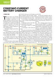
In the circuit below with the switch open, the capacitor is initially uncharged, and so
has a voltage, vc, equal to 0 volts. When the single-pole single-throw (SPST) switch is
closed, current begins to flow, and the capacitor begins to accumulate stored charge.
Since Q=CV, as stored charge (Q) increases, so too does the capacitor voltage (vc)
increase. However, the growth of capacitor voltage is not linear; in fact, it’s called an
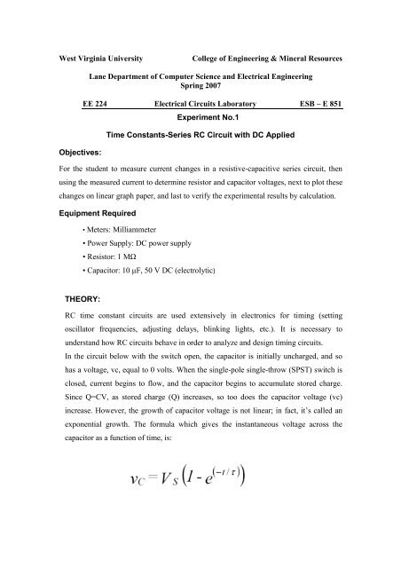
exponential growth. The formula which gives the instantaneous voltage across the
capacitor as a function of time, is:

This formula describes exponential growth, in which the capacitor voltage is initially 0
volts, and grows to a value of V S
after enough time has gone by. It is important to
understand each term in this formula in order to be able to use it as a tool.
The use of the above formula in any RC circuit is only possible if the symbols in the
equation are fully understood. The following definitions describe each of these
symbols:
V S
= The maximum possible voltage change that will occur in the circuit during a time
lapse of five time constants. For the voltage versus time graph shown below, V S
is 100
volts..
t = The elapsed time in seconds that the circuit voltages and currents have been
changing. For the voltage versus time graph shown below, t is in seconds.
τ = The time constant of the circuit, and the symbol is the lower-case Greek letter
TAU. τ is the product of R and C (τ = RC) in ohms and farads, and the unit of τ is
seconds. R is the total resistance in series with the capacitor, and C is the total
capacitance of the circuit.
v C
= The capacitor voltage at any instant of time after the switch closes.
e = The base of natural logarithms, a constant which equals about 2.7183.
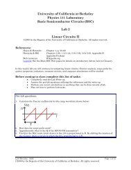
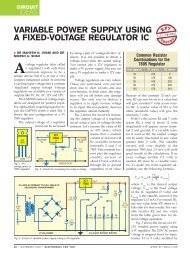
Figure 1 below is a graph of the capacitor voltage in a circuit where the time constant,
τ, is 1.0 second, and V S
is 100 volts. Notice that after about 5 seconds (i.e. 5 τ) the
capacitor voltage has grown from 0 volts to 100 volts, and the capacitor voltage is 100
volts and appears to have stopped changing. This is a condition called “steady-state”.
While in theory it takes an infinite time for “steady-state” conditions to be reached, in
practical terms, after five time constants using practical lab instruments it is nearly
impossible to measure any changes occurring.

Graph of capacitor voltage (vc) versus time
Procedure:
1. Construct the circuit shown below. Let R = 1 MΩ, 0.25 W, C = 10 µF (50 V
electrolytic), V S
= 20 V DC, and use an alligator lead jumper as the short circuit across
the capacitor.
2. Record the initial current reading of the milliammeter; it should be closed to “fullscale”
for a digital meter on the µA range (I = 20 V/1MΩ). Express the current in units
of µA.
Initial current = ____________µA
Write the above initial current value in the table on page 6, in the row for t = 0.0
seconds, for both Trial One and Trial Two.
3. Since it takes five times constants for a capacitor to fully charge, calculate one time
constant and five time constants for this circuit; if necessary, change your data table to
ensure that data is taken for no less than five time constants.

RC = 1τ
5(RC) = 5τ
Now get ready for some serious sustained data taking! This is best done with a partner,
but can be done successfully by one person. You will need a watch, (preferably a
stopwatch), or an analog wall clock with a second hand. The instant you remove the
alligator jumper, the current (which had been flowing through the jumper) flows
through the capacitor. This is time = 0, and you will begin recording data every 5
seconds after that instant.
4. Every 5 seconds, record the current under the Trial One column, until that column is
filled, on the data table on page 5 of this experiment.
5. Now repeat steps 3 and 4, because obtaining accurate, repeatable readings when the
current is changing is difficult. The results of Trial One and Trial Two will then be
averaged. Be sure to replace the alligator jumper before starting Trial Two. There
will be a significant spark the moment you put the jumper across the capacitor,
resulting from the rapid discharge of the energy stored in the capacitor, which brings its
voltage back to 0 volts.
6. Average the currents (Trial One and Trial Two) for each row in the data table, and
enter that average current in the table.
7. At each time in the table, using the average current at that time, calculate the resistor
voltage, using V R
= I(R); this is Ohm’s Law. Be sure to used the measured value of R.
8. Now, for each time in the table, using the calculated resistor voltage, calculate the
capacitor voltage using V C
= (V S
- V R
). Be sure to used the measured value of R. This is
just Kirchhoff’s Voltage Law applied: the sum of the resistor voltage and the capacitor
voltage must equal the source voltage.
9. It’s plotting time! Now you are going to construct a single graph, with two curves
(dependent variables) on it. You will plot v R
vs. time, and v C
vs. time. In setting up the
axes of your graph, note that the time axis should be in seconds. Also, realize that:
• The resistor voltage starts at V S
and exponentially decays to nearly 0 volts.
• The capacitor voltage starts at 0 volts and exponentially grows to nearly V S
volts.

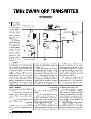
When your graph is done, it should look something like the following graph made with
Micosoft Excel.
Notice that Vc starts at 0 volts, and rises exponentially to 30 volts (the supply voltage). Vr
begins at 30 volts, and exponentially decays to 0 volts.

TIME
CURRENT
TRIAL 1 TRIAL 2 AVERAGE
RESISTOR
VOLTAGE
Vr
CAPACITOR
VOLATGE
Vc