Linear Circuits II

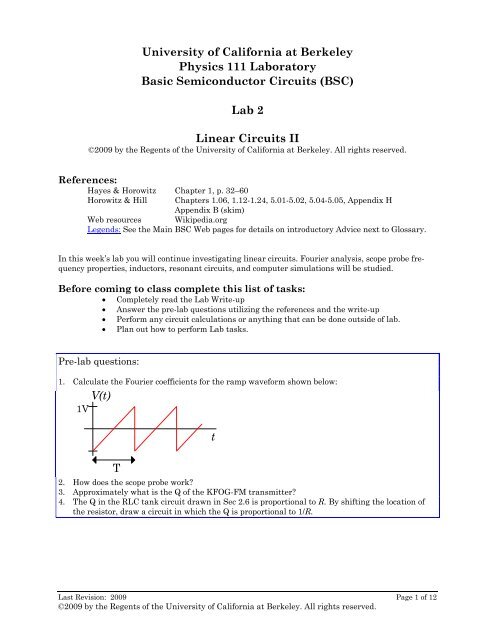
University of California at BerkeleyPhysics 111 LaboratoryBasic Semiconductor Circuits (BSC)Lab 2Linear Circuits II©2009 by the Regents of the University of California at Berkeley. All rights reserved.References:Hayes & Horowitz Chapter 1, p. 32–60Horowitz & Hill Chapters 1.06, 1.12-1.24, 5.01-5.02, 5.04-5.05, Appendix HAppendix B (skim)Web resources Wikipedia.orgLegends: See the Main BSC Web pages for details on introductory Advice next to Glossary.In this week’s lab you will continue investigating linear circuits. Fourier analysis, scope probe frequencyproperties, inductors, resonant circuits, and computer simulations will be studied.Before coming to class complete this list of tasks:• Completely read the Lab Write-up• Answer the pre-lab questions utilizing the references and the write-up• Perform any circuit calculations or anything that can be done outside of lab.• Plan out how to perform Lab tasks.Pre-lab questions:1. Calculate the Fourier coefficients for the ramp waveform shown below:1VV(t)tT2. How does the scope probe work?3. Approximately what is the Q of the KFOG-FM transmitter?4. The Q in the RLC tank circuit drawn in Sec 2.6 is proportional to R. By shifting the location ofthe resistor, draw a circuit in which the Q is proportional to 1/R.Last Revision: 2009 Page 1 of 12©2009 by the Regents of the University of California at Berkeley. All rights reserved.

Physics 111 BSC LaboratoryLab 2 Linear Circuits IITime Dependent CircuitsCircuit analysis is straightforward if all the signals are time independent, i.e. DC. The response ofcircuit to time dependent (AC) signals like sine waves is more complicated because the response tothe signal may not be in phase with the signal, and may depend on frequency. For example, a circuitdriven by a voltage source V = V 1 cos( ω t)might produce an output current phase-shifted by φ ,namely I = I 1 cos( ωt+φ ) . We can incorporate such phase shifts into Ohm’s law by allowing the voltages,currents, and resistances to be complex. Thus, I1 cos( ωt+ φ)becomes 1 Iexp( jωt ) , whereI = I 1 exp( jφ). While we do all our algebra with complex quantities, we have to take the real part inthe end (e.g. I = Re[ Iexp( jω t)] ) because we can measure only real quantities in the lab.Since I and V are not necessarily in phase, the resistance can no longer be a pure real quantity.We use a new term for complex resistances: the impedance Z. The magnitude of the impedance hasmuch the same function in Ohm’s law (now V = ZI ), as did the resistance R; it determines the relationbetween the magnitudes of I and V. The phase angle of Z determines the phase shift between Iand V. Note that resistance is redefined to be the real part of the impedance, and the reactance isdefined to be the imaginary part of the impedance.Clearly, a resistor has pure real impedance Z R= R and induces no phase shifts. Capacitors haveimpedance ZC =1 jωCand inductors have impedance ZL= jω L.Capacitor impedance decreases with frequency; inductor impedance increases with frequency. Bothcapacitors and inductors induce 90° phase shifts, but the phase shifts are in opposite directions.Any linear circuit 2 can be analyzed using the impedance formulas. The familiar parallel and seriesresistor addition formulas carry over directly; just substitute the capacitative and inductive impedancesfor R. For example, the impedance of two capacitors in parallel is1 1ZC1ZC2jωCj CZ ==1ω2 11=Z + Z + 1j C C( + )C1 C2 jωC1jωCω21 2Analyze any circuit just as you would if all the components were resistors, but keep track of thecomplex parts, and you will get the right answer. Thévenin circuit reduction works as well, thoughthe Thévenin resistance becomes a complex, frequency dependent impedance.And that’s all we need to know about complex impedances for this class. But as physicists we shouldunderstand the formal differential equations methods that underlie these simplifications, which canbe found in most E&M texts..BackgroundFourier Analysis and Repetitive WaveformsIn last week’s lab, we showed how the concept of complex impedances extends our ability to analyzecircuits to those driven by pure sinusoidal waveforms. However, our circuits will be frequently drivenby waveforms more complicated than pure sinusoids. Fortunately complex impedance analysis iseasily extended to include circuits driven by any repetitive waveform by using the fact that anyrepetitive waveform can be decomposed into a (possibly) infinite series of harmonic sinusoids. The1 To avoid confusion with the symbol for current, we use j instead of i for the −1 .2 More specifically, any circuit that consists only of resistors, capacitors, inductors, voltage sources,and current sources.Last Revision: 2009 Page 2 of 12©2009 by the Regents of the University of California. All rights reserved.

Physics 111 BSC LaboratoryLab 2 Linear Circuits IImathematical technique, which performs the decomposition, is called Fourier Analysis – you shouldhave already studied this technique in your mathematics classes. In summary, any waveform F(t)which is repetitive [has a period T defined such that F(t+T) = F(t) for all t] can be synthesized fromthe infinite sum∞( ) n ( )Ft () = ∑ Ansinnωt+B cosnωtn=0where the Fourier coefficients are defined asABBnn02=T2=T1=TT∫0T∫0T∫0( ω )Ft ()sinn tdt( ω )Ft ()cosn tdtFtdt () ,where ω = 2πT . The lowest order sinusoid (n=1) in the infinitesum is called the fundamental; all the other waveformsare referred to as the nth harmonic.For example, the square wave shown to the right has Fouriercoefficients An = 4 nπ for n odd, with all other coefficientsequal to zero.The beauty of using Fourier Analysis in circuit analysis is thatthe response of any linear circuit to a repetitive waveform is the sum of the responses of the circuit toeach individual harmonic. Thus a circuit with a transfer function H(ω), driven by the repetitivewaveform F(t), has an output1[ A sin( nωt) + B cos( nωt)]∑ ∞ no noH )n=0−4 10 5 s low pass filter [transfer function H ω( nωo.For example, when a 1kHz square wave is passed through aτ = ×( ) = 1 ( 1 + jωτ)],the calculation is summarized in the table below and the outputwaveform is shown in the graph to the right.Harmonic Frequency (Hz) Square WaveCoefficientLow Pass FilterTransfer Function111Output Coefficientsn ωnH ( ) A H n( ) A ( ω )2πA ω ωnn1 1000 1.273 0.941 – 0.236j 1.198 – 0.301j 1.2353 3000 0.424 0.638 – 0.481j 0.271 – 0.204j 0.3395 5000 0.255 0.388 – 0.487j 0.099 – 0.124j 0.1597 7000 0.182 0.244 – 0.43j 0.044 – 0.078j 0.0909 9000 0.141 0.163 – 0.37j 0.023 – 0.052j 0.05711 11000 0.116 0.116 – 0.32j 0.013 – 0.037j 0.03913 13000 0.098 0.086 – 0.28j 0.008 – 0.027j 0.02915 15000 0.085 0.066 – 0.248j 0.006 – 0.021j 0.022nnn H1ms1msLast Revision: 2009 Page 3 of 12©2009 by the Regents of the University of California. All rights reserved.

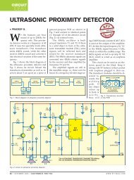
Physics 111 BSC LaboratoryLab 2 Linear Circuits IIResonant CircuitsA circuit combining an inductor and capacitor in parallel, sometimes called a1tank circuit, will oscillate at the frequency ω =LC .Such resonant circuits are frequently used in physics and electronics. Theyhave two primary applications: detecting signals oscillating at a known frequency,and generating signals at a specific frequency. The first application isexemplified by radio tuners which pick out a specific radio station (say atFigure 1 1MHz) from the enormous selection of available radio stations, and the secondis exemplified by the radio station transmitter itself, which must broadcastat a precisely controlled frequency. 3Resonant circuits are endlessly analyzed in the course textbooks. Here we will review only a fewpoints:• Understand the energy flow: the energy sloshes back and forth (at the resonant frequency) betweenthe capacitor (maximum capacitor voltage, no current) and the inductor (maximum current,no voltage across the capacitor.)• The oscillation amplitude of a resonant circuit will be much higher when driven with a frequencynear resonance than when driven off resonance. Thus, resonators will preferentially respond tonear resonant signals, and can be used to detect such signals even when these signals aremasked by signals at other frequencies.• Remember that the impedance of an inductor is proportional to j while the impedance of a capacitoris proportional to 1/ j = – j. Both inductors and capacitors induce 90° phase shifts, but inopposite directions. Consequently, their phase shifts are 180° apart from each other. At resonancethe magnitudes of the impedances are equal. Add them together and you get zero! Thusthe impedance of a series combinationof inductors and capacitors is zero,and the impedance of a parallel combination, like that drawn in Fig 1, is infinite.• Resonating circuits always have some dissipation, either from a deliberately added resistor orfrom imperfections in the circuit components. 4 The Q of a resonator is a measure of the “quality”of the resonator; the lower the dissipation, the higher the Q. There are several definitions of theQ:♦ 2π times the number of times the resonator will ring or oscillate after it has been hit with animpulse excitation before the voltage drops to 1/e.♦♦4π times the energy stored in the oscillator divided by the energy dissipated in one cycle.For a driven resonator, the oscillator resonant frequency ω divided by the detuning frequencyΔω. The detuning frequency is the driving frequency shift that results in the resonator poweramplitude dropping by a factor of two.♦ Approximately proportional to the amount that the oscillation amplitude peaks up whendriven at resonance compared to the amplitude when driven far off resonance.♦ Depending on the circuit configuration, various combinations of R, L, and C. Be warned…theQ is sometimes proportional to R, and sometimes to 1/R.These definitions work best for high Q.• A common misconception is that the highest possible Q is always best. Very high Q’s are desirablefor sources like transmitters, where very pure frequencies are needed. However, high Q’sare not necessarily desirable for receivers like radio tuners, which must detect a frequencyband 5 Δω. In such applications the resonator is designed so that its Q is approximately equal toω/Δω.3 For instance, KFOG-FM’s carrier frequency is allowed to drift only 2kHz (0.002%) from its assignedfrequency of 104.5MHz.4 Typical imperfections include resistance in the inductor windings and dissipation in the capacitordielectric.5 Radio stations need to transmit information, and information cannot be conveyed by a pure, singlefrequency wave. (The base, central frequency is called the carrier frequency.) Consequently stationsLast Revision: 2009 Page 4 of 12©2009 by the Regents of the University of California. All rights reserved.

Physics 111 BSC LaboratoryLab 2 Linear Circuits IISimulationsNumeric computer simulations have revolutionized many fields of physics and electronic design.Today’s astonishingly powerful desktop computers have made simulations a common tool of almostevery physicist. Simulations are used in every field: in condensed matter physics, astrophysics,plasma physics, even biophysics. And modern integrated circuits are almost entirely designed withthe aid of computer tools and simulations. BUT beware of the allure of simulations. While simulationshave their place for analytically intractable problems, an analytic solution is almost alwaysworth a thousand computer simulations. Use them for problems like the band structure of a complicatedcrystal or to find the attractors in a chaotic system. Don’t use them to solve for the behavior ofa simple harmonic oscillator.That said, in this course you will use computer simulations to study circuits that are, by and large,analytically tractable. Worse yet, all the circuits will be readily constructible on a breadboard.Always trust an experimental result over an analytic result 6 , and trust an analytic result over asimulation. So why are we having you run simulations? Our primary purpose is for you to get aflavor of what computer simulations can do, and how they can be run. In addition, some phenomenalike phase shift scaling can be studied more easily with the simulations than in the lab.You will be required to simulate a small number of circuits as part of this course. If simulatingstimulates you, you can play with many other circuits on your own. The circuits indicatedby the computer icon are available in the lab and over the web. You can also design andsimulate your own circuits.The circuit simulator we use is called PSpice, and is written by MicroSim Corporation. PSpice isbased on Spice, a very powerful circuit simulation engine which was developed here at Berkeley.Spice by itself is almost impossible to use; it requires input in an obscure format reminiscent of thecomputer input cards that went out in the 70s. Many commercial companies have incorporated theSpice engine into commercial products. PSpice is one such implementation. It has a decent MSWindows front end that mostly hides the native Spice input format, and an adequate back endgraphing program that displays the results of your simulations. A slightly reduced version of theprogram is available free, and can be downloaded from the web.PSpice works by solving the system of differential equations, which corresponds to the entered circuit.It automatically selects the low level differential equations appropriate for each circuit componentfrom a library of models, and then, according to the circuit topology, joins these low level differentialequations into one master system of differential equations. Finally it solves this systemnumerically and graphs the results. For example, for the RC high-pass filter below, the capacitor ismodeled by the differential equation dVC/dt = I/C, and the resistor by the trivial differential equationVR = RI. 7 The computer then automatically constructs and solves the system differential equation,dV/dt = RdI/dt + I/C.The solution can be graphed as a function of time. Such solutions are called transient analyses.Perhaps more useful is PSpice’s ability to scan the master differential equation over a set of frequen-broadcast radio waves in a band surrounding their carrier frequency. For example, the stationKFOG-FM’s carrier frequency is at 104.5MHz, but it actually broadcasts between about 104.450 and104.550MHz.6 To be fair to the theorists, remember that this statement was written by an experimentalist.Experimental results are sometimes wrong: witness Cold Fusion.7 An active circuit element, such as a transistor, requires a much more complicated model. Fortunately,tens of thousands of such models are available in the libraries that come with the program.Last Revision: 2009 Page 5 of 12©2009 by the Regents of the University of California. All rights reserved.

Physics 111 BSC Laboratorycies. The program can then extractas a function of frequency.Lab 2 Linear Circuits IIsome circuit characteristic like the transfer function, and graph itAn RC circuit driven by an exponential source turns out to be analytically tractable. By solving theappropriate differential equation, I will prove that the response is exponential, and find the correctmultiplicative constant relating the circuit’s output to its input. The first step in the set up is towrite out what we know from ohm’s law and impedance.t / ΤdSVC= VS−VR, VR= I(t)R , VS = V0 e , I ( t)= C ( V S− VR)dt' I(t)CV0t / ΤSThis yields a Differential Equation of the Form: I ( t)+ = eRC ΤSRCV0Ct / ΤVS0RCt / ΤSAnd has the solution I(t)= e Now VR= I( t)R = e andΤS+ RCΤS+ RC⎡ ⎤⎡ RC ⎤ ⎢ 1 ⎥VR= VS⎢ ⎥ = VS⎢ ⎥⎣Τ+ ⎦ ⎢ΤSRCS+ 1⎥⎢⎣RC ⎥⎦The point of this discussion is to give a mathematical background and proof for this common statementin electronics: Linear circuits have linear effects. We know this is true because all signals canbe represented with exponentials and we just proved that the exponential is still an exponential onthe output just off by a linear constant. We can also see that the constant is determined by theperiod or frequency of the signal and the RC (time constant) of the circuit.In the Lab(A) Fourier Analysis2.1 Explore Fourier analysis with the computerized Fourier Synthesizer. 8 Generatesquare, triangular, and pulse waveforms, and find the effect of small changes to the harmonicamplitudes. Type in and check the coefficients you derived (in the pre-lab questions) for a rampwaveform.2.2 Rebuild the high pass filter that you used in last weeks lab (LAB 1 Part 2 problem 2.6).Examine the output from the filter when driven by a square wave. Look at frequencies ranging from20Hz to 20kHz. Explain your results in terms of Fourier decomposition.2.3 Note how the real-world RC high-pass filter alters the shape of a square wave. Compare this tohow high-pass filtering (by turning off the low frequency components) in the Fourier synthesizeralters the shape of the waveform. Why are these different? Include a discussion of phase shift andcausality.8 The Synthesizer can be downloaded to any W95 machine from the BSC web site.Last Revision: 2009 Page 6 of 12©2009 by the Regents of the University of California. All rights reserved.

Physics 111 BSC LaboratoryLab 2 Linear Circuits II2.4 Rebuild your circuit as a low pass filter, and repeat question 2.2.(B) InductorsInductors are complementary to capacitors; almost any circuit that can be built with a capacitor can,at least in principle, be built with an inductor. In practice, inductors are rare because practicalinductors are far less ideal than practical capacitors. For example, practical inductors tend to havehigh internal resistances. The increased use of integrated circuits has furthered the decline of inductors;while chip capacitors are easy to fabricate, inductors are almost impossible to build on a chip.However, inductors are still important in resonators and transformers.2.5 Construct an inductor by winding 25 turns of 22-guage insulated wire onto a toroid. Makesure that the ends of the wire are long enough to plug the inductor into the breadboard. Use the LCRmeter to measure and record the inductance. Then setup the following circuit using a value of R thatgives a circuit rolloff frequency of approximately 25kHz.Use the signal generator to scan the input frequency from DC to 1MHz. Look at both sine and squarewaves. Does the circuit behave like a high-pass filter? What are the circuit’s measured and calculatedrolloff points? Draw the filter’s response to representative square waves.Create a Bode plot of Vout/Vin versus frequency.Look at the circuit’s response and at even higher frequencies (say up to 10MHz.) Notice that thecircuit rolls off at very high frequencies. What causes this non-ideal behavior?(C) RLC Circuit Resonator2.6 Using the inductor that you made for Sec. 2.4, construct the following RLCresonator circuit. Design the circuit to resonate around 7 kHz. What value capacitor should you use?Note that the 22kΩ resistor isolates the function generator from the resonator circuit. Given thegenerally low impedance of this RLC circuit, the function generator along with 22kΩresistor acts as a current source.Set the function generator to produce the largest possible amplitude. Determine the output amplitudeas a function of frequency from 100Hz to 1MHz. Make sure that you closely cover the resonance.Create a Bode plot showing both measured and theoretical transfer functions. How well do the twocurves agree? What is the experimental Q? Hint: Use the definition of db from Lab 2.10 andQ = f / Δf; where the change in frequency is at the 3 db role-off point. The theoretical Q? Hint: useτ R Cthis equation Q = =Τ 4ΠLLast Revision: 2009 Page 7 of 12©2009 by the Regents of the University of California. All rights reserved.

Physics 111 BSC LaboratoryLab 2 Linear Circuits II(D) TransformersPacific Gas and Electric provides us with power at ∼120V, 60Hz AC. Most electronic circuitry worksat far lower voltages: typically ±12V DC for analog circuits and +5V for digital circuits. Transformersare used to lower the wall voltages down to voltages useful for electronics. In the past transformerswere also used to change the voltage- current characteristics of signals; however, most such uses arearchaic.2.7 Construct a 5:1 transformer by winding five additional turns of a second wire around yourtoroid. Drive the 25-turn winding with a high amplitude, 10kHz signal. Isolate the transformer fromthe generator by inserting a 1k resistor between the generator and the transformer. Set the scope tolook at the voltage across both the input (the 25-turn winding) and the output (the five-turn winding)of the transformer. What is the voltage ratio? Does it agree with the predicted value? Now reversethe transformer…drive the five-turn winding and look at the 25-turn winding. What is the voltageratio between the input and output windings?(E) PSpiceThe first thing to do is copy all the PSpice files from the 111-Lab Network drive to your Desktop orMy Documents folder. The the first circuit that we will study with PSpice is the resonator circuitthat you constructed in Sec 2.5. Run PSpice, double click on the schematics Icon on the Desktop.There will be a blank window loaded into the program; use the Windows file menu on the toolbar toselect the TankSim schematic. The monitor should display something like:If any of the values of the circuit components have changed from the values on the above schematic,change them back by double clicking on the value. The circle with a squiggleis the pictorialrepresentation of a sine wave source. The symbol is a Spice voltage marker or probe; thevoltages at this point are recorded to be graphed later. The symbol is a Spice phase marker orprobe; the phase shifts at this point (relative to the voltage source) are recorded to be graphed later.The simulation is already set up to scan over a frequency range of 1kHz to 10MHz. 99 Use AnalysisSetupAC Sweep to adjust the sweep frequency. If you change it, make sure youchange it back for the next student.Last Revision: 2009 Page 8 of 12©2009 by the Regents of the University of California. All rights reserved.

Physics 111 BSC LaboratoryLab 2 Linear Circuits IISimulate the circuit by pressing AnalysisSimulate (alternately, press F11). You will probably seethis PSpice window pop up.After finishing the simulation the program will automatically switch to a new program called Probe,which will graph the results; you should see this window:Both the transfer function (the voltage at the voltage probe vs. frequency) and the phase aredisplayed on the graph. Since the y-axis for these two curves are so different, the curves need to beplotted on two different graphs. This is easy to do manually, but has already been set up for you.Press WindowDisplay Control, and click on Phase and Transfer Function. Then press Restore andyou should see:The upper graph is the phase curve, and the lower is the transfer function. For future reference,understand how the curves are labeled: VP(L1:1) means a phase measurement (VP) from theinductor (L1) pin 1. 10 V(R1:2) means a voltage measurement (V) from the resistor (R1) pin 2.2.8 Alt-Tab back to the schematic. Play with the component values and rerun thesimulation. How do you increase the Q? Does the phase shift make sense?10 Because resistors, inductors and most capacitors are symmetric, the two pins (leads) are identical,and the pin numbers are not made visible in the schematic.Last Revision: 2009 Page 9 of 12©2009 by the Regents of the University of California. All rights reserved.

Physics 111 BSC LaboratoryLab 2 Linear Circuits IIThe response of passive circuits to sine waves is easy to analyze using complex impedances. Theresponse to non-sinusoidal signals is more difficult to determine. As was discussed earlier, repetitivesignals can be analyzed by breaking down the signal into its frequency components (via FourierAnalysis), but the response to non-repetitive signals requires the direct solution of the system differentialequations.One such non-repetitive signal is an exponentially increasing voltage. Go back to the Schematicsprogram and use the Windows item to select the ExpLP schematic.The circuit contains an exponentially increasing source and two voltage markers: the first recordsthe signal output by the source itself, and the second records the response. Simulate the circuit, andexamine the transient response graphs. Use the button in Probe to transform between linear andlogarithmic vertical axes. Note that aside from a small transient in the beginning, the response tothe exponential input appears to be an exponential with the same time constant.2.9 Play with the circuit components. Is the response still exponential? An RC circuit drivenby an exponential source turns out to be analytically tractable. By solving the appropriatedifferential equation, prove that the response is exponential, and find the correct multiplicativeconstant relating the circuit’s output to its input.Supplementary Problems(F) More on probesAs you studied in last week’s lab, the scope probe increases the input impedance of the scope by afactor of ten – at the expense of attenuating the signal by a factor of ten. The input impedance of thescope by itself is 1MΩ in parallel with 20pF or 30pF. (The impedance is written on the face of thescope next to the BNC input jack.) The probe contains a resistor, which, in conjunction with thescope input resistance, forms a voltage divider.2.10 Build the mock probe shown below and hook it up to the scope. (We do not stock 2M resistors;synthesize one out of the components we do stock. Obviously you do not have to build the internalscope circuit.)Start with the mock probe disconnected from the scope. Put 24V DC across the mock probe input.With the DMM, measure the voltage at the input and output of the mock probe. Why aren’t the twomeasurements the same?Last Revision: 2009 Page 10 of 12©2009 by the Regents of the University of California. All rights reserved.

Physics 111 BSC LaboratoryLab 2 Linear Circuits IIV inInputScopeGndMockProbeDisplayConnect the mock probe to the scope with a short coax cable and mini-grabbers. (Don’t use the realscope probe.) Repeat the measurement of the voltage before and after the mock probe with the DMM.Is this set of measurements the same as the last set? With which DMM measurement does the scopedisplay agree? Explain all these results.2.11 Connect the mock probe to the signal generator, and use it to scan the mock probe inputfrequency from 10Hz to 1MHz. On the scope, look at both sine and square waves. Does the circuitbehave like a low-pass filter? What are the circuit’s measured and calculated rolloff points?Since a scope is supposed to display an undistorted representation of the input wave, this unintentionallow pass filter is not tolerable. Real scope probes are “compensated” to remove the undesiredprobe low-pass filter.2.12 Build the compensated mock probe below.MockV inProbeInputScopeDisplayGndScan the frequency range again. Does the compensated mock probe work better, especially for squarewaves? Now add a small capacitor (say 10pF) in parallel with the 10pF capacitor. Is the compensationbetter? Tweak the capacitor value until you get the best results. What value works best? Why doyou need the extra capacitance? Is it possible to remove all the frequency dependence in the mockprobe? How?Last Revision: 2009 Page 11 of 12©2009 by the Regents of the University of California. All rights reserved.

Physics 111 BSC LaboratoryPhysics 111 ~ BSCLab 2 Linear Circuits IIStudent Evaluation of Lab Write-UpNow that you have completed this lab, we would appreciate your comments. Please take a few momentsto answer the questions below, and feel free to add any other comments. Since you have just finished thelab it is your critique that will be the most helpful. Your thoughts and suggestions will help to change thelab and improve the experiments.Please be specific, use references, include corrections when possible, using both sides of thepaper as needed, and turn this in with your lab report. Thank you!Lab Number: Lab Title: Date:Which text(s) did you use?How was the write-up for this lab? How could it be improved?How easily did you get started with the lab? What sources of information were most/least helpful ingetting started? Did the pre-lab questions help? Did you need to go outside the course materials for assistance?What additional materials could you have used?What did you like and/or dislike about this lab?What advice would you give to a friend just starting this lab?The course materials are available over the Internet. Do you (a) have access to them and (b) prefer to usethem this way? What additional materials would you like to see on the web?Last Revision: 2009 Page 12 of 12©2009 by the Regents of the University of California. All rights reserved.