Minimax LS Algorithm for Automatic Propagation Model Tuning - Telfor

Minimax LS Algorithm for Automatic Propagation Model Tuning
Simi} I.S. 1 , Stani} I. 1 , Zrni} B. 2
1 Ericsson d.o.o , V. Popovi}a 6, Beograd
2 Vojnotehni~ka Akademija, R. Resanovi}a 1, Beograd
I INTODUCTION
In mobile radio systems wave propagation models are
necessary for a proper coverage planning, interference
estimations, frequency assignment and cell parameter
calculations, which are basic for network planning
process. Number of prediction models has been
developed so far. They are suitable for particular areas
(urban, rural, open etc) and specific cell radius
(macrocell, microcel, pikocell).
The mobile subscriber’s terminal is free to travel and
therefore the propagation path loss is directly related to
the area in which mobile unit is passing. Various path
loss characteristics that attribute mobile unit can be
modelled with parameters in path loss prediction models.
Because of complexity many of them are approximated
or empirically estimated.
In the path loss algorithms parameters can be adjusted
for more than one kind of terrain contours and lend
usage. In different areas these parameters are various
and usually are subject for tuning. Propagation model
tuning process are used to optimise the parameters in the
propagation model and achieve minimal error between
predicted and measured signal strength. This makes the
model more accurate and signal strength predictions
more reliable.
Path-loss model parameters tuning process is highly time
consuming and iterative. It requires change of one
variable at the time in small steps and then does an
analysis for each setting. There are several iterations to
perform, in order to find the smallest RMS error and
standard deviations. In Ericsson’s software for path loss
prediction and radio planning (EET / TEMS Cellplanner)
automatics model-tuning method based on LS algorithm
has been implemented [1]. Propagation prediction is
based on modified Okumura [2] – Hata [3] model.
In this paper we propose modification of the Least
Square (LS) algorithm for automatics model tuning. We
applied minimax modified iterative LS algorithm in tuning
process and achieved better results.
II PROPAGATION MODEL TUNING
The objective of propagation model calibration is to
obtain values for model parameters and land usage
(clutter) codes such that they are in agreement with
measured data. When using these calibrated parameters,
the predicted signal level should have a minimum
difference and variance when compared to measured
signal level.
Manual tuning process contain the following steps:
1. RF field measurement;
2. Analysis of a survey files (mean/RMS error,
standard deviation);
3. Adjustment of the parameters in order to set the
mean errors to zero;
4. Increment one parameter;
5. Perform a survey analysis and adjust other
parameters so the mean error is zero;
6. Repeat steps 2-5 until any change in parameters will
increase RMS value.
Manual tuning task requires a large number of repetitions
before a near global minimum is obtained.
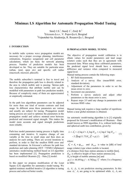
An automatic model-tuning algorithm is in [1] originally
proposed for Ericsson’s modification of Okumura – Hata
model known as 9999 algorithm. It is, without knife-edge
and spherical earth loss contribution, given by:
*
L = A + A log d + A log H
0
1
+ A log d ⋅log
H
2
[ H )] + g(
f ) [ dB]
−3.2 log(11.75
where:
*
A A + µ
2
m
eff
0
= 0 mob
and
mob
3
eff
−
(1)
µ is value in [dB] of lend
usage (clutter) type where mobile is located,
d is distance from base station antenna to mobile [km],
H eff is effective height of base station antenna [m],
H m is height of mobile antenna [m] and
g( f ) = 44.49log f − 4.78( log f ) 2
where f is a frequency
in MHz.
A 0, A 1, A 2, A 3 are prediction steering parameters. In this
case A 0
*
, A 1 are going to be optimised while A 2, A 3 are

assumed to be set to their default values, i.e. –12 and 0.1
respectively. H m and f are known from the actual
measurements. The tuning is then performed for one
clutter at a time.
Measured path loss can be obtained in [dB] for each
coordinate point by:
M
i
EiRP + G
A, i
− SS
measi ,
= (2)
where EiRP is emitted radiated power with cable losses
and antenna gains [dBi] taken into consideration and G A,i
is antenna masking gain for point i dependant on the
horizontal and vertical angles between base and mobile
station antennas. SS meas,i is measured signal strength for
coordinate point i. EiRP and G A,i are supposed to be
known from the actual measurement process.
For different clutter types, the sum of the difference
between predicted values and measured data will be
minimised and RMS error function will be as follows:
N
* 1
*
2
E( A0 , k
, A1,
k
) = ∑[
Li
( A0,
k
, A1,
k
) − M
i
] , (3)
N
i=
1
where N is number of measured points.
Equation (1) can be written in form
*
L i = A0 + A1
Bi
+ Ci
(4)
where
B = log , (5)
and
i
d i
C = A logH
i
2
eff , i
2
[ H )] + g(
f ) ⋅
−3.2 log(11.75
+ A logd
3
m
i
⋅logH
eff , i
−
(6)
For minimising E(A 0 * , A 1 ), the equation (3) is
differentiated partially with respect to A 0 * , A 1 . N
equations have to be solved:
i = 1:
i = 2 :
M
i = N :
*
A + A log d
M
0
*
A + A log d
0
*
A + A log d
0
1
1
1
1
2
N
+
+
C
+ C
C = M
N
1
2
= M
M
= M
1
2
N
. (7)
The overdetermined eq. (7) system can be written as,
⎡1
⎢
⎢
1
⎢M
⎢
⎣1
B1
⎤ ⎡ M
1
− C1
⎤
⎥ * ⎢ ⎥
B2
⎥
⎡A
⎤
⎢
M − C
0
2 2
× ⎢ ⎥ = ⎥
M ⎥ ⎣ A ⎦ ⎢ ⎥
1
M
⎥ ⎢ ⎥
BN
⎦ ⎣M
N
− C
N ⎦
*
The vector [ ] T
LS
or
a = A0
A1
can be obtained from
T −1 T
[ W W ] W Y
W × a = Y . (8)
a =
. (9)
III MINIMAX LS ALGORITHM
Coefficients A 0 * , A 1 in expression (9) give minimal mean
square difference (LS solution) between predicted pathloss
value and measured path-loss data. In the most
practical situations it is much better to have maximal
error values smaller.
There is number of minimax algorithms [4-7] that gives
solution of minimal maximal error. The most suitable is
minimax modified LS known as IRLS (Iterative
Reweighted LS) algorithm [5]. The algorithm is based on
an ides of modifying the Least Square method. IRLS
implements the windowing concept in LS algorithm, and
shows that the concept can lead to minimax mismatching
[5].
IRLS algorithm in time domain is given by
T
−1
T
[ W R(
j −1)
W] W R(
j −1
Y
a ( j)
=
(10)
IRLS
)
where j is iteration number and R(j-1) is a weighted
(window) error matrix:
and
[ r(
j 1) ]
R ( j −1)
= diag −
(11)
( j − ) ⋅e( j)
r( j)
= r 1 . (12)
e is an error vector given by
[ M − L , M − L , 2
− ]
e =
1 1 2
L,
M N
L N
. (13)
The weighted error which is included in the matrix R can
be understood as a corrective factor of the LS algorithm.
In every new iteration weights are innovated according
errors from previous iteration.
IV RESULTS
To verify proposed algorithm for automatic model tuning
RF field measurement carried out at many locations in
Serbia. Active base stations (BS) in “Telekom Serbia”
GSM mobile network are used as transmitters for signal
strength measurement. For path-loss calculation real BS
EiRP value is used while Heff and G A is calculated for
every measuremet point. Heff is calculated by relative
method. Sampling speed is adjusted according vehicle
speed (50 samples per sampling length of 40λ), in order
to smooth out the Rayleigh fading and reduce the
correlation between two adjacent samples [9]. Calibrated
receiver from the TEMS Investigation tool performs
measurement in the 0th time-slot at the BCCH
frequency. RF measurement results are together with
GPS coordinates stored in Signia files format and further
processed in Matlab.

In the tuning process maps with 100m and 20m digital
terain model (DTM) resolution have been used.
Route I is measured in the region of city Indjija. For the
open area estimated coefficients, standard deviation and
maximal/RMS error is given in Table 1. It can be noted
that maximal error is decreased while RMS error is
increased. In the figure 1 and 2 change of maximal error
and standard deviation in the itarative procedure is
shown.
A * 0 A 1
STD RMS
Error
Max
Error
LS 45.95 100.6 6.04 36.5 20.2
IRLS 47.31 101.0 6.04 38.0 18.4
Table 1 Estimated coefficients for the open area.
20.4
[dB]
20.2
20
19.8
19.6
19.4
19.2
19
18.8
18.6
18.4
0 5 10 15 20 25 30 35 40 45 50
Iteration Number
Fig. 1 Decrease of maximal errior in the iterative
procedure.
145
[dB]
140
135
130
125
120
115
110
105
iii
100
0 1000 2000 3000 4000 5000 6000 7000 8000 9000 10000
Sample number
Fig. 3 Comparison of mesured (i) and predicted path-loss
with coeficients obtained by LS (ii) and IRLS (iii)
algorithm.
Figure 3 shows path-loss measured on the route 1
compared with the path losses obtained by LS (dotted
line) and IRLS algorithm (solid line).
A * 0 A 1
STD RMS
Error
i
ii
Max
Error
LS 43.20 68.93 4.96 24.52 17.36
IRLS 44.17 80.55 4.96 27.1 14.56
Table 2 Estimated coefficients for the suburban area.
Route II is measured in the region of city Indjija but for
suburban area clutter. Estimated coefficients, standard
deviation and maximal/RMS error is given in Table 2.
Maximal error is decreased by 2.8 dB while RMS error is
increased by 2.58 dB.
[dB]
6.12
6.11
IV CONCLUSION
6.1
6.09
6.08
6.07
6.06
6.05
6.04
0 5 10 15 20 25 30 35 40 45 50
Iteration Number
Fig. 2 Standard deviation during a iterative procedure.
Not only RMS error and standard deviation are
important parameters for evaluation of the propagation
model tuning process. Maximal difference between
predicted and measured values is significant and has to
be minimised. In this paper algorithm for maximal error
value minimisation based on minimax LS (IRLS)
algorithm is proposed. It gives possibility to choice type
of error that will be minimised in the tuning procedure.
In some cases IRLS algorithm has a problem with
convergence. It will be investigated in the future. Also,
further research will be focused on automatic tuning for
all steering parameters defined in 9999 propagation
prediction model.
LITERATURE

[1] Ericsson Radio Systems AB, TEMS TM CellPlanner 3.4
User Guide, 2001.
[2] Y. Okumura, E. Ohmori, T. Kawano, K. Fukuda, ”Field
strength and its variability in VHF and UHF land-mobile
radio service”, Review of the ECL, 16, pp. 825-873,
1968
[3] Hata M., “Empirical formula for propagation loss in land
mobile radio service”, IEEE Trans. on Vehicular and
Technology VT-29, pp. 317-325, 1980.
[4] Haykin S.,”Adaptive Filter Theory”, Prentice Hall, New
York, 1986.
[5] Rapajic P. B., Zejak A. J., "Low sidelobe multilevel
sequences by minimax filter", Electronics letters, Vol.
25, No-16, pp. 1090-1091, 1989
[6] Zejak A. J., Zentner E., Rapajic P. B. "Doppler optimized
mismatched filters", Electronics letters, Vol 21, No. 7,
pp. 558-560, 1991
[7] Cavin R.K., at all,”The design of optimal convolution
filters via linear programming”, IEEE Trans. Geosc.
Electron., Vol. GE-7,No.3, pp.142-145,1969
[8] Digital mobile radio towards future generation systems,
COST 231 group Final Report, COST Telecom
Secretariat, COST@postman.dg13.cec.be
[9] Lee, W. “Mobile Communication Engineering - Theory
and Applications”, McGraw-Hill, 1998
Abstract: Propagation model tuning is time consuming
and iterative process. Automatic model tuning based on
LS algorithm is proposed in Ericsson’s TEMS
Cellplanner radio planning tool. In this paper we suggest
use of modified LS algorithm that decrease maximum
error of predicted signal without influence on standard
deviation compared to LS method.
AUTOMATSKO PODE[AVANJE PARAMETARA
PROPAGACIONOG MODELA PRIMENOM
MINIMAKSNOG LS ALGORITMA
Simi} I., Stani} I., Zrni} B.