Headphone Sound Externalization - TKK Acoustics

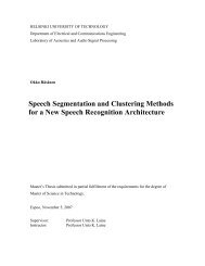
HELSINKI UNIVERSITY OF TECHNOLOGY
Department of Electrical and Communications Engineering
Laboratory of Acoustics and Audio Signal Processing
Toni Liitola
Headphone Sound Externalization
Master’s Thesis submitted in partial fulfillment of the requirements for the degree
of Master of Science in Technology.
Tampere, Mar 7, 2006
Supervisor:
Instructors:
Professor Vesa Välimäki (TKK)
Tapani Ritoniemi (VLSI Solution)

HELSINKI UNIVERSITY
OF TECHNOLOGY
Author:
Toni Liitola
ABSTRACT OF THE
MASTER’S THESIS
Name of the thesis: Headphone Sound Externalization
Date: Jan 23, 2006 Number of pages: 83
Department: Electrical and Communications Engineering
Professorship: S-89
Supervisor: Prof. Vesa Välimäki
Instructors: Tapani Ritoniemi, M.Sc.
Listening to the music via headphones using portable media players has become common
lately. If the sound is not properly postprocessed by headphone designated algorithm, it is
likely to be localized inside the head, making the stereo image unnaturally lateralized between
the ears and generally narrow.
Common headphone sound enhancing systems can be classified to three categories: simplified
spatial processing algorithms, HRTF-based binaural processing algorithms and virtual source
positioning algorithms. In this thesis all of these types are investigated and combined to find
one method that produces the aimed outcome of binaurally reproduced audio having better
’out-of-head’ localization when using the headphones.
Firstly, complicated systems having HRTF-processing followed by high spatial and temporal
accuracy room response modeling is evaluated. Later, reduction towards minimal system with
only simulation of most comprehensive physical cues are investigated.
As a result, simple and robust externalization algorithm is composed, which simultaneously
fulfills the preset standards of ’out-of-head’ sensation of sound and tonal pleasentness. The
algorithm uses primitive channel separation as the source modeling. The medium is characterized
as a virtual room of user defined size and properties. Special reflection rendering matrix
handles the realistic inclusion of spatial cues. Finally the listener part, which is also included
within the medium model, is approximated with contralateral diffraction characteristics that are
based on the measurements. The developed algorithms is also be applicable to varying types
of listeners and headphone equipment.
Keywords: Signal processing, Audio processing, Acoustics
i

TEKNILLINEN KORKEAKOULU
Tekijä:
Toni Liitola
DIPLOMITYÖN TIIVISTELMÄ
Työn nimi:
Headphone Sound Externalization
Päivämäärä: 23.1.2006 Sivuja: 83
Osasto:
Sähkö- ja tietoliikennetekniikka
Professuuri: S-89
Työn valvoja: Prof. Vesa Välimäki (TKK)
Työn ohjaajat: DI Tapani Ritoniemi
Musiikinkuuntelu kannettavilla soittimilla käyttäen kuulokkeita on nykyään hyvin yleistä.
Mikäli ääntä ei jälkikäsitellä kuulokekuunteluun soveltuvaksi, saattaa se paikallistua pään
sisälle aiheuttaen epäluonnollisen lateralisoitumisen korvien välille sekä kehnon stereokuvan.
Tyypilliset kuulokeäänen ehostusjärjestelmät voidaan jakaa kolmeen pääryhmään: yksinkertaistetut
tilaprosessorit, HRTF-pohjaiset binauraaliset algoritmit ja näennäisen äänilähteen sijoitusalgoritmit.
Tässä työssä kaikkia näitä lähestymistapoja tarkastellaan ja yhdistellään. Lopputuloksena
toteutetaan menetelmä, jonka avulla voidaan tuottaa pään ulkopuolelle paikantuvaa
kuulokeääntä.
Lähökohtaisesti tarkastellaan HRTF-pohjaista lähestymistapaa, missä käytetään tarkkaa fyysisen
tilan mallintamista. Myöhemmissä vaiheissa mallia supistetaan kohti vain kuulon kannalta
merkittävimpien ilmiöiden simulointiin sekä karkeaan tilamalliin jossa on vain kaikista olennaisimmat
piirteet. Eri lähestymistapojen pohjalta saadaan kuuntelutestien avulla lopputuloksena
nämä ehdot täyttävä ratkaisu, joka on toteutettavissa käytössä olevilla resursseilla.
Toteutettu menetelmä on suoraviivainen ja kaikenlaisille kuuntelijoille ja kuulokkeille pätevä
algoritmi, joka täyttää yhtäläisesti asetetut vaatimukset koskien äänen paikallistumista pään
ulkopuolelle sekä sen värin sensorista miellyttävyyttä. Lähdettä mallinnetaan alkukantaisella
kanavaerottelua parantavalla esikäsittelyllä. Siirtotien mallinnuksessa hyödynnetään
huoneakustista heijastusmatriisia. Huoneen piirteitä kuten fyysistä kokoa voi muunnella reaaliaikaisesti.
Kuuntelijamalli, joka sisältyy myös siirtotieosioon, toteutetaan jäljittelemällä pään
muodostamaa varjostuilmiötä, jossa apuna käytetään mittaustuloksia ja teoreettista mallia.
Avainsanat: Signaalinkäsittely, Äänenkäsittely, Akustiikka
ii

Acknowledgements
This Master’s thesis, Headphone Sound Externalization, has been done for VLSI Solution
Oy at Tampere, Finland. The work was carried out between October 2005 and February
2006 as a part of the software development project for Digital Signal Processors.
At first, I want to thank my instructor Tapani Ritoniemi for providing me the opportunity
to participate in this pioneering project and giving such appropriate topic for the thesis to
begin with. I could not have wished for the subject more interesting myself. I wish also
to thank to my supervisor Vesa Välimäki for his encouraging attitude, support and helpful
hints during the process.
Furthermore, I would especially like to thank Henrik Herranen for his indispensable aid
concerning numerous practical issues on multitude of occasions, and Erkki Ritoniemi for
his time and efforts in creating the real-time testing interface. My gratitude also goes to
the whole personnel at VLSI Solution for the creative and supportive atmosphere and their
sheer existence.
Finally, I would like to thank my fiancée Auli for her sympathy, love and patience.
Tampere, January 23, 2006
Toni Liitola
Sarastuspolku 5 B 13
FIN-01670 Vantaa
Finland
GSM +358 (0)40 538 7477
iii

Contents
Abbreviations
viii
1 Introduction 1
2 Psychoacoustic principles 3
2.1 Aspects of the audio signals . . . . . . . . . . . . . . . . . . . . . . . . . 3
2.2 Localization . . . . . . . . . . . . . . . . . . . . . . . . . . . . . . . . . . 4
2.3 Inter-aural cues . . . . . . . . . . . . . . . . . . . . . . . . . . . . . . . . 5
2.4 Tonal changes and HRTFs . . . . . . . . . . . . . . . . . . . . . . . . . . 6
2.5 Room response . . . . . . . . . . . . . . . . . . . . . . . . . . . . . . . . 7
2.6 Other cues . . . . . . . . . . . . . . . . . . . . . . . . . . . . . . . . . . . 8
3 Headphone sound characteristics 9
3.1 Binaural sound reproduction . . . . . . . . . . . . . . . . . . . . . . . . . 9
3.2 Binaural sound processing . . . . . . . . . . . . . . . . . . . . . . . . . . 10
4 Modeling virtual acoustics 12
4.1 Source modeling . . . . . . . . . . . . . . . . . . . . . . . . . . . . . . . 12
4.1.1 Source type . . . . . . . . . . . . . . . . . . . . . . . . . . . . . . 12
4.1.2 Channel expansion . . . . . . . . . . . . . . . . . . . . . . . . . . 13
4.1.3 Channel separation . . . . . . . . . . . . . . . . . . . . . . . . . . 15
4.2 Medium modeling . . . . . . . . . . . . . . . . . . . . . . . . . . . . . . . 20
iv

4.2.1 Physical approach . . . . . . . . . . . . . . . . . . . . . . . . . . 20
4.2.2 Modeling techniques . . . . . . . . . . . . . . . . . . . . . . . . . 21
4.2.3 Reduction of the model . . . . . . . . . . . . . . . . . . . . . . . . 25
4.3 Listener modeling . . . . . . . . . . . . . . . . . . . . . . . . . . . . . . . 27
4.3.1 HRTF-based listener modeling . . . . . . . . . . . . . . . . . . . . 28
4.3.2 Simplified cross-talk network . . . . . . . . . . . . . . . . . . . . 30
5 Implementation 34
5.1 Preprocessing . . . . . . . . . . . . . . . . . . . . . . . . . . . . . . . . . 34
5.2 Simulation of room acoustics . . . . . . . . . . . . . . . . . . . . . . . . . 37
5.3 Asymmetric ER models . . . . . . . . . . . . . . . . . . . . . . . . . . . . 41
5.4 Compressed ER . . . . . . . . . . . . . . . . . . . . . . . . . . . . . . . . 43
5.5 XT network listener model . . . . . . . . . . . . . . . . . . . . . . . . . . 44
5.6 User adjustable parameters . . . . . . . . . . . . . . . . . . . . . . . . . . 47
5.6.1 Sound field depth adjustment . . . . . . . . . . . . . . . . . . . . . 48
5.6.2 Sound field width adjustment . . . . . . . . . . . . . . . . . . . . 49
5.6.3 Spatial response adjustment . . . . . . . . . . . . . . . . . . . . . 50
5.6.4 Space size adjustment . . . . . . . . . . . . . . . . . . . . . . . . 50
5.6.5 Wall coloring adjustment . . . . . . . . . . . . . . . . . . . . . . . 51
5.6.6 Parameters hidden from user . . . . . . . . . . . . . . . . . . . . . 53
5.7 DSP requirements . . . . . . . . . . . . . . . . . . . . . . . . . . . . . . . 54
5.7.1 Preprocessor costs . . . . . . . . . . . . . . . . . . . . . . . . . . 54
5.7.2 XT network costs . . . . . . . . . . . . . . . . . . . . . . . . . . . 54
5.7.3 ER model costs . . . . . . . . . . . . . . . . . . . . . . . . . . . . 55
6 Analyzing results 56
6.1 Blind test . . . . . . . . . . . . . . . . . . . . . . . . . . . . . . . . . . . 56
6.2 Subjective evaluation . . . . . . . . . . . . . . . . . . . . . . . . . . . . . 59
v

7 Further improvements and studies 61
7.1 3-D sound mapping . . . . . . . . . . . . . . . . . . . . . . . . . . . . . . 61
7.2 Estimating RIR . . . . . . . . . . . . . . . . . . . . . . . . . . . . . . . . 61
7.3 Adaptive ECTF . . . . . . . . . . . . . . . . . . . . . . . . . . . . . . . . 62
7.4 Preprocessor improvement . . . . . . . . . . . . . . . . . . . . . . . . . . 62
7.5 Combining models with audio coding . . . . . . . . . . . . . . . . . . . . 62
8 Conclusions 63
A Octave code example 69
B C-code example 72
vi

¦
!
"
#
Abbreviations
¢¡
¢£
¥¤
¦¨§
©
£
¤
£
¤
Equivalent absorption area
Amplitude of the left channel
Amplitude of the right channel
Frequency
Sampling frequency
Z-domain transfer function
Power of the left channel
Power of the right channel
Time
Reverberation time
Input sample
Input sample left channel
Input sample right channel
Center sample
Modified input sample
Output sample
Z-transform variable
Absorption coefficient
Weight factor in cross-talk model
Azimuth angle
Elevation angle, Panning angle
Wavelength, Warping factor
Angular frequency
$
%
Preprocessing widening coefficient
AAC
APF
ASR
BRIR
Advanced Audio Coding
All-Pass Filter
Arithmetic Shift Right
Binaural Room Impulse Respone
DFT Discrete Fourier Transform
DSP Digital Signal Processor
DRIR Direct Room Impulse Response
ER Early Reflection
ERB Equivalent Rectangular Bandwidth
FD Fractional Delay
FFT Fast Fourier Transform
FIR Finite Impulse Response
FPGA Field Programmable Gate Array
HRIR Head-Related Impulse Response
HRTF Head-Related Transfer Function
IACC Interaural Cross-Correlation
IFFT Inverse Fast Fourier Transform
IIR Infinite Impulse Response
ILD Interaural Level Difference
IMDCT Inverse Modified Discrete Cosine Transform
ITD Interaural Time Difference
LPF Low-Pass Filter
LTI Linear Time-Invariant
MAC Multiply and Accumulate
MDCT Modified Discrete Cosine Transform
MP3 MPEG-1 Audio Layer 3
MPEG Moving Picture Expert Group
PRIR Parametric Room Impulse Response
RAM Random Access Memory
ROM Read-Only Memory
XT Cross-Talk
XMMS X-windows Multimedia System
vii

viii

Chapter 1
Introduction
Portable audio devices have become very common in the audio equipment markets lately.
The success of powerful audio coding methods, such as MPEG-1 audio layer 3 (mp3), together
with the increasing memory capacity of the portable media devices, this result is
perhaps quite understandable. One common factor for all portable audio devices, set aside
their small size and power consumption, is the fact their audio output device is primarily
headphones. Considering this observation, it is justified to pay special attention in the
processing of the sound signal to improve the perceptive quality when listened with headphones.
Anyone listening to the headphones has probably found the sound sometimes to be localized
in the head. The sound field becames flat and lacking the sensation of dimensions.
This is unnatural, awkward and even disturbing situation sometimes. This phenomenon is
often referred in literature as lateralization, meaning ’in-the-head’ localization. Long-term
listening to lateralized sound may lead to listening fatigue. Lateralization occurs, because
the information in which the human auditory system relies when positioning the sound
sources, is missing or ambiguous. The problem is emphasized on the recording material,
that is originally intended to be played via speaker systems.
The opposite phenomenon for the lateralization, and the title for this thesis, is the externalization
(see figure 1.1). Externalization means essentially ’out-of-head’ localization.
In the headphone sound externalization, sound is processed the way that the perception
about its position moves from the axis between the ears to outside the head. In this thesis,
powerful digital signal processing algorithms are utilized in conjunction with the theory of
psychoacoustics in order to achieve real time model which reduces lateralization property.
However, altering the sound usually introduces also tonal changes, which can be annoying
and even make the outcome worse than the original unprocessed audio. The tradeoff between
tonal and spatial accuracy is an optimization problem that this thesis essentially is
1

CHAPTER 1. INTRODUCTION 2
trying to give a suitable solution.
Headphone sound enhancement is generally divided in to three categories: simple spatial
processing algorithms, head-related transfer function -based binaural models and virtual
source positioning models. Head-related transfer functions, HRTFs, are measurement based
approximations of the effect which the human ear adds to the incoming sound. Externalization
systems based on HRTFs have been proposed in [18] and [26]. Their downsides
are generally the dependence of the individual ear shapes, twisting of the sound timbre and
computational burden. Lighter spatial processors are proposed in [12], [16] and [15]. Their
advantages are less exhaustive computational demands and independence of the listener.
However, they do not always work optimally in externalizing the sound either.
In this thesis, different approaches are investigated. The final solution can also be a combination
using multible approaches of the aforementioned categories. The initial approach
handles the problem with the source-medium-listener case where each part of this chain is
first studied thoroughly, and then a computationally effective model for each part is derived.
Alternative models are studied, compared, and tweaked to find the best parameters. Finally,
one appropriate model is applied to powerful modern 16-bit Digital Signal Processor, and
optimized with the subjective quality measures of psychoacoustical aspects. A digital signal
processor, DSP in general is a processor dedicated to operate with high data rates in real
time. DSP is a core of the more modern portable players.
Figure 1.1: Lateralization vs Externalization

Chapter 2
Psychoacoustic principles
2.1 Aspects of the audio signals
One of the key elements which separate audio signal processing from the general signal
processing is, that with audio, the ultimate receiver is always a human being. Therefore,
any operations made to the signal, should not only be investigated by traditional means, but
also at the viewpoint of perceptional abilities of the human auditory system.
Sound is usually processed in the time domain. The other very common domain is the
frequency domain, which is a result of an orthogonal basis function (for example Fourier)
transform, applied to discrete time and amplitude value approximations. When the psychoacoustic
aspects are added, we can further expand the transform domains in the way it
resembles more accurately the scale of humans perceptional capabilities. For example, doubling
the power of the audio signal does not double the loudness of the perception. Neither
does numeric inspection of the the frequency content always give clues to define the subjective
pitch to be perceived. The way these fundamental qualities of sound are percepted
by a listener is very nonlinear.
Several subjective measures have been formed with the help of listening tests, for example
such as phones and sones for the sound level. Perceived sound frequency has also many
different scales, some derived from listening tests, others having connections to auditory
models and physiological features of the cochlea in the inner ear. For subjective frequency
scales, most commonly used are the so called Bark, Mel or ERB scales [14], [37]. All
of them separate low frequency content more accurately than the higher one. The details
of these scales are not reviewed here, although they are considered throughout this thesis,
whenever judgments considering parameters of different schemes and parts of the model
are chosen.
3

CHAPTER 2. PSYCHOACOUSTIC PRINCIPLES 4
In the perception of sounds, certain effects such as frequency and temporal masking
changes the way a human is able to detect the sound compared to a device, such as microphone
for example. Temporal post- and premasking can make weaker sounds inaudible
with the presence of louder sound [14]. In frequency masking, some frequency content
of a single sound might be masked by another, louder content with relatively close central
frequency to the masked one. These effects are also kept in mind for the possibility of
exploiting them in some ways to gain good and computationally inexpensive solutions.
While the core of this thesis is neither in the theory of room acoustics, it is still one part
of the source-medium-listener approach. The medium, transition channel in which humans
are accustomed to percept the sound, is usually a space of some sort. Listening rooms,
concert halls and outdoors are potential spaces, just to mention few. Subjective measures
of listening room characters have been introduced, even with formulas approximating the
magnitude of these phenomenona [14],[32]. The most important subjective room character
measures considering this thesis are the energy of direct sound, the character and quantity
of the early reflections, especially horizontal ones, and the reverberant field behavior.
In the literature, several attempts to model the human auditory system with these phenomena
have been formed. One of the latests presented by Pulkki et al. would fit well in
objective evaluation of some aspects of this thesis [29]. However, even with these models
of the human auditory system and definitions for subjective measures, it is not possible to
override subjective quality tests in order to measure some characteristics of the perceived
sound. Not even the simplest decision whether the sound quality is improved or degraded
after some particular process. In this thesis, this has been occasionally quite a challenge,
since finding suitable test subjects to frequently raising need of them was a continuous
problem during the whole process of research and testing.
2.2 Localization
The main psychoacoustic focus of this thesis is on the theory of the localization in human
auditory system. Localization is the term for the process involving the auditory system of
the brains, where the spatial position of the sound source is estimated. The auditory cortex
at brains has a task to analyze several aspects of the heard sound signal.
There are several ways a listener can decide the direction of incoming sound. Many of
these rely on the fact humans have two ears. However, even persons with one functional
ear can hear the direction of the sound, although with drastically reduced accuracy. Some
directions of the sound tend to systematically be localized incorrectly, whereas other directions
are just simply very inaccurate [11]. As a rule of the thumb, the localization is
best in the frontal field, and worse at the sides and rear. In the next sections, different cues

CHAPTER 2. PSYCHOACOUSTIC PRINCIPLES 5
contributing the process of localization are investigated.
Localization cues are crucial considering the aim of this thesis, as they are the main
reason (or actually lack of them) why the lateralization appears in headphone listening.
The theory of localization can be viewed as the listener part in the source-medium-listener
approach.
2.3 Inter-aural cues
Inter-aural cues refer to the sound signal difference between the ears. Inter-aural cues are
the most important means for the localization.
In the listening tests ([29],[38]) it has been revealed that the pressure level difference
between the ears, Inter-aural Level Difference (ILD) is the most important single cue for
localization. When the sound arrives from the transversal plane with non-zero azimuth, it
has different level in each ear. The shadowed ear, also called contralateral (opposite sided)
ear, has naturally suppressed sound image compared to the unshadowed, which might be
referred as ipsilateral (same sided) ear. ILD has a dictative role when localizing higher
frequencies. A technique to model relationship between ILD and frequency is clarified in
the next section.
The other very important property to deal with localization is the Inter-aural Time Difference,
ITD. The shadowed ear has longer distance to the sound source and thus gets the
sound wavefront later than the unshadowed ear. The meaning of ITD is emphasized in the
low frequencies, which do not attenuate much when reaching the shadowed ear compared
to the unshadowed ear. ITD is less important at the higher frequencies, because the wavelength
of the sound gets closer to the distance between the ears. It has been observed that
on sound signals under 400 Hz, the fluctuation of ITD at 3-20 Hz rate has a role in forming
the envelopment and believable externalization of sounds [5].
ITD does not change much when the distance to the sound source is lengthened, but ILD
has differences when comparing its near field behavior to far field behavior. In this sense
the near field refers to distances closer than one meter [14]. For this reason, no further study
is necessary considering the design in this thesis. Near field behavior of the sound is not
interesting here, because the physical model under construction is derived to imitate real
world listening circumstances of a typical far field situation.
Inter-aural cross correlation (IACC) contributes also to the localization of hearing. IACC
describes the signal differences between two ears more accurately. ITD can actually be seen
as the distance between two maxima at IACC sequence. ILD could be roughly considered as
a scaling factor of IACC. IACC is helpful when there are many sound sources in different
locations. Auditory system can localize individual sources with the help of IACC. If the

CHAPTER 2. PSYCHOACOUSTIC PRINCIPLES 6
localization cues of only one sound source are considered, IACC gives little additional
information compared to sole ITD. Cross-correlation is also as heavy a process that it is
best to avoid it in real time systems. Further properties of IACC are more investigated in
the [27], but they have no direct implementation in the DSP algorithm of this thesis. That
is partly because of the computational complexity and less ephasized role compared to ITD
and ILD.
2.4 Tonal changes and HRTFs
As mentioned earlier, the inter-aural cues are the most important factors in the localization.
Yet a single ear can also contribute to the decision of the incoming sound direction. This
is crucial when the sounds come from median plane, for example above the listener, but at
equivalent distance from each ear. ITD and ILD can not help in the cases like this, as they
are equal. Some other means for localization must be then applied.
The parts of the outer ear such as the pinna and the concha, and even the parts of the human
body, such as shoulders, will act as acoustical filters to change the phase and amplitude
of the sound depending on the direction. Different angles introduce different resonances and
anti-resonances to the sound pattern arriving at the basilar membrane of the inner ear. The
response of the ear with different azimuth and elevation is called the Head Related Transfer
Function, (HRTF). Sometimes it is also referred as Head Related Impulse Response
(HRIR), which is the time domain equivalent of the frequency domain presentation HRTF.
The HRTFs are relatively new concept in audio processing. They have been extensively
investigated for applications like 3-D sound and auralization algorithms. One of the most
recent and rather profound introductions to the HRTF-related discussion can be found on
[31].
HRTFs are also slightly dependent on the distance. Because of the air absorption, certain
frequencies are attenuated more than the others, as the sound waves travel trough the air.
Shadowed ear HRTF differs radically from that of the unshadowed ear. The bigger the
azimuth angle, the more shadowing the head will cause. Sound wave diffusion makes low
frequencies less exposed to the HRTF alternation [8],[9]. All these dependencies and their
relations to HRTFs can be exploited in the process of designing a DSP algorithm to divert
auditory system.
The accuracy of the localization in human auditory system is highly dependent on the
sector it is originating. Sound from sides is localized with a poorer accuracy than sound
from the front. The special case of angles where both ITD and ILD are same, is called a
cone of confusion. For example, it is sometimes hard to figure out if the sound came from
azimuth 45 degrees, or from azimuth 135 degrees, as the inter-aural cues are same for those

CHAPTER 2. PSYCHOACOUSTIC PRINCIPLES 7
angles.
While accurate enough for the most tasks, the auditory system has a tendency to make
radical mistakes in some sectors. For example, sometimes sound originating from behind is
localized to the front. The sound coming above and behind is systematically localized too
low [14]. These errors are worth mentioning but their deeper analysis is skipped for their
irrelevance considering the problem at hand. A common factor for all localization errors is
that ITD and ILD are ambiguous or zero. In most errors, more cues are needed to make the
position of the source distinguishable. Next sections will introduce the rest of the cues, and
also comment whether they can be included in the model to be designed.
2.5 Room response
Humans seldom listen to the sounds in anechoic chambers or in places where there are no
reflecting surfaces. Therefore, the listening space affects the localization as well. Listening
space is one of the most important elements in evaluation of the distance of the sound
[34],[14]. The localization is based heavily on the rule of the first wavefront, the direction
in which the sound comes first. This phenomenon is usually referred as the precedence
effect, or Haas effect. As the direct path from origin of the source is also the shortest
route between it and the ear, this is understandable. Any sound pulse arriving later than
the first wavefront, but having relatively same shape must be a reflection. Localization in a
room is more accurate on the transient type sounds. In steady state sounds, the reflections
are confused easier with the directs sound, making the localization harder. It has been
suggested that in these situations, central processes based upon plausibility of localization
cues are utilized [8], [9]. The relation of the direct and reverberant sound, called acoustic
ratio (AR), is in fact claimed to be the most important factor in out-of-head localization
considering headphones [41].
Reflection characters provides information about the space to the auditory system. Small
spaces vary from larger ones in the sense of reflection timings and the time it takes from
all reflections to attenuate below threshold of hearing. As mentioned earlier, reflective
characteristics contribute to the subjective sound quality. The desired room response is as
important as the modeling of the listener. It should be easier to trick the auditory system to
localize the sound out of the head, if it seems to have cues referring to its distance.
The difference between reflection and reverberation is that a single reflection can be
observed as a separate sound image with somehow perceptible direction [32], whereas reverberation
is omni directional radiation of the room. The room response is modeled in
this thesis as the combination of a few early reflections and late reverberation. Detailed
description of the DSP implementations are derived later. One way to remove ’out-of-head’

CHAPTER 2. PSYCHOACOUSTIC PRINCIPLES 8
localization is to introduce a virtual room, a natural medium for the sound waves to propagate.
While not trying to render the acoustics of the concert hall or such, decent modeling of
the room has showed to result better ’out-of-head’ localization in several implementations.
However, exaggerated spatial processing usually ruins the clarity of the sound, so subtle
approaches are favored here.
2.6 Other cues
Some localization cues are based on the usage of hearing in conjunction with some other
sensory system. Typically, a listener will direct the head toward the interesting or intimidating
sound. This has led to the co-operation of visual cues with the auditory cues. It
has been shown that auditory and visual systems have interconnection at the brain, and thus
they influence to each other [42]. When a person sees the sound source, rather accurate
localization takes place. This could be proposed to be one of the reasons why front sector
localization is dominantly accurate over other sectors, it has had the best training and feedback
mechanism. Also, this is one of the problems in headphone sound listening. The fact
that there are no visible sound sources (such as speakers) makes it hard to believe that the
sound could originate from a specific location in the field of vision.
In the event of blurry sound localization or otherwise spontaneously, a listener is likely
to turn the head slightly during listening. This will alter the characteristics of all listening
cues, ITD, ILD and HRTFs as the incoming angle of the sound will change. This will also
produce more precise sound localization. Although neither of these cues can be exploited
in the DSP implementation of headphone sound manipulation, they were worth mentioning
to enlighten some of the weaknesses of any binaural model. They cannot be easily dealt
with and must therefore just be tolerated. A solution to the head turning issue is suggested
and overviewed in the chapter 7, but it merely is reasonable in the portable systems and
casual listening. Head turning is one of the most useful means of separating front and rear
originated sounds, because of the opposite reaction in the ITD/ILD balance.
Other parts of the human body are also exposed to mechanical vibration of sound waves
beside the fluid in the cochlea. Especially low frequencies with high intensity can be felt
in body and skull structures. These of course contribute little to the accuracy of spatial
localization, but being signs of such massive intensity, they might help to believe that the
source is inevitably external.
In the doctoral thesis by Jyri Huopaniemi [11] it was summarized that exaggerating certain
cues, such as ITD which expands virtual size of the head, localization seemed to improve.
Adding these super-auditory cues is also considered in this implementation, where
no individual HRTF measurement database can be accessed to improve spatial resolution.

Chapter 3
Headphone sound characteristics
3.1 Binaural sound reproduction
Before entering to the details of the physical modeling, some of the issues always present at
the headphone listening should be introduced. The ideology behind binaural technology is
based on the fact that humans have two ears, so in principle every sound image appearing in
the real world can be imitated just by creating the appropriate sounds directly to ears. This
means that any sensation of directions and spaciousness should be possible to be recreated
using headphones or cross-talk canceled speakers.
The task is perhaps easier using headphones, because the cross-talk canceled speaker
setup is even at its best highly dependent on the listening position. This intersection of the
cross cancelling waves is known as the ’sweet spot’. On the other hand, lateralization does
not occur in the speaker reproduction. The goal of this thesis is to achieve some benefits of
speaker audio in that sense.
Although 3-D sound systems are becoming more and more popular in audio technology,
especially in electronic games and movies, stereophonic sound still dominates in the music
industry. Stereophonic sound consists of two channels, which are independent and often
labeled left and right channel. Music is usually not recorded using an artificial head, but
instead high quality microphones. The consequence is that the music is not ideal to be
reproduced via headphones, not at least in the terms of its fidelity to the original capturing
situation. To put it more simply, the music recorded using two microphones and then played
back using headphones cannot be identified with the situation where the listener would be
actually sitting in the place of microphones during the recording.
9

CHAPTER 3. HEADPHONE SOUND CHARACTERISTICS 10
3.2 Binaural sound processing
The key issues behind lateralization are the absence of the cues always present in real world
sound sources, including speaker reproduction. Absence of cross-talk phenomena such
as IACC, its simplified special cases like ITD and ILD, and the absence of human body
reflections (HRTF characteristics) together with no spatial response product to the ’in-thehead’
localization as brains do not have to deal with similar inter-aural sound pattern with
any real life sound sources. When the auditory system does not have any particularly good
reason to localize the sound source to any point, it is localized to the axis between the ears,
inside the head.
Many musical scores have two-track audio material that has been recorded with the use
of two microphones, with some distance between them. Or perhaps the audio mixer has virtually
panned source instruments with amplitude panning that would give the desired result
when reproduced with speakers. This material has the potential of becoming inexplainably
disturbing while listening it trough headphones, as its has all the features listed above. The
signals that arrive to ears, are describing an unnatural and impossible field of sound.
With simple comparison to the visual sensory system, the described situation could be
compared to the case where the visual image to the left and to the right eye would be as
seen from two totally different angles. The brains could not unify them to a perception of
some natural space. This is basically what happens in the auditory system too.
Also acoustical coupling of the headphones with free air is different from other sound
sources. Here one of the most encouraging features of the headphones steps in. The benefit
of the independence of the surrounding space. Any room will suit equally well for the
immersion created by processed headphone signal. Only the background noise level should
be tolerable, although even that is slightly attenuated in some headphone systems. In short,
the surrounding space does not much interact with the headphone sound, and the headphone
sound does not either much interact with the space. This makes it an ideal listening device
in situations where low sound pressure levels are appreciated, such as night listening in tight
quarters.
It can be observed that artifacts of lossy audio coding and other undesired effects in
recordings are more present in headphone listening, partially because the lack of the compensating
effects of the room response, such as temporal masking. Only the ear canal
resonance is present in the audio image of the headphones. So the auditory system in headphone
listening tend to be more unforgivable to the glitches caused by frequency component
reduction of lossy coding, like DCT cropping based methods (MP3, Ogg Vorbis, WMA).
In principle, it would be possible to deal with all these problems in the recording and
preprocessing of the sound clip, whatever its format is. But if this were done, the same

CHAPTER 3. HEADPHONE SOUND CHARACTERISTICS 11
sound clip would not be appropriate to be played back from speakers anymore, as all these
virtually added cues would be generated again concretely resulting odd set of mixed cues of
localization. Therefore it is wise to implement a real-time process that can add these effects
afterward, if the headphones are used to listening purposes.
The task to remove or at least weaken the lateralization effect without reducing the perceived
quality is not as easy as it may seem. One can be under impression that making an
algorithm for two channel would be easier than for example making an algorithm to produce
five channels through headphones. This impression is false all the way. Five channel
version of the headphone sound is easier in the sense that spatial information is known beforehand
from the given set of channels. In the two channel case, all information of the
audio is in only two channels. Where the sound originates in the two channel case is not
explicitly defined by the audio track. Also, any room response included in the material is
essentially just short of proper dimensions.
It can be argued that stereo processing is more challenging process than delivering 3-D
sound to headphones, which is in the simplest case just a problem of finding a set of good
HRTFs. Furthermore, subjective results derived by Lorho et al. pointed out that most headphone
sound enhancing and externalizing systems so far designed only made the perceived
sound quality poorer than the original unprocessed one [19] . The anti-lateralization system
is hardly justified, if it reduces the sound quality too much. It is difficult to develop a sound
enhancing system in the first place, because a human is so adaptive to certain effects within
any sound.

Chapter 4
Modeling virtual acoustics
4.1 Source modeling
Source modeling in this DSP implementation is straightforward. Because the source signal
is already assumed to be captured in the audio content to be reproduced, no assumptions of
what instruments and sounds it contains can be made. As the typical listening conditions
were aimed for virtual acoustics of this implementation, the sound of the stereo channels left
and right were fixed to originate from two or more virtual speakers, yielding some azimuth
and elevation angles. Azimuths up to 90 degrees for the right speaker and -90 degrees
for the left speaker with several elevations are sensible. The azimuths could be chosen to
correlate real world listening room layouts.
4.1.1 Source type
It should also be noted here that the goal is not directly to model a certain source, like a
human speaker or an instrument. Instead, a good reproduction environment is the emphasis.
Say, listening to the music with high end speakers in a medium sized listening room is more
like the target situation.
In typical recordings, the stereo image is created with panning the source signals between
the left and the right channels. The simplest panning methods are linear panning and power
complementary cosine/sine (also called tangent) and sine panning. Pulkki and Karjalainen
derived more sophisticated vector based amplitude panning, which more accurately considers
the auditory weighting of the inter-aural cues [28] . Panning is essentially mixing
a monoaural signal into two channels, each having some portion of the total energy of the
original signal. When reproduced from loudspeakers, panned signals are localized according
to their relation of power in each of the channels. In perceptional position of the source
12

CHAPTER 4. MODELING VIRTUAL ACOUSTICS 13
were measured for the two simple and widely used panning algorithms. The arguments of
the trigonometric functions in the formula are in degrees. &£ is the gain of the left channel
and ¥¤ the gain of the right one.
(')'*,+)- '/.¨021 13. 547698¨:@698¨:AB,C)ED
¢£GFH ¥¤
¢£JI ¥¤ 2K (4.1)
(')'*,+)- '/.¨0L1 1M. N4PORQS: ;= > 698¨:AB,C)ED
¢£GFT ¥¤
¢£JIU ¥¤ K (4.2)
The arguments of trigonometric functions are in degrees.
From these measurement based results, neither cosine/sine (tangent) nor sine -panning
deliver exactly the intended directions to the sound to be mixed, but tends to be too wide
on two speaker arrays [6]. Perceived sounds are localized too far to the direction channel
having most energy. More about different panning techniques and how the auditory system
relates to them in [27], [6] and [28]. For the scope of this thesis, it is enough to know that
this kind of preprocessing exists, so that it can be taken to account as the source signal
property.
Adding artificial reverberation and echoes after the recording is also possible in the mixing
stage. The problem of the artificial reverberation is that when it is only on the two audio
channels, it cannot easily be separated from the original dry sound. Artificial reverberation
tends to also sound like it is coming inside the head when using headphones.
4.1.2 Channel expansion
One variation of the two-speaker source configuration was inserted as an option to the
model, a three-speaker setup. In addition to the left and right speaker, a virtual center
speaker was inserted. Center speakers are widely used in surround sound systems. Here,
the role of the center speaker is to collect all the mono-aural audio and handle it separately
from the left and right channel. This could be filtering it using HRTF filters with azimuth
0, as in HRTF-based models, or something else.
Moreover, adding a center channel leads to widened azimuths on left and right channel,
which makes the width of the virtual source positions wider on the front. Center channel
input is defined as the mono-aural part of the input sound. It should also be noted that if
the sound is modeled to virtually come from one center speaker compared to amplitude
panning of two speakers, the cross-talk between the ears differs, as there is no ITD. In the
two speaker setup, mono-aural sound produces a feed-forward comb-filter effect, as the
signal propagates to an ear from two paths, once from the closer speaker and second time
from the cross-talk route. This is illustrated in the figures 4.1 and 4.2. Mono-aural part
can be estimated from left and right channel. For computationally lightest algorithm, the

CHAPTER 4. MODELING VIRTUAL ACOUSTICS 14
extraction is a mere average of the signals. This can be expressed with a simple equation
4.3:
V4XW
Y
£ I ¤
(4.3)
It can be assumed that the mono-aural part is the center channel. The mono-aural part
has the same amplitude in both left and right channel. If these channels had the same signal
component, it is included twice, having double amplitude (quadraple power) compared to
the signal portions that existed only in the left or only in the right channel. This computation
is also easy to implement with DSP, as it requires only one summation, and halving can be
implemented by shifting the bits arithmetically to the right. Better yet, there is no need
of division by variable number, as there would be in some of the most common two to N
channel upmatrixing surround sound processing schemes.
Pressure
Left ear
Time
Pressure
Right ear
Time
Figure 4.1: Mono-aural audio in 2 speaker setup, speakers produce same signal

CHAPTER 4. MODELING VIRTUAL ACOUSTICS 15
Pressure
Left ear
Time
Pressure
Right ear
Time
Figure 4.2: Mono-aural audio originating from one center speaker
4.1.3 Channel separation
The simplest way to extract left-only and right only signals, is to subtract their difference to
one channel, as in 4.4 and 4.5 [11]:
£ V4 £ I £ F ¤
(4.4)

Y
I
I
CHAPTER 4. MODELING VIRTUAL ACOUSTICS 16
£
is the left channel input sample at time instant n, and ¤
input sample at the same instant.
¤ V4 ¤ F £ F ¤
£
and
¤
(4.5)
is the right channel
are the corresponding left-only and right only
signals. Without center channel inclusion, this kind of widening de-emphasizes the low
frequency content, as low frequency component producing instruments are highly concentrated
to the center when mixing. If the signal is center panned, its difference is zeros. This
widening is rather brutal in other aspects as well, since it requires a lot of downscaling. If
for example, the left channel has value 1, and right channel has value -1, the summation
of the difference would produce amplitude 3. To avoid the possibility of clipping, scaling
with 1/3 would be required, making the processed sound having attenuated over 9 dB compared
to the original signals. Also, amplitude panned signals would cause inverted signals
between the channels as early as possible.
If, for example, the left channel had a signal with amplitude 0.95, and the right channel
had the exactly same signal with amplitude 0.32, the mixer had probably tried to insert the
sound source heavily to the left. This situation is realistic in cosine panning, where the
C_ I Y _ba
sum of the Z\[^] Z\[^` W squared amplitudes is constant. (here, ) But the algorithm
would produce to the left channel output an instant amplitude value of 1.27 and for the right
channel value -0.32. Although the source is still on the left side as intended, its phase is
inverted on the right, shifted ced by . This is not a desired effect, because off-phase signals
sound quite dissensible when listened.
To prevent this, or at least making the problem less probable to pop up, slight modifications
to the equations above were tried. A widening factor W was defined. W has values
between 0 and 1, 0 meaning nothing is done, and 1 leading to the exactly same process as
in equations 4.4 and 4.5.
£ V4 £ I % Df £ F ¤
(4.6)
which can be simplified to:
¤ V4 ¤ F % Dg £ F ¤
(4.7)
£ (4h
W
(4.8)
%i £ F %j ¤
¤ V4h
W
(4.9)
%i ¤5F %j £
Now, the phase inversion point is shifted to farther away. The result with different widening
factors W, can be observed from the figures 4.3 to 4.6.

CHAPTER 4. MODELING VIRTUAL ACOUSTICS 17
Signal power / % max
100
80
60
40
20
Left channel
Right channel
0
0 20 40 60 80 100
Left bias / % max
Figure 4.3: Original panning, no widening (W=0)
Signal power / % max
100
90
80
70
60
50
40
30
20
10
0
0 20 40 60 80 100
Left bias / % max
Left channel
Right channel
Figure 4.4: Widening effect and phase inversion point, W=0.125
From the same figures, it can also be concluded, that even with the widening factor
W=0.25, the left biased signals are pushed more to the left quite efficiently. Another benefit
of using low widening factors is the scaling rule. With widening factor W, scaling by
=
_9l =3k
is required to make the output limited to unity. Thus, with W=0.2, already downscaling by
1.4 is enough to keep the output maximum as in original signal. In practice, scaling can also

CHAPTER 4. MODELING VIRTUAL ACOUSTICS 18
Signal power / % max
100
80
60
40
20
Left channel
Right channel
0
0 20 40 60 80 100
Left bias / % max
Figure 4.5: Widening effect and phase inversion point, W=0.25
Signal power / % max
100
90
80
70
60
50
40
30
20
10
0
0 20 40 60 80 100
Left bias / % max
Left channel
Right channel
Figure 4.6: Widening effect and phase inversion point, W=0.5
be neglected, risking the signal to clip. In actual listening, clipping seemed to happen only
rarely, and even then, it was not possible to hear any distortion. Therefore, it is tempting to
forget the scaling completely in order to preserve the same volume in the processed sound
as in the original.
If the center channel is not handled with HRTF filtering, it can be kept in stereo and

W
W
W
W
I
CHAPTER 4. MODELING VIRTUAL ACOUSTICS 19
manipulated with the contrary preprocessing for center left £
and center right ¤
:
£ (4m
(4.10)
F %i £ I
%n ¤
¤ V4h
(4.11)
F %i ¤ I
%j £
This kind of processing obviously makes the original stereo signal having more center
panned appearance, as the left and right signals are mixed together with weighting W. If
W=0.5, the signals are exactly same, making the stereo-center signal exactly monophonic.
The benefit of this contrary preprocessing for obtaining the stereo center is that summing
the true left
£
with the center left < £
gives:
(4.12)
£JI
£ 4
(4.13)
4hop
F %i £ I %q ¤ Mr I op
%i £ F %n ¤ Mr
4 Y £
(4.14)
Which is the scaled original left channel. Similarly for the right channel, the summation
produces the original right signal. If nothing would be done to the true left and right signals
or to the centered left and right, the preprocessing would not do anything but scale, if the
left signals are added as shown. The difference arises when the signals are treated diverged
ways prior to the addition.
Once the decisions of which part of signals are fed to left, right and center channel, the
system can be expanded to 3 (or 4 in stereo center) virtual speaker setup. Center channel
can directly be simulated in HRTF-based model by appropriate HRTF filtering, just like left
and right. In more stripped version of the model, the left channel handling also differs from
the true left and true right channel signals. Room response of the center channels can also
be tweaked, as the angles and delays of the reflections are different. This was also taken
account on the medium modeling, which is the topic for the next section. It should be noted
here that although the methods above give really poor channel separation, the requirement
for computation is so minimal that leaving it out does not make much difference in the
implementational costs. The effect of this mild widening is barely audible, if nothing else
is done. However, when later part of the models, such as medium model and listener model
are integrated with this simple source preprocessing technique, the effect pops out resulting
in better overall algorithm. It removes the narrowing effect caused by cross talk filters,
and also makes the artificial stereo reverberation more suitable for the implemented room

CHAPTER 4. MODELING VIRTUAL ACOUSTICS 20
model. There are a lot of more complicated and sophisticated stereo widening algorithms,
as also reviewed in [11].
4.2 Medium modeling
More important than the source, is the medium to achieve externalization. To model a
natural environment, some basics of room acoustics are required. Every real space adds
reflections to the direct sound. The modeling of the space can be seen as an attempt to
model the room impulse response (RIR).
4.2.1 Physical approach
The main RIR modeling classes can be divided to wave-based and ray-based [11]. In the
wave based method, spaces are modeled with for example meshes formed up of nodes.
The spatial density of the nodes sets limits to the highest frequency which behavior can be
approximated. Wave-based method can get quickly complicated in terms of computation
power. For the real-time application, they might be way off the budget. The other method,
ray based modeling, assumes that sound waves propagate in space as rays. This is basically
assuming the sound would reflect and behave like directional light beam would, for example.
Diffusion and diffraction are both neglected in this technique. One way to model the
reflections is the source mirroring where the reflection is viewed as another source, outside
the listening room [35], [11]. In this technique there are two main phases: finding the position
of the mirrored source, and deciding whether it is visible to the listener at point of
interest.
Materials in the listening room absorb sound energy, leading to the decaying impulse
response of the room. Materials absorbs the different frequencies unequally. Absorption
and reflection coefficients of different materials are usually documented in octave bands.
As generalization, the decaying can be seen as a low-pass type, because generally higher
frequencies are attenuated more quickly than the lower ones. The time it takes for a sound
to attenuate 60dB is often referred as the reverberation time. Different formulas to calculate
reverberation time with given room parameters have been introduced, perhaps most famous
of them being the Sabine’s formula. Sabine’s formula 4.15 gives a rather good estimate in
the scope of this particular application, where no specific room is indented to imitate. The
reverberation time e depends on the room volume s
in cubic metres, and total equivalent
absorption area ¥¡ in quadratic metres, which can be obtained as a sum of all absorbing
surfaces multiplied by their corresponding absorption coefficient.

D
s
CHAPTER 4. MODELING VIRTUAL ACOUSTICS 21
4
Z\[ WLt\W
¡ (4.15)
Also the possibility of no late reverberation is considered, as in round robin test by Lorho
et al. [19] it was observed that reverberation does not necessarily improve the overall subjective
quality. Too noticeable reverberation is detected as an effect, and therefore is not
quite the point of this study. In this thesis as well as generally, the difference between reflection
and reverberation is that reflection is a discretely modeled echo, with predefined
incoming angle and delay. A reflection has a certain direction. Reverberation is not this
detailed, but rather an estimate of the envelope of the magnitudes of the reflections with
respect to time. On top of that, spacing between reflections is sparser, as the sound has not
yet spread all over the listening space. The spacing of the sound pulses grows as time goes
by from the excitation.
Sound naturally attenuates with the distance in 1/r sense, if a spherical radiator model is
used. Also the air absorption is important when modeling large spaces with large distances
between the sound sources and the listener. The latter of these phenomena have been intentionally
left out of the system to be designed, as the desired model for medium is not
considered to be large enough to demand it. Air absorption is in addition questionable,
since it tonally colors the sound, and this is tried to be generally minimized.
4.2.2 Modeling techniques
A two-part room acoustical model was chosen as one test case to the implementation. The
early reflections are modeled as directional reflections coming from predefined direction
and delay. The temporal spacing of these reflections are chosen with the prevention of
undesired flutter echo in mind. The directions are chosen to model somewhat realistic
geometry of a listening room, but also subjective effects of lateral reflections are not forgotten.
In HRTF-based localization modeling case, early reflection simulating directional
HRTF filters are integrated with the simplified material absorption character of the reflector
material of the virtual room. In reduced cross-talk network design, early reflections are
added as low-pass filtered replicas of original signal, but with ITD, delay and magnitude
corresponding to azimuth value of a particular reflection.
As mentioned earlier, reflections can be considered as virtual sources in ray based model,
located in the virtual rooms derived by mirroring the real (in this case also virtual) room.
This way it is easy and intuitive to quickly gain azimuth and elevation angles, distance and
delay of the first reflections that have bounced via a surface wall or two. In figure 4.7,
typical example of finding reflections that have reflected of one or two walls in transversal
plane is portrayed. The solid rectangle is the loudspeaker and the circle is the listener.

D
CHAPTER 4. MODELING VIRTUAL ACOUSTICS 22
Table 4.1: Example ER matrix of the virtual Room
Azimuth / degrees Delay / m Relative gain
49 1.37 0.362
9 1.95 0.279
8 2.54 0.220
-60 2.69 0.209
34 2.86 0.156
31 3.37 0.132
-45 3.90 0.122
-132 4.33 0.099
Horizontal and vertical lines are walls of the listening room. Dashed rectangulars are the
virtual sources, whose arriving direction can be concluded from the dashed arrows. The
length of the arrows are comparable to the delay of the reflection. The number of walls the
arrow travels trough, is the order of reflection.
As a tool to design rooms, Octave function was written to produce a special ER matrix,
which consisted of all interesting data considering the first nine early reflections (see Appendix
A). In the table 4.1 there are output values for the typical listening room. As input,
the function took physical parameters of the room, such as its dimensions, reflection coefficients
and placement coordinates of the speaker and the listener. For output, the function
gave a matrix having delays of the reflections in meters, their relative magnitude compared
to the direct sound, and azimuth angle, which could be positive or negative (reflection came
from the other side of the room than speaker). The values of the example room in table 4.1
are for the right speaker. The values for the left can be achieved by mirroring the azimuths.
The speakers in the example were positioned to 17 degrees to the left and -17 degrees to the
right, which are the azimuths of direct sound rays. Floor reflection is excluded.
In the figure 4.8, physical distances of the listening room are labeled. Using the ray-based
approximation of the figure 4.7, the physical properties of the first reflections can expressed
with the help of comprehensive trigonometric formulations. A parametric room impulse
matrix can be formed, which expresses the relative distances from the virtual source to the
listener. ` ` The PRIR-matrices of the nine closest virtual sources of the rectangular room
(direct path and 8 transversal reflections) are:
Positional width difference matrix W:

y
y
y
y
y
y
{
{
{
y
{
{
{
y
y
I
I
I
y
y
CHAPTER 4. MODELING VIRTUAL ACOUSTICS 23
Figure 4.7: Image-source method on rectangular room
Y % F }
€
W 4vuwxzy|{ I~}
‚ (4.16)
Fg}
Fg}
{ y|{
y|{
I~}
Y % F }
y|{
{ y|{
Positional length difference matrix L:
y {
y|{
I~}
Fg0
Y % F }
y {
{ y {
L 4juwx y £JI~}ƒ£
‚ [ (4.17)
£JI~}ƒ£
£JI~}ƒ£
€
£GFg}ƒ£
£GFg}ƒ£
£GFg}ƒ£
The azimuth of the virtual source:
£…F Y
}ƒ£„I
£…F Y
}ģJI
£GF Y
}ƒ£„I

CHAPTER 4. MODELING VIRTUAL ACOUSTICS 24
L
S
S
W
S
L
L
L
L
W
L
W
Figure 4.8: Distances of the rectangular room used in PRIR modeling
e†ˆ‡‰ 4
The distance of the virtual source from the listener:
698¨: W †ˆ‡‰ F ;=‹Š
(4.18)
L Œ †‡‰
†ˆ‡‰ 4h _ I Ž
W
_
L †‡‰ †‡‰
The relative gain of the virtual source is (if no wall-coloring filter is applied):
(4.19)

CHAPTER 4. MODELING VIRTUAL ACOUSTICS 25
†ˆ‡‰ 4
‘

CHAPTER 4. MODELING VIRTUAL ACOUSTICS 26
- Room height.
Azimuth error
Figure 4.9: Azimuth error of the simplified model
This approach could be classified as simplified parametric room impulse response modeling
case. In Parametric Room Impulse Response technique, Binaural Room Impulse Responses
(BRIRs) are computed from physical qualities of the space, usually for at least
the early reflection part. If a large and complex acoustical space would be modeled, say a
concert hall, parametric approach becomes complicated and memory consuming.
There are also other RIR modeling schemes. Direct Room Impulse Response (DRIR)
modeling technique utilizes Binaural Room Impulse Response data that has been collected
forehand. Straightforward filtering and interpolation is used to compute space dependent
RIRs. Lately, a new method called Spatial Impulse Response Rendering (SIRR) was introduced
by Pulkki and Merimaa [21]. SIRR is based on directional analysis of the measured
RIRs. The field of room response modeling is quite vast and only some basic principles of
it are included in the scope of this thesis.
In the listening tests, different level of details in thee room response modeling part were
compared, together with the no room modeling case. Its is good to mention here, that early
reflector modeling quite inevitably adds comb filter effect to the frequency response of the
processed sound. The spacing of the reflections in the time domain (delay from the direct
sound) defines the zeros of the resulting comb filter. In the figure 4.10 a magnitude response
of a simple cross-talk (XT) network with early reflector module is plotted. Reflection modeling
has rippled the magnitude response. Because the model used quarter band reflections

CHAPTER 4. MODELING VIRTUAL ACOUSTICS 27
0
Unshadowed ear
Shadowed ear
Gain / dB
-10
-20
-30
-40
0 5000 10000 15000 20000
Frequency / Hz
Figure 4.10: Magnitude response of a cross-talk model using quarter-band early
reflector
instead of full band, the rippling concerns only lower quarter of the spectrum. Both crosstalk
networks and subsampled reflection models are described later in more detail.
While it is not possible to avoid this phenomenon, some refinements to it could be suggested.
For example short-time coherence based extraction of reverberant part could be
used to extract ambient part of the input. This would quickly lead to real-time computation
of long cross-correlation sequences, which would be too heavy for the designated hardware.
More about the implementations of the early reflections are in chapter 5. Late reverberation
was modeled with delay line and all-pass filters reverberation method presented in [3]
and [36]. However later reverberation was instead left out of the final DSP model, as it was
neutral enough at only low reverberation times, where it was also unnoticeable. Leaving it
out completely makes the implementation more effective.
4.3 Listener modeling
Listener model is perhaps the most important single part of the externalization algorithm
used int this thesis. As described in chapter 3, the auditory system inflicts the localization
inside the head because it has no reasons to place the source anywhere else. The task here

CHAPTER 4. MODELING VIRTUAL ACOUSTICS 28
is essentially to give those reasons before the signal is fed to playback device. The initial
layout in listener modeling in this thesis is handled by adding the cues presented in earlier
chapters to the audio output artificially. ITD and ILD can be simplified to a delay chain
with some length and with gain, both depending on the azimuth and elevation of the virtual
source.
4.3.1 HRTF-based listener modeling
HRTF-based model was first tried to be used for the ear response. In the 4.12 there is
examples of the HRIRs of left and right ear, when the source (impulse) is at azimuth of 40
degrees to the right. The HRTF database was acquired from [25] with [1]. ITD and ILD
can be modeled much more accurately, since the head sizes of human are relatively close
to each others. The problem arose when modeling HRTFs. HRTFs are completely person
dependent, as are the shapes and sizes of outer ears.
It is impossible to find a general HRTF that would resemble well everybody’s ears. Typical
HRTFs of five different subjects are viewed in 4.13. The transfer functions represent
ipsilateral ear response when the sound is originating from azimuth 40 degrees and elevation
zero. As seen from the figure, the behavior of transfer is similar high-pass equivalent
below 4-6 KHz, but above this the individual antiresonance frequencies shatter the spectrums
to non-uniform shapes. This means that uncontrived localization of virtual sources
with headphones is not possible unless individual HRTFs are used. The differences in the
ear shapes are somehow continent dependent, so people in Asia have a certain type of ears,
quite different from the average ear shapes of European for example. While it is not possible
to obtain perfect localization for everybody, the goal in the implementation of this
approach was fortunately to find a moderate localization for everybody. If HRTFs would
be used, the HRTF should be as much from an average ear as possible. Another solution
would be to try to find a set of average HRTFs, that would somehow categorize differences
of ear into a few possible setups.
HRTF-based model was simulated with octave scripts and functions, and when combined
with the medium model introduced in this chapter, the system was as in figure 4.11. For
clarity only one reflection instead of all the pre-calculated ones is drawn in the figure for
easier inspection. Also the stochastic late reverberation module (lossy all-pass as in [3] is
included in the figure.
HRTF-based directional control of incoming sound waves was only one of the investigated
methods in this thesis. In the listening tests, HRTF-based model seemed to have
proper control of the directions, but also too much tonal altering of the sound compared to
the original. HRTF-based direct sound filtering method could fit better, when more than

CHAPTER 4. MODELING VIRTUAL ACOUSTICS 29
Left in
HRTF
DIRECT SOUND
Left
Z −ITD
HRTF
Right in
HRTF
Z −ITD
HRTF
Right
EARLY REFLECTIONS
LPF
2
HRTF
Left
Z −ITD
HRTF
LPF
2
HRTF
Z −ITD
HRTF
Right
LATE REVERBATION
Right out
APF
LPF
−1
Left out
Figure 4.11: The full simulated HRTF-based system
two channels would be known. With two channels, the sound image is just too radically
different from the unprocessed sound. With more than two channels, there is no purely
unprocessed sound to compare with, as the multi-channeled signal must be down-mixed by
some means anyway.
The first downside of the HRTF-based method is its computational demand. HRTF filters
require a lot of optimization in order to make the implementation realistic for conversion
to the real-time DSP software. Optimization of HRTF filters are proposed in [40] by using
wavelet transforms. In [20] the FIRs were replaced by IIR filters, reducing the order
of HRTF filters. This method is based on balanced model reduction [2]. The ideology in
[39] could also be applied to reduce computation. Every HRTF filter, even when optimized,
would need at least an IIR of order 10 or a FIR of order around 40 [20], [11]. Although
IIRs can get smaller orders, their implementational cost with the given DSP technology
would get even higher. For this particular two channel externalization program, the computing
power is already needed and distributed elsewhere, for example to decoders and band
equalizers. HRTF model would need a lot of tweaking in order to keep it implementable
and reduce the tonal distortion. Because the HRTF-based model left a lot of room for im-

CHAPTER 4. MODELING VIRTUAL ACOUSTICS 30
1.5
1
HRIR, ipsilateral right ear
HRIR, contralateral left ear
0.5
Amplitude
0
-0.5
-1
-1.5
0 20 40 60 80 100 120 140 160 180 200
Samples
Figure 4.12: Head-Related Impulse Responses (HRIR) of the ears
provements when it comes to the tonal quality, an other approach was investigated.
4.3.2 Simplified cross-talk network
When concentrating to the main cues of localization, ITD and ILD, the HRTF filters can
be simplified to fit the real time demands better. If only the portions of HRTFs, namely
frequencies between 0 - 4KHz are focused, the deviation in HRTFs is not overwhelming.
These are also the frequencies of the speech, so it would be understandable, that this range
alone could contribute heavily to the HRTF based localization. However Stevens and Newman
in [38] noted that localization errors are especially prone around 3000Hz, but rare at
lower or higher frequencies. This was also the conclusion in the research by Sandel et al.
[34]. Therefore, the interested frequency range could be even narrower.
In the chapter 5, the steps to the construction of simplified network are explained in detail.
For the direct sound, effective and stable feedforward network was derived. The order of
the FIRs was radically reduced compared to the full-band HRTF models.
What makes the medium model truly BRIR, is the listener model integrated inside room
model. Every reflection is modeled with included XT network. To save the computations,

CHAPTER 4. MODELING VIRTUAL ACOUSTICS 31
40
30
20
10
HRTF, subject 1
HRTF, subject 2
HRTF, subject 3
HRTF, subject 4
HRTF, subject 5
Gain / dB
0
-10
-20
-30
-40
-50
0 5000 10000 15000 20000
Frequency / Hz
Figure 4.13: HRTF:s of 5 different subjects, same azimuth and elevation
less accurate filters are used. For the early reflection (ER) module, there are only first order
all-pass shelving filters were for the shadowed ear. For the unshadowed ear no filtering
is done at all, except the possible anti-alias, anti-image and wall-coloring filters. But all
these filters are related strictly to the medium model. The direction of the reflection could
now be simulated with ITD value and shelving gain G value, which modifies directly ILD.
In chapter 2 it was mentioned, that ITD fluctuation helps in recreating a believable spatial
envelopment. With azimuth control of reflections, this effect is essentially captured. Even
more effective variant would have only ITD as the directional cue. Once asymmetry is
added to the ER model, as described in the chapter 5, the shelving gains are left symmetric
for the preservation of the channel balance.
Because left and right channel are content independent, frequency power complementarity
is not sufficient to guarantee that no clipping will occur. For example signal powers 0.64
and 0.36 sum up to 1, but their amplitudes would sum up to 0.8+0.6=1.4. The reader should
be aware for the fact that XT model is not just a collection of filters in signal path. Filters
are mathematically summations of inner products (convolutions), where the cross-talk net

CHAPTER 4. MODELING VIRTUAL ACOUSTICS 32
is more of a a matrix operation that has two independent vector as input and two vector
output. To avoid clipping, the cross-talk network should be absolutely amplitude complementary,
meaning that adding maximum gain of unshadowed with maximum gain of the
shadowed ear would add to 1 or less. In figure 4.14 there is characteristic of a simple power
complementary network.
DIRECT PATH
|H|
A
1
1
0.5
0.5
0
f
0
t
X−TALK PATH
|H|
A
1
1
0.5
0.5
0
f
0
t
Figure 4.14: Impulse responses and magnitude responses of power complementary
cross-talk network
The output would never exceed the maximum value on monoaural excitation system, as
the magnitudes sum up to 1 (0dB) for every frequency. This system is potential to produce
clipping when two independent outputs are summed. Even in the event of clipping, the
system is stable. If all filters are FIR, they are stable by definition, but clipping happens
nevertheless because of the worst case scenario in matrixer. If direct path signal is at its
maximum amplitude level one at some time instant, and exactly ITD earlier there was a

I
C
CHAPTER 4. MODELING VIRTUAL ACOUSTICS 33
maximum amplitude direct signal value at the other ear, the cross-talk path will add up with
Cœ4
current value at this same W Z\[ W [
instant to . So the direct sound and cross talk must
actually be absolutely scaled down to peak values 2/3 and 1/3, respectively. But as said, the
system is always stable, even if no scaling is done. Small propabilities of clipping do not
require scaling, if the system can tolerate random clipping. In practice, clipping is such rare
that scaling could be ignored here to preserve signal to noise ratio with 16-bit DSP. Instead,
saturating summations, subtractions and MAC operations are applied.

The powers and amplitudes of the corresponding pan angles are in the table 5.1, where "
Chapter 5
Implementation
5.1 Preprocessing
The preprocessing of the sound is done as planned in chapter 4. Different widening factors
were considered and tested by listening. The preprocessing is the first operation in the
signal path of the externalizer, but it could be designed as the latest. Without the medium
and the listener model, the preprocessor testing gives little insight, as there is no rule what
to do with the virtual channel expansion. However, because of the logical order of the
source-medium-listener model, the preprocessors implementation is still described before
the other phases.
The idea of the preprocessor was to give better-than-arbitrary guess estimation of the
source channel contents, so that the sound signals can be treated accordingly in the latter
phases. One of the requirements of the preprocessing unit is that it may not expand the
overall complexity of the model too much. The simple preprocessor of the figure 5.1 was
suggested by the author. It is modeled by six adders and five shifters, but if stereophonic
center is used and no scaling is done, the costs drop down to only two subtractions and
two shifts (Adder from the center and all shifters after adders can be removed). It can
produce channel separations with widening factors of non-positive powers of two. For
example factors of 1, 0.5, 0.25 and 0.125 can efficiently be implemented by this shifter
based preprocessor. The W will depend on the number of arithmetic shifts in the uppermost
shifters. The preprocessor is also delay free, which makes it very memory efficient even
when it is modeled with DSP program.
In figure 5.2 there is a set of ten virtual cos/sin -law panned sources with same amplitudes.
Pan angles are ranging from 0 (full left) to 45 degrees (center), with the step of 5 degrees.
34

Figure 5.1: Preprocessor implementation, W = _
=
‘
CHAPTER 5. IMPLEMENTATION 35
16−bit left in
16−bit right in
16−bit
16−bit
N Arith. shift right
N Arith. shift right
N=0,1,2,3
N=0,1,2,3
+ − + + −
+
Carry
Adder
Sum
16−bit
Carry
Adder
Sum
16−bit
Carry
Adder
Sum
16−bit
Arith. shift right Arith. shift right Arith. shift right
Left out
16−bit 16−bit 16−bit
Center out
Right out Right out
is the angle of cosine-law panning, is the source indices corresponding to the figure 5.2,
and
are the power and amplitude, respectively, for each of the channels indicated by
subscripts: L=left and R=right. The virtual sources in the figure 5.2 are numbered from
zero to ten, zero being exactly in the middle and ten being extreme left.
The situation in the figure is related to the speaker listening circumstances, where the
speakers are located at azimuths -45 and 45 degrees. It should also be reminded that cos/sin
-law panning is not exactly matching with the observed position of sources [28]. It is yet
a simple and common technique, and thus ideal for the demonstration of how preprocessing
alters the weighting of the sound image. When the preprocessing of the principle in
figure 5.1 with widening factor W=0.25 is applied to these signals, the virtual sources are
repositioned as soon discovered. The computed amplitude and power values are also in the
table 5.1. In the figure 5.3 new positions of the set of virtual panned sources are drawn
relative to the listener. The indexed sources are the same as in the figure 5.2. The distance
from the listener in the figure is comparable to the total relative power of the source
( lG Ÿž _ £ I l¡ Ÿž _ ¤
).
The new values of the signal parameters after preprocessing with W=0.25 are denoted
with the superscripts W=0.25 within the table 5.2. For comparison, the directions of the

CHAPTER 5. IMPLEMENTATION 36
Table 5.1: Cos/Sin -law panned virtual sources
¢ £ ¤ £ ¤ ¤ ¥|£ ¥ ¤
1 45 0.71 0.71 0.50 0.50
2 40 0.77 0.64 0.59 0.41
3 35 0.82 0.57 0.67 0.33
4 30 0.87 0.50 0.75 0.25
5 25 0.91 0.42 0.82 0.18
6 20 0.94 0.34 0.88 0.12
7 15 0.97 0.26 0.93 0.07
8 10 0.98 0.17 0.97 0.03
9 5 1.00 0.09 0.99 0.01
10 0 1.00 0.00 1.00 0.00
original panned sources are collected from the table 5.1. With this low widening factor W,
the inversion of amplitude does not occur until panning angles is below about 10 degrees
(left biased), or symmetrically at panning angles above 80 degrees (right biased).
This leaves a lot of proper area for the reallocation of the signal components between
the panning extremes. When the phase inversion has taken place, as in the last three of the
angles for the case presented in 5.2, the weight of the power distribution of the panned signal
travels back to the center. Therefore, this preprocessing technique moves all directionally
panned audio signals to the angles around 11 degrees away from extreme. This point is of
course dependent of the W, and the mentioned focusing points are only true for the case
W=0.25.
The preprocessing has altered the image of the intended panning law. This would not be
an appropriate effect if the sound were produced from an array of two speakers. The original
mixed balance is twisted and corrupted. There are possibly even off-phase components in
the final result, if extreme panning is used in the recording. Still, if comparison between the
figures 5.2 and 5.2 is run, the signal sources evidently have moved toward the extreme left.
The signals with higher original left-bias (small panning angle ) have also been amplified
compared to the signals panned toward the center. This concludes that the separation works
"
as desired.
The generated left-only channel signal together with the similarly computable right-only
channel signal and the center channel signal defined in formula 4.3, form the new inputs for
the next parts of the model.

CHAPTER 5. IMPLEMENTATION 37
Table 5.2: Cos/Sin -law panned virtual sources after reprocessing
£

CHAPTER 5. IMPLEMENTATION 38
6
5
4
3
2
1
7
8
9
10
=45
=0
=90
Figure 5.2: Cos/Sin -law panned virtual source positions, unprocessed
sketched in figure 5.4.
In anti-alias and anti-image filtering, polyphase decomposition structure will give computational
advantage. In anti-alias filtering, this means that multiplications by values that
are thrown away are not need to be done. Whereas anti-image filtering procedure for upsampler
needs not to calculate multiplications by zeros. Polyphase structures are basic
tricks in DSP and explained well in literature, as in [23] for example.
As the sampling rate is dropped for ER unit, ITD resolution is also decreased. In fact, the
smallest ITD step will become larger than the spatial accuracy of human auditory system
localization [22]. One sample delay now equals 1.5 cm spatial difference. The corresponding
angular difference is already 4.5 degrees. To compensate this, a fractional delay filter
could be used to modify ITD more accurately. But again, additions of FD filters will result
in increased MAC operations. FD filters and different designing methods are introduced in
[17]. In this particular case, when all directions are more or less user defined, one possibility

CHAPTER 5. IMPLEMENTATION 39
3
2
1
4
5
6
7
8
9
10
=45
=0
=90
Figure 5.3: Cos/Sin -law panned virtual source positions, processed with W=0.25
would be just to use directions that are possible to present with sparser ITD. Interpolation
to get approximates between the measured angles of HRTFs is described in [24]. For the
modeling accuracy of this algorithm, FD filter is definitely not needed. The spatial accuracy
of human ear seems to be worse in headphone case than in speaker listening (or another real
source listening) case, because some of the cues like head-turning effect and visual confirmation
are absent. Interpolation between measured HRTFs is described in [24]
Down-sampling the ER part content does not automatically inhibit to the proper approximation
of the reflection content. In the tables of absorption coefficients presented in literature,
the absorption coefficient is usually given by octave bands, starting from 0-125Hz and
the last band being 2KHz-4KHz, or sometimes 4KHz-8KHz. So the coefficient for above
10KHz are rarely even given. The conclusion is, that down-sampled by 2 (half-band) ER

CHAPTER 5. IMPLEMENTATION 40
Input
Reduced sampling rate domain
Reduced memory usage
Original sampling rate
Anti−Alias LPF
M
1 2 3 4 N...
Modulo buffer (M times longer capacity)
ER1
ER2 ER3 ER ...
X−talk & ER filters
X−talk & ER filters
X−talk & ER filters
X−talk & ER filters
Mixer
M
Anti−Image LPF
Original sampling rate
Output
Figure 5.4: Reduced bandwidth Early Reflector model
can actually model the material absorption rather well, as it consists of 11KHz audio (on
44.1KHz systems). Even down-sampled by 3 or 4 ER module could be enough, as they
can contain up to content 7KHz or 5.5 kHz, respectively. Room response of direct sound
consists of distance attenuation and air absorption, which both are actually room independent,
if minor changes caused by temperature changes are ignored. Because neither of these
are actually desired or interesting in listening situations, their modeling is excluded. In the
cross-talk networks of ER, very simple shelving filters are used, to keep processor time
minimal. In the figure 5.5 simple design of ER cross-talk is depicted, where the All-pass
filter orders can be as low as one (for example Thiran AP, [17]). The frequency response
of the overall low-pass section is the phase response of the all-pass filter of its infrastructure.
This kind of network has rather minimal separation of the ipsilateral unshadowed and
contralateral shadowed ear frequency pattern, but its simplicity enables the use of including
a lot of single precalculated reflections with decent approximation of their directional
properties. This tunable equalizator structure was originally proposed by Regalia and Mitra
[30].
Some reflections arrive from the other sider than the original sound (see figure 4.7 right
hand side). These are from now on discussed as mirrored reflections, to distinct them from
inverted reflections, which have inverse phase. Because the ER model is 2-channel, these

CHAPTER 5. IMPLEMENTATION 41
G d
Left out
All−Pass
Z −ITD
Z −ITD
G LP
G x
x
K/2
K/2
Right in
All−Pass
1/2 G LP
Right out
Left in
G
1/2
G d
Figure 5.5: Cross-talk model of the ER
reflections must be treated accordingly. A special checker will check every predefined reflection
direction, and whereas positive azimuth will always yield ITD delaying for the cross
talk, negative azimuth will also produce channel interchanging. For implementation, this
means adding an IF-ELSE statement inside loop, which is unoptimal for the DSP assembler.
The implementation can be made more effective, if these special cases are collected by
hand to form their own loop. Fortunately, the order of unmirrored and mirrored reflections
are independent from all variable parameters of this model, and therefore this can be done.
5.3 Asymmetric ER models
The symmetricity of the model produces similar filters for both channels. This involves all
incoming sound portions: direct sound, direct cross-talk, direct early reflections, and crosstalk
of early reflections. This is also a welcome property in the implementation part, as less
memory for coefficients is needed. Channel symmetric model works very well, when the
channels are truly independent. This is usually not the case in the stereo material. Some
audio content signals are mixed between the channels, to create immersion of space and
position the location of instruments between the speakers. In the special case, where the

D
4
CHAPTER 5. IMPLEMENTATION 42
one part of the summed signal is equal in both channels, the symmetric room response
model does not give the desired outcome of adding realistic spatial stamp to the sound.
This happens because all the early reflections become mono-aural, as they sum up to equal
pattern every time instant.
The only way to solve this, is to add asymmetricity to some part of the model. The
total energy of the channels should still be equal, as the image of the stereo sound field
should not be biased to the left or right. In this thesis, asymmetric ER was designed by the
author and included as an option to the final version of the model. In this alternative, the
amplitudes of the early reflections were similar to the both channels, but the delays were
slightly moderated to accomplish audible decorrelation to the reflections of the mono-aural
part of the sound. The difference is smaller in the earlies reflections and larger in the later
ones. This way, the sound field is not systematically biased to the left or right, which was
the case if too large differences were inserted to the first reflections. This is understandable
when the theory of precedence effect is recalled. Timing is crucial in localization, but
later reflections have much smaller emphasis, as they are already considered as echoes.
Asymmetric ER turned out to be quite efficient method to transit the percepted location
of the mono-aural virtual sound source from inside the head to the front. This makes a
big difference in many recordings, since the vocalist is usually mixed to the center, having
nearly equal signal contribution for both left and right channels. To obtain asymmetric ER,
the values on the first and second column of the table 4.1 can be slightly tweaked. This way,
only the directions (ITD) and delay of the reflections are dissimilar between the right and
left channels.
One of the problems that rises whenever using an ER addition is the reduced direct sound
dynamics to avoid clipping. ER means adding values of past signal samples on top of the
values originating from the directs sound. This means, that in order to make the systems
output limited, the gain of the direct sound must be scaled down to compensate for the
worst case. For example, if 7 reflections are modeled, each having relative amplitude 0.1
compared to the direct sound, the worst case situation would increase the amplitude over
the direct sound © Z\[ W Z\[ª© by leaving suppression scale factor 0.3 for the direct sound.
This means reducing direct sound dynamics from 1.0 to 0.3 which is about 10dB. The ER
part does increase the perceived loudness of the sound compared to its absence, but not in
the ratio to compensate the dropped dynamics. If solution is just to scale the final output so,
that clipping can not happen, the situation explained above will happen.
However, a simple way to deal with the issue was investigated by the author, where the
direct sound dynamics are not suppressed, but still active ER model is included to give RIR
and localization cues to the resulting sound. The next section explains this method in more
detail.

CHAPTER 5. IMPLEMENTATION 43
5.4 Compressed ER
The problem of the suppressed direct sound dynamics was explained in the previous section.
One of the approaches to deal with this problem without suppressing the direct sound
dynamics or ER total gain permanently, is to make gain of ER part adaptive. In compressed
ER part, the sum of the direct sound amplitude value with the ER-part is monitored sample
by sample, and when certain threshold value is detected, the ER total gain is temporarily
decreased. If the direct sound sample value is maximum, ER gain will reach 0. This method
enables the ER to add spatial response to the sound, except when the dry sound is extremely
loud, as this would raise the total amplitude above allowed values.
With this addition to ER, no combination of consecutive loud sounds will drive the output
beyond its limits, but still, whenever quieter direct sound is coming as an input, reflections
of the past audio content are fed to output. Because switching ER totally off would cause
discontinuity and clipping of ER part contributed sound, the suppression is started well
before the dry sound peaks. If the direct sound is suddenly attenuated from peak value to
near zero, ER will of course have to raise quickly from zero to normal value. This affects
the instant phase and spectrum of the ER part sound, but the effects of this phenomenon can
be neglected referring to the theory of post masking, already explained in chapter 2.
Compressed ER increases the amount of computation, but not excessively. If nonlinear
compression would be used, the most effective implementation could be done with look-uptables
to keep hard computations minimum. At least a couple of comparations are needed
even then, dry sound instant value against the ER total instant value. Constant threshold
comparation would be over cautious and suppress the ER-part continuously. Simplest way
is to scale the ER total gain down linearly with the excess sample value. In this scheme, no
prediction about the signal is needed, and it will always produce limited and compressed
output.
Another way would be a predictor and try to estimate the arriving values of the direct
sound from the past. Then scaling with total ER gain in advance would achieve smoother
transition. The price in this case is that more computations per sample are needed, and the
result can not be guaranteed to be stable, if the prediction fails. When tested in Octave
environment, even the simplest compression method worked surprisingly well. In the light
of the temporal scale of tens of milliseconds, post and pre-masking effects are perhaps
covering the nuisance artifacts (compression distortion of ER signal). This renders the
second way unnecessary.
Even this most reduced compressed ER still increases operations needed by the control
mechanism of the signal output. The implementation consisted a lot of IF-ELSE type statements,
which are unfortunately the ones to be minimized for DSP program. For now, the

CHAPTER 5. IMPLEMENTATION 44
compressed ER was put aside, as the clipping of output is more or less a theoretic problem.
More testing and development with the compressed ER should still be done until it could
be included in the model.
5.5 XT network listener model
The role of the cross-talk network in the source-medium-listener approach is to make a
signal processing algorithm that emulates physical world and conditions of the listener.
The listener is of course human being. Because not too much details can be known from
the average person, only some large generalizations and assumptions can be made. For
example, it is known that the subjects head is almost spherical object, and that the diameter
of the head is a couple of decimeters. The placement of the ears upon the head is also
relatively homogenous.
As concluded earlier, the traditional HRTF-based approach led to the tonally unsatisfying
results for a system where the input consists of two channels whose alignment is more or
less undefined. But if only the lower frequency bands of the HRTFs are investigated, namely
700 to 4000 Hz, a large similarity can be found (see figure 4.13. In the unshadowed ear,
the HRTFs tend to be high-pass by nature, except the small antiresonant notch around 1-2
kHz. The magnitude response starts at attenuation between 7 and 10 decibels roughly, and
the gain slowly lifts to its maximum value at around 4000 to 5000 Hz.
To derive HRTF based conclusion, the HRTF measurements of 40 subjects in [1] were
visually inspected. The HRTFs were also averaged, where both normal and warped barkspectrums
were used. Azimuths between 25 and 90 degrees were used for the task, unshadowed
ear being the one on the right. Also, left ear HRTFs of azimuths -25 to -90 degrees
were investigated to double the amount of HRTF material in hand. In negative azimuths,
the left ear is the unshadowed one. These measurements deviated slightly from the right
ear measurements, because even the ears of one person are not exactly similar. Elevations
ranged from -10 to 10 degrees to get as much data considering realistic loudspeaker listening
situations.
What was quickly seen from the contralateral ear spectrums was, that they act quite
opposite to the unshadowed one under about 2500 Hz. The HRTF spectrums at this range
seems to be low-pass type. The shadowing and diffraction of the contralateral ear can
therefore in contrary be simplified as a low-pass type operation at this frequency range. This
backs up also the ITD/ILD dominating cue switchpoint [41], [14]. The typical measured
lower part of HRTF spectrums are in figure 5.6. The complementary behavior of the ears
at different sides is evident. The azimuth of the measurement within the plotted HRTFs is
maximally wide, 45 degrees.

transfer function «
© £¬
every $ , the transfer function «
© £®¬ p› $
«
W
W
F
«
«
4
W
F
CHAPTER 5. IMPLEMENTATION 45
5
0
HRTF lower spectrum, unshadowed ear
HRTF lower spectrum, shadowed ear
-5
Gain / dB
-10
-15
-20
-25
-30
0 500 1000 1500 2000
Frequency / Hz
Figure 5.6: XT network impulse response
Because the ipsilateral ear acts a high-pass transfer function and the unshadowed ear act
as a low-pass transfer function, it was tempting to seek a complementary filter pair, which
would model both ears at the same time. If this filter is a low-pass filter with magnitude
« , the complementary high-pass filter would be «
©b­ ¬ ®
« . One additional constraint for the filter would be, that the shadowed ear must have
suppressed response at every frequency, to keep the bias of the channel as original. For
«
© £®¬
«
To make this possible, the filter pair can not be exactly power complementary. However,
if we set:
«
©¡­ ¬
«\¯°«
© ­ ¬ p› $
«
© £®¬
(5.1)
and choose the
> 0.5 we have a group of transfer functions that meets the constraints.
If the low-passed shadowing filter would have larger gain at some low frequency than
the unshadowed ear high-pass filter, the particular signal component would be biased to the
wrong side by ILD.
A linear phase FIR filters of varying order were designed to accommodate the magnitude
response of the lower quarter of the averaged HRTF spectrum tested.
Now, the order of the filters can also be reduced drastically, to FIRs with about 21 taps.
After extensive testing and filter manipulation, a coefficient symmetric linear-phase FIR
4m
F ƒ

CHAPTER 5. IMPLEMENTATION 46
low-pass of order 20 was chosen to approximate the shadowed ear HRTF. If elliptic IIR
(Cauer) filter of 5th order was used, the desired frequency response was also achieved.
But 5th order IIR is not neccessarily faster to implement in fixed point DSPs than 20:th
order FIR. Furthermore, the phase response of the elliptic filter is not linear, resulting the
filter to lose its constant group delay (first temporal derivative of the phase response). This
leads to comb filtering effects when summing center channel sound with the matrixed stereo
only signal. Diverting from the HRTF filtering, the unshadowed ear was not handled by its
own filter. The shadowed ear impulse response was subtracted with weighting from the
unshadowed ear.
0.8
0.7
Unshadowed ear
Shadowed ear
0.6
0.5
Magnitude
0.4
0.3
0.2
0.1
0
-0.1
0 10 20 30 40 50 60 70
Samples
Figure 5.7: XT network impulse response
The resulting matrixer impulse response is depicted in figure 5.7. It is easy to see, that
unshadowed ear filters impulse response is formed by subtracting the shadowed ear impulse
response from the (group delay) lagged impulse. So, the shadowed ear response must be
actually calculated in advance, the amount of ITD before it is needed for the shadowed ear
response itself. ITD part was modeled with delay line to keep the filter order minimum.
The response for the shadowed ear should be stored until it is needed. In 44KHz systems,
buffer of 64 consecutive samples is enough for the purpose. The magnitude response of
the cross-talk-network is in the figure 5.8, where the sampling rate of the superstructure is
again 44.1 kHz. If compared with the measured lower HRTF spectrums viewed in 5.6, it

CHAPTER 5. IMPLEMENTATION 47
5
Unshadowed ear
Shadowed ear
0
Magnitude response / dB
-5
-10
-15
-20
-25
0 5000 10000 15000 20000
Frequency / Hz
Figure 5.8: Magnitude response of the cross-talk network
can be observed that the low-pass attenuation of the shadowed ear has been exaggerated
more than the high-pass profiling of the unshadowed ear. This is intentional and relies on
the series of subjective evaluations.
5.6 User adjustable parameters
Every recording material has its own properties depending on the circumstances it was
created. In sound studios different preprocessings are applied, such as compression and
equalization. The styles and personal tastes of the artists and mixer staff are very varying.
Furthermore, the personal preferences of the end users, listeners in this case, are quite
as well non-uniform. Instead of trying to predict parameter settings that suit everybody
somehow, the parameters could be made adjustable.
From implementation centered point of view, this means that there should be an effective
way to convert a change of a single variable into range of modifications considering the
physical model behind the algorithm and finally the states of the algorithm itself directly.
These parameters should be possible to be modified real-time, on the fly. In such case, the
end users could easily compare and adjust the final output sound processing to meet their
personal customs.

CHAPTER 5. IMPLEMENTATION 48
First, it was decided which parameters are the ones that most likely will divide opinions
and how these are affecting to the dimensions and measures of the physical model. When
the parameter set is gathered, it is still needed to evaluate whether their modification is
implementable in real-time without excessive computation. In the best case, changing one
parameter only alters the value of one static variable, and no other computation is needed.
This can be achieved with the help of look-up table searches, if necessary.
In the development version of the application of this thesis, a real time model was constructed
using C-language. In this model, five parameters could be adjusted real-time. This
also was a helpful development tool, as changing the parameters from the source files is
slow. It would have taken compilation every time after a single value is changed. Comparison
of the audible effects in real time would have been very hard and prone to errors. The
model was then integrated to the output plug-in of X multimedia system (XMMS). With
XMMS, the pool of test recording was expanded, as it could play .ogg, .mp3 and .wav -
files. Better yet, no sound quality and computation time was lost to the conversion process
needed to obtain sample vectors in ASCII format. In the figure 5.9 there is the graphical
slider interface for the adjustment of parameters. In simplified system view 5.10 the
influence points of the sliders are marked with large arrows.
Figure 5.9: Parameter sliders: graphical interface
5.6.1 Sound field depth adjustment
If a loudspeaker is really close to the ear, say less than 10cm, the produced sound has
small amplitude even when the nearest ear hears it well. Attenuation to the shadowed ear
is significant, as the difference of the distances of this closer ear and the farther ear is
large. Furthermore, shadowing cone of the head is vast, even half spherical if the speaker is
barely off the ear (which is the situation with headphones). The conclusion is, that smaller

CHAPTER 5. IMPLEMENTATION 49
Dry sound XT
In
Out
Preprocessor
Early Reflections
Final mixer
Sound field depth
Sound field width Spatial reflectivity Space size Space color
Figure 5.10: Parameters and their influence to the model
the cross-talk, closer we think the loudspeaker is. When the loudspeaker is moved farther
from the closer ear, relative distance difference of the sound source to closer and farther
ear becomes smaller. Also, the shadowing cone of the head shrinks tremendously initially.
The sound appears to come little farther then. When the speaker is far enough, its distance
evaluation is based on other cues, as the spatial response. Sound field depth slider modifies
the ratio in which the center channel (or unmodified stereo) and preprocessed left-only and
right-only signals are mixed.
In theory as well as according to listening, this adjustment moves the speakers farther
away from the ears. At slider setting zero, the XT network is completely shut down. In
this case, the next parameter, sound field width has no effect. In a particular case, this slider
could also be titled algorithm/original mix, as the center channel is actually same as delayed
and scaled original, when it is outputted in stereo.
5.6.2 Sound field width adjustment
Sound field width is the most useful parameter to modify from the listening aspects. With
different material, different sound image pannings are created. Old recording tend to be
extreme panned, and they sound too wide when listened via headphones. With sound field
width adjustment, the left and right channels can be brought closer to the center. Still, stereo
image is preserved, as the original amplitudes of the records are kept. Only the timings of
the cross talk is modified by width setting. The slider alters a ITD parameter of the XTmodel.
On small values (

CHAPTER 5. IMPLEMENTATION 50
making the stereo image (and head size) exaggeratedly large. For several reasons, such
effect is yet preferred by some people. This parameter only affects the ITD value of the
direct sound. It does not alter the ITDs of the reflective sound field.
5.6.3 Spatial response adjustment
As earlier mentioned, spatial response is crucial in far field distance localization. In some
studies, its is claimed to be the most important out-of-head localization cue [33]. The
Spatial response slider changes the acoustic ratio, ratio in which direct sound energy and
reverberant sound energy is distributed . It does not change the ratio linearly, because this
way the perceived sound would attenuate while altering the setting. The ratio is empirically
set to keep the sound pressure level somewhat constant. The slider value affects to the
gains of the direct and reflected sounds, but not to the relative gains between the reflections.
It does not really change the physical form of the virtual room, nor the material types of
the walls. In physical terms, this slider mostly alters the amount of the absorbing material
within the walls. The wall material itself can be changed by wall coloration parameter
explained in later section. The space can be totally turned off. If the spatial response is
set to zero, only dry sound is present. In this case, neither of the space-related settings
explained in the following subsections will have any effect.
5.6.4 Space size adjustment
The size of the space is modeled as a delay value array in ER. The maximum amount of
allocatable RAM memory sets limits to the maximum size of the room. The space size slider
changes as well the relation of the reflection delays as the total time between the direct
sound and the last reflection. In the figures 5.11 and 5.12 there are two-channel impulse
responses of the whole model, when impulse of amplitude value 10000 has been fed to left
channel, and no input has been fed to the right channel. Time scale is in milliseconds after
the impulse excitation. The responses are different, because the room size parameter has
been modified between them.
In the figure 5.12, the room is large. First reflections arrive later, the spacing of the
reflections is sparser at the beginning, and the whole room response attenuates away slowly,
having last visible reflections at around 140 ms. In the figure 5.11 there is smaller room.
First reflections arrive earlier, they are tightly spaced from the beginning, and the whole
response attenuates off quickly. Slider parameter setting for the responses in these figures
are 15 for the smaller and 35 for the larger one. As readable from the responses, amplitudes
of the reflections are not changed with the room size parameter.

CHAPTER 5. IMPLEMENTATION 51
10000
8000
Unshadowed ear
Shadowed ear
6000
Amplitude
4000
2000
0
-2000
0 20 40 60 80 100 120 140 160 180 200
Time / ms
Figure 5.11: 2-channel impulse response, Large room
Too small spaces seem to give the ’box’ sound, especially with bad wall coloration settings,
whereas larges spaces tend to give the ’stadium’ echoes. Neither of these are surprises
really, the model just does what the user wants. Best all-around listening environments are
usually found in the middle values of the slider, where the room size is between living room
and a bit bigger jazz club.
5.6.5 Wall coloring adjustment
The idea of wall coloring filter is to reduce the ’box’ or ’robot’ -sound that appears when the
reflector model has too much high frequency content in the reflections. In the implementation,
acoustic coloration of the wall reflections are added beforehand, when storing the
samples to memory. This method has one advantage: only one color-filtering per channel
is needed. And it has one unrealistic property: even the reflections that have reflected from
two surfaces have only been filtered once. This is acceptable. Adding another filtering and
sample storage for those reflections that have gone by two surfaces would not make any audible
difference. Those second order reflections are also the ones with smallest magnitude
anyway, because their total attenuation caused by wall absorption is modeled properly as in
equation 4.20.

CHAPTER 5. IMPLEMENTATION 52
10000
8000
Unshadowed ear
Shadowed ear
6000
Amplitude
4000
2000
0
-2000
0 20 40 60 80 100 120 140 160 180 200
Time / ms
Figure 5.12: 2-channel impulse response, Small room
The sliding parameter adjuster of the wall coloration model works as a filter designer.
Depending of the position of the slider, different magnitude responses are achieved into the
source signal for ER. The coloration does not affect to the overall gain of the RIR, nor does
it alter the timing or directions of the reflections.
The coloring sliders implementation exploits linearity and distributivity of the Fourier
transform. If FIR filter coefficients is constructed by interpolating between the coefficients
of two other FIRs, the magnitude response of the resulting FIR is linear average of the
weightings of interpolation. In figure 5.13 there is an example of the effect of slider, when
the pair of wall coloration filters are low-pass type 3rd band Nyquist filter and all-pass filter.
Lth band Nyquist filters are a special group of FIR filters having zero at š²± £
exactly
. Their
impulse response is basically windowed and sampled sinc-pulse [23], [4]. The transparent
all-pass filter in this case is trivial, delayed Kroneckers delta. Its delay is chosen to be the
group delay of the other filter.
Different pair of wall coloring filters can be tested by simply inserting their coefficients
into the memory. The actual wall coloring filter is then computed on the fly. The wall
coloring filter does not need to be computed more frequently than few times per second.
Just often enough for the user to notice the impact. Only requirement for wall coloring
filter pair is that the filters are FIR-type to keep the interpolation simple. This is the benefit

CHAPTER 5. IMPLEMENTATION 53
of using cross fader compared to using more sophisticated equalizers. The order of the
filters doesn’t necessarily need to be equal, but the shorter one will be zero padded from the
last coefficient to match the longer one. The resulting filter has as many taps as the longer
of the two.
20
0
Slider at 0% (3rd band filter)
Slider at 10%
Slider at 30%
Slider at 60%
Wall gain
-20
-40
-60
-80
0 0.2 0.4 0.6 0.8 1
Normalized frequency
Figure 5.13: Wall coloring filter magnitude response with different slider values
If wall-filters with band response above the Nyquist frequency of the down-sampled ER
are used in C-program version, they require more memory also at the DSP. For example, if
full-band wall filters are used, no down-sampling is needed. This saves of course computation
required in otherwise necessary anti-alias and anti-image polyphase filters, but adds
memory costs up L times compared to Lth band ER model.
5.6.6 Parameters hidden from user
Some parameters, that could be interesting to modify, can not be adjusted in real-time. This
is primarily due to the sheer amount of possible parameters. If all parameters could be
adjusted, the model would explode to hundreds of scrollbars. There is a limit how much
any user wants to modify sound for casual listening purposes. Some parameters have also
more or less one single optimum value, which is defined by studying and testing, and are
therefore fixed. Altering them in some other way would give in most cases just bizarre

Z
4
k
§
CHAPTER 5. IMPLEMENTATION 54
effects.
Some parameters are fixed because the computational power requirement they would
inflict. This kind of fixed parameters include for example the shape of the room and position
of the listener. Tweaking alone these two parameter arrays on the fly would cast a demand
to alter nearly all other parameters too. Therefore, they must be predefined.
5.7 DSP requirements
The real-time model in C-language is convertible as such to any DSP assembler language
with proper DSP debugger. The implemented algorithm can be transferred into a wide range
of DSP processors. In this section, short overview of the memory and computation costs
are derived for various levels of implementations. The numbers in the calculations below
will be assumed a 16-bit fixed point DSP, which is an efficient multiply and accumulate
(MAC) machine. With efficient MAC machine, it is considered that computation of one
MAC operation per clock cycle is possible. The trough-put rate does not need be so strict,
but in addition to the MAC, the machine should be able to make parallel memory operations
within the same clock cycle as well. For the MIPS count, 44.1 KHz audio sampling rate
is assumed. The Program-memory cost depends heavily of the code optimization by hand,
and is therefore trickier to predict. The Program-memory requirement is also dependent on
the instruction set architecture.
5.7.1 Preprocessor costs
The preprocessing involved a small number of shifts and summations, depending on the
type of application. If the shifts and summations take one clock cycle each, the required
computation power for stereo signal is approximately D Y Dh³ §3´ † §”·2¸¹§²º
šµ §3»9¸A¼L½
§ ¦
operations
per second. This means that total DSP usage is about 0.4-0.6 MIPS depending on the exact
type of virtual center channel. Preprocessor is delay free system that only uses registers for
computation. Therefore, it requires no RAM or ROM at all.
5.7.2 XT network costs
XT network can be implemented with various accuracies. The computational requirements
of the XT network is essentially calculating FIR and using ITD buffer to store samples. For
length 20 shadowing filters and up to 1.4 ms ITD the minimum requirements are around:
B¨B
W Z¨Z
D Y D Y
1.76 MIPS. It would be safe to say, that even with control operations
needed to update ITD buffer, this part of algorithm should not exceed 2.5 MIPS in any

CHAPTER 5. IMPLEMENTATION 55
Table 5.3: Listening test musical clips
Model step MIPS RAM
Preprocessor (source model) 0.4-0.6 none
XT network (listener model) 2-2.5 128-256 bytes
Early Reflector (medium model) 15-30 1024-8192 bytes
circumstances.
For the ITD buffer, the RAM costs are 64 samples per channel and 2 bytes per sample,
yielding to 256 bytes. The ROM costs are minimal, as the length 20 FIRS are similar for
both channels. They are also symmetric, although exploiting the symmetry would only lead
to a bit more complicated filter model. In practice, the symmetric coefficients should be
stored as they are. It is wise to use RAM instead of ROM for the coefficients if possible, to
make minor changes in their characteristics later if necessary.
5.7.3 ER model costs
The ER model is the most computing power and memory consuming part of the model.Luckily,
it is also the one that can be implemented in several ways. The tradeoff between RAM and
MIPS count can be done with the subsampled ER. The more memory consuming way is to
push the preprosessed input as such to the delay lines. The less memory consuming way is
to subsample the preprosessed input by L and the store every Lth value to ER buffer. Less
memory is needed, but the polyphase control, anti-alias and anti-image filters will raise
the MIPS count up. In the table 5.3 typical requirements of some versions of the whole
externalizer are shown.
The final numbers can change still if parameter controls described in former sections
are to be included. The externalization is achieved best when all parts of the model are
accounted of. The only real savings can be done in ER model. The quality of the result will
drop as the memory allocation of the ER drops. With around 1 kilobyte of RAM, the result
is still acceptable, but with less memory to spend, the whole ER could be considered to be
left out.

Chapter 6
Analyzing results
6.1 Blind test
To find a good compromise between externalization and tonal pleasantness, the easiest and
most accurate way to compare different modeling schemes and parameters is to perform
a series of listening tests. In this thesis, listening tests where subjects evaluated both the
localization of sound sources and the overall quality were arranged.
The first round in testing was done with 9 participating subjects. The subjects were
given a sheet as in figure 6.1 and interface to play 3 different versions of the sample clips,
including the original track. The subjects were instructed to draw points on the sheet,
indicating the position of sound sources. A sound source could be a virtual speaker, an
instrument, a vocalist or even just a sound field of some position. Together with the point,
distance was marked aside, if the source was percepted to be outside the head. With the
given 3 sample tracks, an order of preferability was also marked to the ranking section,
to find out which was the best and worst of the clips. Moreover, a free comment section
was included, to make it possible to point out detailed descriptions, such as ’instrument X
was louder than in sample B’. In order to preserve objectivity, the subjects were given no
information about the type of the samples. The original track and all its processed variations
were ordered and labeled randomly. The versions of the same track were instructed to be
played once trough, and then again in any order and as many times as needed to make the
prescribed decisions.
The different versions of the signal was original, a version processed by only XT network
model and a version processed by a prototype of ER-expanded XT network. The tracks were
chosen to represent various types of music and mixing. In the table 6.1 the chosen clips and
the time interval of the played sections considering the first listening test are listed.
56

CHAPTER 6. ANALYZING RESULTS 57
nr:___
Width:_____m
Length:_____m
Ranking:
Comments:
Figure 6.1: Listening test answer sheet
Table 6.1: Listening test musical clips
Track Artist Interval
For a few dollars more Ennio Morricone 0-45 s
All you need is love Beatles 0-45 s
Money for nothing Dire Straits 50-95 s
Urheiluhullu Eppu Normaali 0-45 s
Wicked game Chris Isaac 0-45 s
Hells Bells ACDC 20-65 s
Seelinka Värttina 0-45 s
Rammstein Rammstein 0-45 s
Yellow submarine Beatles 0-45 s
The results of the listening tests are in the table 6.2. The score is the average of all
answers such that if the version was found best, it gained 2 points. If the version was found
worst, it gained no points. And if the algorithm was neither of them , 1 point was given.
If the algorithms had not made any significant difference, the answers would have been
uniformly distributed. Sometimes the subject was unable to make decision, which is visible
in the table as different total points between sample tracks.
Already the first listening test round with prototype algorithms showed encouraging re-

CHAPTER 6. ANALYZING RESULTS 58
Table 6.2: Listening test results: preferability of the versions
Track Original XT XT+ER
For a few dollars more 2 7 12
All you need is love 3 8 17
Money for nothing 6 5 15
Urheiluhullu 4 8 10
Wicked game 5 9 2
Hells Bells 5 10 12
Seelinka 12 8 7
Rammstein 10 5 9
Yellow submarine 1 11 15
TOTAL POINTS 58 71 99
sults. Obviously the older tracks with extreme panned signals improved the most, while
some newer track did not improve at all. From the drawn source positions it could be
clearly seen that the localization was out of head in the processed versions. Even in simplified
XT network without room (ER) model, rather good out-of-head localization was
achieved, with minor tonal changes. The light algorithm that only has preprocessing and
XT-model worked quite well in most cases. On extreme loudspeaker dedicated pannings,
it efficiently pushed the sound sources away from the ears without narrowing the stereo
image. The light algorithm was found tonally neutral compared to the original. It either
did not alter the original sound much or at least the alternation was not found unpleasant.
Center panned sound signals were slightly externalized, but in-the-head localization could
still occur in some cases.
With the room model expansion, the sound was externalized even more efficiently. The
spatial response algorithm successfully introduced cues that are present in normal loudspeaker
listening situations. It of course can occasionally remove some clarity of the sound,
but this would happen in any real world listening room too. Because the tested algorithms
were only off-line working prototypes, more extensive statistical analysis was not
performed. The later versions of the externalizer were even further improved from the data
that was achieved from these results. Especially the reflection model was improved when
asymmetric reflectors and wall filters were added to it in the real-time model. The listening
test for the final externalizer could not be yet implemented, as there were no tools and
environment required to perform such blind tests with real-time model.
The commented source locations tended to climb higher than head level. One reason

CHAPTER 6. ANALYZING RESULTS 59
for this could be the missing HRTF notches that correlates with low elevations in real life
situations [7]. Another proposed reason is the missing consistent visual cues, as described
in chapter 2. If the sound has cues of frontal location, but the source is not witnessed by
eyes, it is logical that it climbs just above the field of vision. Very likely, the auditory system
can be fooled better when also the visual material is backing it up, as in movies or video
games where multichannel binaural reproduction is used. If the visual and auditory world
are inconsistent, it is understandable that the visual information is dominant. Eyes have the
last judgment.
6.2 Subjective evaluation
The final version of the externalization device could be evaluated in real-time environment
using the parameter control interface introduced in section 5.6. After the XMMS plug-in
expansion, the algorithm was ready to be tested also at the company intranet.
On the left hand side of the figure 5.9 there are three fields labeled VSHPM, VSHPM+RIR
and original (with current versions). When a musical track was played via XMMS, the user
could not only change parameters of the model, but the model type itself. Different versions
and types of the externalization algorithms could be compared with each other and against
the unmodified original. In the figure, the visible two algorithms above the original are
lighter (VS-HPM) and heavier (VS-HPM+RIR). VS-HPM is a direct successor of the prototype
XT network used in the listening test of previous section. The VS-HPM+RIR was
a refined version of the XT+ER model used in the same listening test but with asymmetric
ER module and listening room wall filters.
Switching the focus of these algorithms at any time caused the output to change accordingly
with latency of about 11ms. Several persons tested the final algorithm with this interface.
The opinions of the users could be summarized as that no type of music and mixings
were inferior to listen by the VS-HPM algorithm, and majority of the tracks were slightly
improved by it. For the favor of this algorithms also speaks the fact all persons who tried
this feature, decided to adopt it into their every day use when they listen to the headphones
via computer, even after the actual testing phase was over. VS-HPM had some similarities
that its predecessor in section 6.1, it externalized well the panned sounds coming from the
sides, but not so well center panned sources.
And that is where the VS-HPM+RIR excelled. VS-HPM+RIR algorithms also moved the
centered sources away from the skull into the ’virtual room’. Although it was sometimes
hard to tell whether the heavier VS-HPM+RIR improved the quality or degraded it once
the algorithm was moved from original to VS-HPM+RIR, it was definitely observable
that the quality dropped drastically, when done vice versa. Already returning from 10-

CHAPTER 6. ANALYZING RESULTS 60
20 seconds of listening with VS-HPM+RIR to the original caused the sound image to be
strongly lateralized and perceivable ’in-the-head’ compared to the modified sound.

Chapter 7
Further improvements and studies
7.1 3-D sound mapping
The implementation so far has been constructed under assumption no surround encoding
has been done to the source signals left and right. One way to remove lateralization would
be to encode sound as 3D to the material itself, and the play it via headphones using surround
channels mapped with HRTF.
This could recreate spatial effects straightforward encoded with the audio content itself.
It would be possible to change the character of virtual environment, as reflections would not
be generic, but recorded and properly mixed to appropriate channels. This kind of encoding
standards already exist, such as Dolby Prologic and Dolby Prologic II.
7.2 Estimating RIR
Short time coherence of the audio signal carries information about its room response. This
could be exploited to create recording dependent room response. The coherence could first
be recognized and extracted, then this reverberant part could be forwarded to HRTF-based
or XT filters that would position it on the sides or back, to create ambient. This would
essentially mean extraction of the ambient, and feeding it only to the ER part. With this
method, nothing would be assumed from listening room parameters in advance, instead the
indirect sound radiation characteristics are collected on the fly.
The problem is that early reflections can occur as late as 80ms after the direct sound,
yielding thousands of sample long delay lines at decent sampling rates. Finding the correlation
of this long sequences is too slow to be implemented in real time with current hardware
dedicated for this particular implementation. Efficient methods to perform correlation in
61

CHAPTER 7. FURTHER IMPROVEMENTS AND STUDIES 62
some way could be investigated.
7.3 Adaptive ECTF
In [10] it was suggested that ear canal transfer functions (ECTFs) can be collected on the
fly. This way the headphones could be equalized for optimal HRTF results. The hardware
requirements are to insert a small microphone into the headphone speaker. This might
improve the HRTF-based algorithms, although it does not help in finding an user dependent
HRTFs.
7.4 Preprocessor improvement
The implemented stereo preprocessor in this thesis was a rather simple one. Better algorithms
for preprocessing exists, such as Dolby Prologic decoding and Dolby Prologic II
decoding. These decoders could deliver up to 5 channels from stereo signal. However, they
possess adaptive filters, which are optimized to give better channel separation for movies.
That does not mean that they automatically suit in the listening of the music.
Adaptive ECTF together with multiple options of HRTF database, 3D-encoded sound
mapped to any number of channels, and head tracker with HRTF interpolation ([24],[13])
could offer the ultimate out-of-head experience, but would be very demanding for both
recording and reproduction equipment.
7.5 Combining models with audio coding
Especially HRTF-based models could be combined with the perceptive transform domain
audio coding algorithms, such as mp3, Ogg Vorbis, WMA etc. If a transform domain
presentation of signal at some interval is already computed because of other algorithms
needing it, these could be used with HRTFs to gain fast convolution algorithms. In practice,
this is same as MDCT spectral filtering before IMDCT, windowing with HRTF spectrum.
This kind of systems are already investigated and they exist in some applications.

Chapter 8
Conclusions
In this thesis, different approaches of out-of-head processing techniques were investigated.
With the help of psychoacoustics, auditorium acoustics and digital signal processing methods,
a robust and all-around suitable real-time externalizer was implemented by programming.
The externalizer was succesful in both externalizing recorded instruments and making
the overall listening experiense more pleasant with various materials. Real-time adjustable
parameters enable individual customization of the tonal image to correspond ones
references. The externalizer structure divided the problem to the source-medium-listener
case and each step of this chain was individually studied and optimized. Some aspects regarding
a cost efficient DSP implementation was also overviewed. The final externalizer
algorithm can be imported to any device, including software based PC plugins, real-time
DSP algorithms or even FPGA circuitry.
One of the consistent problems was dissimilarity of recordings used in listening tests.
It seems that a lot of music material have nowadays different kinds of preprocessing involved
at the recording stage. Therefore, what works well to one artist and track, might
only confuse the preprocessed effects on some other track. Especially preprocessed echoes
and reverberation effects are troublesome to deal with, as they are somehow flattened and
transferred to frontal plane.
During this thesis the other permanent problem was, that when listened dozens of times
to different effects, it becomes hard to say which one is better than another. Because the
exact modeling of auditory system with all its nuances and features is yet unavailable, it
would require a large pool of test subjects available all the time to exclude this problem of
complex auditory adaptivity.
Material that contains very wide amplitude panning effects (sound occasionally is is produced
by only one earphone speaker) are improved a lot after the externalization processing.
HRTF-based models with ER did achieve very good out-of-head localization with
63

CHAPTER 8. CONCLUSIONS 64
headphones, but at too high price of altering the tone of the sound. HRTF-based model
is also difficult to be implemented to fit everybody, as individual HRTFs can not be used.
Neither can headphone equalization been taken care of, since the headphones for audio reproduction
are undetermined, and may vary from high-end professional use headphones to
casual quality in-ear models. Therefore, a simplified cross-talk network is a more general
approach.
RIR modeling divided the recordings to two category. In one category lies recordings
that gained more liveliness and better externalization due to processing. The other category
was either no perceived difference or slightly worse. The best alternative is to keep ER
as an switchable and configurable option in externalization model. On very dry recording
sound it does improve the spatial believability, and it is simple to implement the suggested
parameter modifications in real-time.
In general, it was difficult to externalize virtual sound sources to the front by any approach.
It required a lot of fine tuning the system before sounds began to localize to the
front. With all features of the final externalizer version, this was achieved to satisfactory
extent. It was also observed that it is easier to generate binaural sounds trough headphones,
where the virtual location of the source is behind the listener. Probably because sounds
coming from behind are not visible, and therefore more believable as the visual world and
auditory world are not contradictory.

Bibliography
[1] V. R. Algazi, R. O. Duda, D. M. Thompson, and C. Avendano. The CIPIC HRTF
Database. In In Proc. IEEE Workshop on Applications of Signal Processing to Audio
and Electroacoustics, volume 1, pages 99–102, Mohonk Mountain House, New Paltz,
NY,USA, October 21-24 2001.
[2] B. Beliczynski, I. Kale, and G. D. Cain. Approximation of FIR by IIR digital filters:
an algorithm based on balanced model truncation. IEEE Transactions on Acoustics,
Speech and Signal Processing, 40(3):532–542, March 1992.
[3] L. Dahl and J.M. Jot. A reverbator based on absorbent all-pass filters. In Proceedings
of the COSTG.-6 Conference on Digital Audio Effects, Verona, Italy, December 7-9
2000.
[4] P. M. Embree. C Algorithms for real-time DSP, volume 1. Addison-Wesley, 2 edition,
1990.
[5] D. Griesinger. General overview of spatial impression, envelopment, localization and
externalization. In Proceedings of the 15th International Conference of the AES on
small room acoustics, pages 136–149, Denmark, October 31 - November 2 1998.
[6] D. Griesinger. Stereo and surround panning in practice. In 112th Convention of Audio
Engineering Society, Munich, Germany, May 10-13 2002.
[7] H. L. Han. Measuring a dummy head in search for pinnae cues. Journal of the Audio
Engineering Society, 42(1):15–37, 1991.
[8] W. M. Hartmann. Localization of the sound in rooms. Journal of the Audio Engineering
Society, 74:1380–1391, 1983.
[9] W. M. Hartmann. Localization of the sound in rooms ii: The effects of a single
reflecting surface. Journal of the Audio Engineering Society, 78:524–533, 1985.
65

BIBLIOGRAPHY 66
[10] T. Horiuchi, H. Hokari, and S. Shimada. ’Out-of-head’ sound localization using adaptive
inverse filter. In IEEE International Conference on Acoustics, Speech and Signal
Processing, ICASSP’01, volume 5, pages 3333–3336, May 7-11 2001.
[11] J. Huopaniemi. Virtual Acoustics and 3-D Sound in Multimedia Signal Processing,
1999. Doctoral thesis, Helsinki University of Technology, Espoo Finland.
[12] N. Iwanaga, W. Kobayashi, K. Furuya, N. Sakamoto, T. Onoye, and I. Shirakawa.
Embedded implementation of acoustic field enhancement for stereo headphones. In
Asia-Pacific Conference on Circuit and Systems, APCCAS’02, volume 1, pages 51–54,
October 28-31 2002.
[13] N. Iwanaga, T. Onoye, I. Shirakawa, W. Kobayashi, and K. Furuya. VLSI implementation
of 3-D sound movement. In IEE Region 10 Conference, TENCON 2004,
volume 1, pages 21–24, November 21-24 2004.
[14] M. Karjalainen. Kommunikaatioakustiikka, volume 1. Helsinki University of Technology
Laboratory of Acoustics and Audio Signal Processing, Espoo, 1 edition, 1999.
[15] Ole Kirkeby. A Balanced Stereo Widening Network for Headphones. In AES 22nd
International Conference on Virtual, Synthetic and Entertainment Audio, pages 117–
120, Espoo, Finland, June 15-17 2002.
[16] W. Kobayashi, K. Furuya, N. Sakamoto, T. Onoye, and I. Shirakawa. ’Out-of-head’
acoustic field enhancement for stereo headphones by embedded DSP. In Consumer
Electronics Digest of Technical Papers, ICCE 2002.1014002, volume 1, pages 222–
223, June 18-20 2002.
[17] T. I. Laakso, V. Välimäki, M. Karjalainen, and U. K. Laine. Splitting the unit delay
- Tools for fractional Delay Filter Design. IEEE Signal Processing Magazine, 13(1),
1996.
[18] C. Landone and M. B. Sandler. 3-D sound systems: a computationally efficient binaural
processor. In IEE Colloquium Audio and Music Technology: The Challenge of
Creative DSP, volume 470, pages 1–8, November 18 1998.
[19] G. Lorho, D. Isherwood, N. Zacharov, and J. Huopaniemi. Round robin subjective
evaluation of Stereo Enhancement systems for Headphones. In AES 22nd International
Conference on Virtual, Synthetic and Entertainment Audio, pages 335–365,
Espoo, Finland, May 15-17 2002.

BIBLIOGRAPHY 67
[20] J. Mackenzie, J. Huopaniemi, Välimäki V., and I. Kale. Low-order modeling of headrelated
transfer functions using balanced model truncation. IEEE Signal Processing
Letters, 4(2):39–41, February 1997.
[21] J. Merimaa and V. Pulkki. Spatial Impulse Response Rendering. In Proceedings
of The 7th International Conference on Digital Audio Effects (DAFx’04), volume 1,
pages 139–144, Naples, Italy, October 5-8 2004.
[22] A. W. Mills. On the minimum audible angle. Journal of the Acoustical Society of
America, 30(4):237–246, 1957.
[23] S. K. Mitra. Digital Signal Processing, volume 1. Prentice-Hall, New Jersey, USA, 1
edition, 1995.
[24] T. Nishino, S. Kajita, K. Kajita, and F. Itakura. Interpolatin head-related transfer functions
in the median plane. In IEEE Workshop on Applications of Signal Processing to
Audio and Acoustics, pages 167–170, October 17-20 1999.
[25] University of California at Davis. The CIPIC HRTF database, November 2005.
http://interface.cipic.ucdavis.edu.
[26] M. Okamoto, I. Kinoshita, S. Aoki, and H. Matsui. Sound image rendering system for
headphones. IEEE Transactions on Consumre Electronics, 43(3):689–693, August
1997.
[27] V. Pulkki. Spatial sound generation and perception by amplitude panning techniques,
2001. Doctoral thesis, Helsinki University of Technology, Espoo Finland.
[28] V. Pulkki and M. Karjalainen. Localization of amplitude-panned virtual sources part
1: Stereophonic panning. Journal of the Audio Engineering Society, 49(9):739–752,
November 2001.
[29] V. Pulkki, M. Karjalainen, and J. Huopaniemi. Analyzing virtual sound sources using
a binaural auditory model. Journal of the Audio Engineering Society, 47(4):204–217,
2001.
[30] P. A. Regalia and S. K. Mitra. Tunable digital frequency response equalization filters.
In IEEE Transaction on Acoustics, Speech and Audio Signal Processing, pages 118–
120, January 1987.
[31] K. A. J. Rieder. HRTF analysis: Objective and subjective evaluation of measured
head-related transfer functions, volume 1. Helsinki University of Technology Laboratory
of Acoustics and Audio Signal Processing, Espoo, 1 edition, 2005.

BIBLIOGRAPHY 68
[32] T. D. Rossing. The Science of Sound, volume 1. Addison-Wesley, 2 edition, 1990.
[33] N. Sakamoto, T. Gotoh, and Y. Kimura. ’Out-of-head Localization’ in Headphone
Listening. Journal of the Audio Engineering Society, 24(9):710–716, November 1976.
[34] T. T. Sandel, D. C. Teas, W. E. Feddersen, and L. A. Jeffress. Localization of
sound from single and paired sources. Journal of the Acoustical Society of America,
27(5):842–852, 1955.
[35] L. Savioja, T. Lokki, and J. Huopaniemi. Interactive room acoustic rendering in real
time. In International Conference on Multimedia and Expo, ICME ’02. Proceedings,
volume 1, pages 497–500, August 26-29 2002.
[36] J. O. Smith III. Physical Audio Signal Processing, Online book, December 2005.
http://ccrma.stanford.edu/ jos/pasp/.
[37] J. O. Smith III and J. S. Abel. Bark and ERB bilinear transforms. IEEE Transactions
on Speech and Audio Processing, 7(6):697–708, November 1999.
[38] S. S. Stevens and E. B. Newman. The localization of actual sources sound. American
Journal of Psychology, 48:297–306, 1936.
[39] R. Susnik, J. Sodnik, A. Umek, and S. Tomazic. Spatial sound generation using HRTF
created by the use of recursive filters. In IEEE Region 8 Conference EUROCON 2003,
Computer as a tool, volume 1, pages 449–453, September 22-24 2003.
[40] J. C. B. Torres, M. R. Petraglia, and R. A. Tenenbaum. Low-order modeling and
grouping of HRTFs for auralization using wavelet transforms. In IEEE International
Conference on Acoustics, Speech and Signal Processing, ICASSP’04, volume 4, pages
33–36, May 17-21 2004.
[41] M. D. Wilde. Temporal localization cues and their role in auditory perception. In
95th Convention of Audio Engineering Society, preprint 3708, New York, NY, USA,
October 7-10 1993.
[42] Jing-Long Wu, H. Mizuhara, and Y. Nishikawa. Serial and parallel processing in
the human auditory cortex: A magnetoencephalographic study. In IEEE Conference
on Systems, Man and Cybernetics, SMC’99, volume 2, pages 54–49, October 12-15
1999.

Appendix A
Octave code example
This .m file shows an example of parametric room impulse response early reflection matrix
computation. The outputted matrix can be used as input for numerous of octave functions
that compute sound vectors off-line. For real time models, the values of the matrix can be
collected by hand and transformed to coefficient tables in c-file. In that case, they must also
be scaled according to the current sampling rate.
## Simple Parametric Room Impulse Response Matrix computation
##
## Rectangular room response, floor & 8 earliest wall reflections (no roof)
##
## Front and back reflections are azimuth symmetric (-110 degrees =
-20 degrees)
##
## Usage:
##
## ER=prir1(w,l,sw,sl,ll,h,alpha)
##
## Where:
## w = room width in meters
## l = room length in meters
## sw = source distance from the side wall
## sl = source distance from the front wall
## ll = listener distance from the front wall
## h = listeners and source height (ray elevation irrelevant, but
## affects floor reflection delay and gain
## alpha = absorption coefficient of the walls
69

APPENDIX A. OCTAVE CODE EXAMPLE 70
function [ER,RT]=prir1(w,l,sw,sl,ll,h,alpha)
lw=w/2;
## Room dimension matrix
## Width difference matrix
A=[-(lw+sw) -(lw-sw) 2*w-sw-lw;-(lw+sw) -(lw-sw) 2*w-sw-lw;-(lw+sw) -(lw-sw)
2*w-sw-lw];
## Length difference matrix
B=abs([ll+sl ll+sl ll+sl; ll-sl ll-sl sl-ll;2*l-sl-ll 2*l-sl-ll 2*l-sl-ll]);
## Dry sound distance
dry=sqrt((lw-sw)^2+(ll-sl)^2);
##azimuth and distance
for i=1:3
for j=1:3
## ER row (i-1)*3+j
## Azimuth / degrees
ER(((i-1)*3)+j,1)=atan(A(i,j)/B(i,j))*360/(2*pi);
## Distance difference relative to dry sound/ m
ER(((i-1)*3)+j,2)=sqrt((A(i,j))^2+(B(i,j))^2)-dry;
## r^2 attenuation and absorption by alpha
else
## 1 or 2 walls
if ((i==1 && j==2) || (i==2) || (i==3 && j==2))
ref_tmp=(1-alpha);
ref_tmp=(1-alpha)^2;

APPENDIX A. OCTAVE CODE EXAMPLE 71
endif
ER(((i-1)*3)+j,3)=(ref_tmp)*( dry^2/((A(i,j)^2+B(i,j)^2)) );
endfor ##i
endfor ##j
## floor
ER(5,2)=sqrt(dry^2+(2*h)^2)-dry;
## Reverberation time
RT=(0.161*(3*w*l))/(2*alpha*((l*w)+3*l+3*w));
##Dry sound ITD
c_sound=340;
head_diam=0.2;
fs=44100;
##dryITD=-(ceil((ER(5,1)/( asin((c_sound/fs)/head_diam)*(360/(2*pi))))));

Appendix B
C-code example
This sample is a part of .c file which shows how the early reflections are generated in real
time model.
/** ER-XT generation */
for(i=0; i

APPENDIX B. C-CODE EXAMPLE 73
/** Shelving output to ERX instant value*/
//Left ShelfF
leftERXBuf[i]=0.5*(leftThirdBuf[leftDelayI%TB_BUFFERSIZE]+
leftAPOut[i])+(gainK/2)*(leftThirdBuf[leftDelayI%TB_BUFFERSIZE]-
leftAPOut[i]);
//Right ShelfF
rightERXBuf[i]=0.5*(rightThirdBuf[rightDelayI%TB_BUFFERSIZE]+
rightAPOut[i])+(gainK/2)*(rightThirdBuf[rightDelayI%TB_BUFFERSIZE]-
rightAPOut[i]);
/**ER generation*/
if (mirror[i]>0){
leftERBuf[i]=0.5*leftThirdBuf[(leftDelayI+leftItdER[i])%TB_BUFFERSIZE]+
0.5*rightERXBuf[i];
leftERBuf[i]=leftERBuf[i]*gainER[i];
rightERBuf[i]=0.5*rightThirdBuf[(rightDelayI+rightItdER[i])%TB_BUFFERSIZE]+
0.5*leftERXBuf[i];
rightERBuf[i]=rightERBuf[i]*gainER[i];
} else {
rightERBuf[i]=0.5*leftThirdBuf[(leftDelayI+leftItdER[i])%TB_BUFFERSIZE]+
0.5*rightERXBuf[i];
rightERBuf[i]=rightERBuf[i]*gainER[i];
leftERBuf[i]=0.5*rightThirdBuf[(rightDelayI+rightItdER[i])%TB_BUFFERSIZE]+
0.5*leftERXBuf[i];
leftERBuf[i]=leftERBuf[i]*gainER[i];
}

APPENDIX B. C-CODE EXAMPLE 74
/** ER mirroring*/
//no mirror
leftEROut=leftEROut+leftERBuf[i];
rightEROut=rightEROut+rightERBuf[i];