PDF of Lecture Notes - School of Mathematical Sciences

n(1 − p)
E(X) = ,
p
n(1 − p)
Var (X) = ,
p
[
2 ] n
p
M X (t) =
.
1 − e t (1 − p)
1. If n = 1, we obtain the geometric distribution.
2. Also seen to arise as sum of n independent geometric variables.
1. DISTRIBUTION THEORY
1.1.5 Poisson distribution
Parameter: λ > 0
M X (t) = e λ(et −1)
The Poisson distribution arises as the distribution for the number of “point events”
observed from a Poisson process.
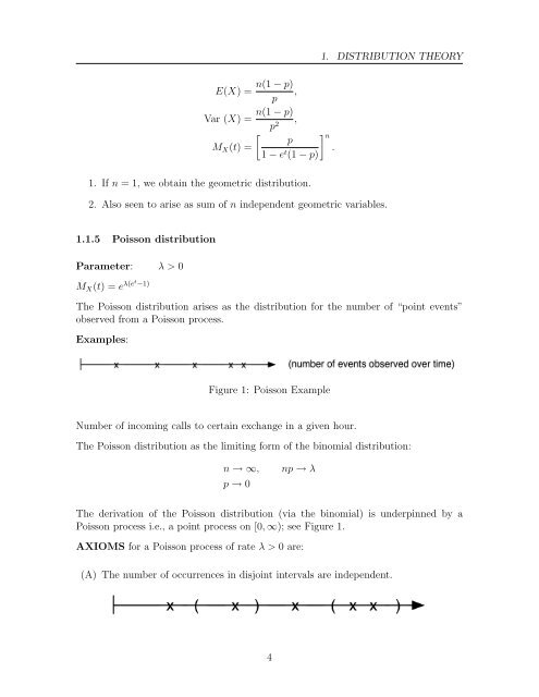
Examples:
Figure 1: Poisson Example
Number of incoming calls to certain exchange in a given hour.
The Poisson distribution as the limiting form of the binomial distribution:
n → ∞,
p → 0
np → λ
The derivation of the Poisson distribution (via the binomial) is underpinned by a
Poisson process i.e., a point process on [0, ∞); see Figure 1.
AXIOMS for a Poisson process of rate λ > 0 are:
(A) The number of occurrences in disjoint intervals are independent.
4