Seminar on Randomized Algorithms Game-Theoretical Applications ...

<strong>Seminar</strong> on Randomized Algorithms
Game-Theoretical Applications Part III
By Ibraguim Kouliev
In the following discussion we explore techniques for finding lower bounds for running
times of randomized game tree algorithms, and also address the general issues of
randomization and non-uniformity in algorithms.
Lower Bounds
First, we’ll discuss a method for obtaining lowest possible bounds for randomized game
tree evaluation algorithms.
A randomized game tree evaluation algorithm can be viewed as a probability distribution
over deterministic game-tree algorithms applied to random game tree instances. Thus,
we can use Yao’s Minimax principle for our task.
The Yao’s Minimax principle is essentially based on the following observation:
To find the lower bound for a randomized algorithm, it is sufficient to specify a
probability distribution on its input data and then prove a lower bound on the expected
running time of any deterministic algorithm operating on these data.
(One should note that this statement holds ONLY for Las Vegas algorithms!)
In our case, this means specifying a probability distribution on the values of the leaves of
a game tree and then finding the lower bound for any deterministic game-tree evaluation
algorithm applied to this tree.
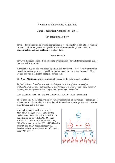
Although we could work with general
MIN-MAX trees, in order to simplify the
mathematics of our discussion we will focus
our attention on so-called AND-OR trees.
An AND-OR tree is a special type of binary
MIN-MAX tree, where [AND] and [OR] nodes
are MIN and MAX nodes, respectively.
Possible values for tree leaves are, of course,
binary “0” or “1”.

The first step is a simple modification of an AND-OR tree, which replaces all [AND] and
[OR] nodes by equivalent elements composed of [NOR] nodes (i.e. an [OR] is a negated
[NOR] etc).
This yields a NOR tree (which has the same depth due to redundancy of some of the
inner nodes). Though identical in terms of functionality, it also possesses a completely
homogenous structure, which further facilitates our calculations.
Second, we need to specify a probability distribution on values of the leaves. Each leaf is
independently set to “1”, with the following probability:
3−
p =
2
5
(Note: our peculiar choice of p will be justified by the next equation.)
The probability of a [NOR] node’s output being “1” is the probability that both inputs are
“0”, i.e.:
⎛ 2 3 − 5 ⎞ ⎛ 2 − 3 − 5 ⎞ ⎛ 5 −1⎞
3 − 5
(1 − p )(1 − p)
= ⎜ ⎟ ⎜ ⎟ = ⎜ ⎟
−
*
= =
⎝ 2 2 ⎠ ⎝ 2 ⎠ ⎝ 2 ⎠ 2
2
p
Now we consider some properties of a deterministic algorithm evaluating our tree. Since
we would like to minimize its running time, we make use of the following observation:

For a [NOR] node, the output value will be “0” if one of its
children returns “1”. In such cases, the other child (possibly
an entire sub-tree) will not influence the result, and
therefore, doesn’t need to be inspected.
This leads to a notion of Depth-First Pruning algorithms
(DFPA). A DFPA essentially functions like a DFS, but it
also stops visiting sub-trees of a node once its value has
been determined – sub-trees that yield no additional
information are “pruned” away.
Observe the following proposition:
Let T be a NOR tree, with all leaves set to the aforementioned distribution. Let W (T )
denote a minimum, over all deterministic game tree algorithms, of the expected number
of steps to evaluate T. Then, there exists a DFP algorithm, whose expected number of
steps to evaluate T is W (T ) .
Thus, for the purposes of our discussion, we may restrict ourselves to DFPAs.
For a DFPA, traversing a NOR tree with n leaves and aforementioned probability
distribution, the following holds:
Let h be the distance from the leaves to the node in
question. Let W (h)
denote the expected number of
leaves the DFPA will need to inspect in order to
evaluate the node.
Then:
W ( h)
= W ( h −1)
+ (1 − p)
⋅W
( h −1)
Here W ( h −1)
is the expected number of leaves visited
while evaluating one of the sub-trees of the node. The
factor ( 1− p)
before the second term arises from the
fact that the other sub-tree will only be visited if the
first sub-tree yielded 0, which will happen with the
probability of ( 1− p)
.
(Note: there is no factor p before the first term, as one might expect, because one of the
sub-trees must be visited under all circumstances, i.e. with 100 percent probability.)
Now we let h = log 2 n (since we are working with a binary tree), and substitute it into the
above equation. The solution of this equation produces the following result:
W ( h)
≥ n
0.694

We have thereby proven the following theorem:
The expected running time of any randomized algorithm that always evaluates an
instance of a binary MIN-MAX tree correctly is at least n 0.694 , where n=2 k is the number
of leaves.
Our result is slightly less than the bound of n 0.793 presented in the previous discussion by
Alexander Hombach. However, our method is correct (since it is based on Yao’s
Technique). One possibility is that our distribution of input values is not optimal, since it
does not preclude the possibility of both inputs to a NOR node being “1”. A distribution
that prevents such a possibility would show that the evaluation algorithm introduced in
the previous presentation is indeed optimal.
Randomness and Non-Uniformity
In the second part of our discussion, we try to answer the following question:
When is it possible to remove randomization from a randomized algorithm
For our analysis we need to introduce the notion of a randomized circuit. First, we give
the definition of a Boolean circuit:
A Boolean circuit with n inputs is a DAG with
following properties:
- It has n input vertices of in-degree 0, labeled
x x ,......
1
,
2
x n
- It has one output vertex of out-degree 0.
- Every inner vertex is labeled with a Boolean
function from the set [AND, OR, NOT]. A
vertex labeled [NOT] has in-degree 1.
- Every input can be assigned either 0 or 1.
- The output is a Boolean function of x
1
, x2,......
xn
. The circuit is said to compute this
function.
- The size of the circuit is the number of vertices in it.

A randomized circuit is very similar to a
Boolean circuit in terms of vertex properties, but
in addition to n circuit inputs it also has several
random inputs, labeled r 1
, r 2
,...... rn
. It computes
a function of x
1
, x2,......
xn
if following
conditions hold:
- For all x
1
, x2,......
xn
with f ( x 1
,...., x n
) = 0 the
output of the circuit is 0, regardless of the values
of random inputs.
- If f ( x 1
,...., x n
) = 1, the output is 1 with a
1
probability p ≥ .
2
Now consider a Boolean function f :{0,1}
∗ → {0,1 }.
n
Let fn
denote the function f restricted to inputs from { 0,1} . A sequence C = C 1, C 2,...
is
called a circuit family for f if Cn
has n inputs and computes f n
( x 1
,...., x n
) for all n-bit
inputs ( x
1
, x2,......
xn)
. The family C is polynomial-sized if the size of C
n
is bounded by a
polynomial in n for ∀ n .
A randomized circuit family for f is a family of randomized circuits, which has m
random inputs r , r ,...... r
1 2 m
in addition to inputs x
1
, x2,......
xn
, with r , r ,...... r
1 2 m
being
either 0 or 1 with equal probability. The properties of the circuits concerning random
inputs are those defined above.
All m-tuples ( r , r 1 2,......
r m)
, for which f ( ,...., )
n
x1 x n
= 1 for a particular n-tuple
( x
1
, x2,......
xn)
, are referred to as “witnesses” - they “testify” to the correct value of
f ( x 1
,...., ) = 1.
n
x n
We now introduce Adleman’s Theorem:
If a Boolean function has a randomized, polynomial-sized circuit family, then it has a
polynomial-sized circuit family.
As a proof we provide a method that removes randomization from a randomized
polynomial-sized circuit Cn
for fn( x1,....,
xn,
r1
,.... rm
) and transforms it into a deterministic
polynomial-sized circuit D that computes f x ,...., x ) :
n
n
( 1 n

n
n
First, we construct a matrix M with 2 rows for each possible n-tuple from { 0,1} and
m
m
2 columns for each possible random m-tuple from { 0,1} . An entry M
ij is 1 if the
corresponding m-tuple is witness for ( x 1
,...., x n
) , and 0 otherwise. Next, we eliminate all
rows for which f evaluates to 0, as there are no witnesses for such inputs.
We start the construction of our circuit by finding a column in which at least half the
entries are 1, that is, fn( x1 ,...., xn,
r1
,.... rm
) = 1for at least half the possible inputs
( x 1
,...., x n
) .
We then construct a circuit T1
as a copy of Cn
with random inputs “hard-wired” to the
values of the selected m-tuple (note that such a circuit is purely deterministic!), and
decimate the matrix by eliminating the selected column and all the rows that had 1’s in it.

Now we proceed in a similar fashion by selecting another column etc., until there are no
more rows left. As a result, we will have constructed at most n circuits T
1
, T2
,.... Tn
, which
we then combine into the final deterministic Boolean circuit, whose size is ( n +1)
times
the size of the original randomized circuit.
Our method is an example of a derandomization technique. Derandomization often
proves useful in design of deterministic algorithms – sometimes it is easier to devise a
randomized algorithm as a solution to some problem, and then derandomize it to arrive at
a deterministic algorithm. Unfortunately, it is not always possible or feasible to remove
randomization from polynomial-time computations, due to the issue of non-uniformity in
algorithms.

For further discussion we need to know what can be considered a non-uniform
(or a uniform) algorithm:
Let L denote a language over an alphabet ∑ * *
, and a : IN → ∑ , n → a(
n)
be a
mapping from positive integers to strings in L . An algorithm A is said to use the advice
a if on an input of length n it is given a string a (n)
on a read-only tape.
A decides L with a if on an input x it uses a ( x ) to decide x ∈ L . In other words, a
single a (n)
enables A to decide whether or not x ∈ L for ∀ x , x = n .
A uniform algorithm is an algorithm that doesn’t use such advice strings at all.
A non-uniform algorithm utilizes such advice strings.
For the complexity class P we define the class P / poly as a class of all languages L
that have a non-uniform polynomial-time algorithm A , such that length of all advice
strings a (n)
is polynomial-bounded in n , i.e. a ( n)
= O(
poly(
n))
. Likewise, we may
define the class RP / poly .
As an example, imagine a non-uniform algorithm A that processes words
*
{ x ∈∑ , x = n}
. Let a(n)
contain all { x ∈ L,
x = n}
. L would be in P / poly if the total
number of words in L were bounded by poly (n)
.
Similarly, we may speak of a language L as having a randomized circuit family. Then,
L ∈ RP / poly if and only if it has a randomized polynomial-sized circuit family.
Hence, one may interpret Adleman’s Theorem as a proof that
RP / poly ⊆ P /
poly
However, this only shows that removal of randomization can be done in principle. There
exist no uniform or practical methods for achieving this.
SUMMARY
In this discussion, we have covered the topics of randomized game tree algorithms,
Minimax Principle and Von Neumann’s Theorem, as well as Yao’s Techinques as
powerful tools for bound estimation. We also presented a method for evaluating the
lowest possible bound for a randomized algorithm, and addressed the issues of
randomization removal and non-uniformity in algorithms.
Bibliography:
Randomized Algorithms” by Rajeev Motwani and Prabhakar Raghavan
Cambridge University Press, 1995