Comprehensive approaches to 3D inversion of magnetic ... - CGISS

More documents

Recommendations

Info

L4 Li et al. the validity of the two-step approach. It is also noteworthy, however, that the estimation methods all rely on the global property of the magnetic data set. The estimated direction effectively summarizes the bulk direction of the magnetization in the causative bodies. The validity of the estimated direction relies on the assumption that actual direction does not vary significantly. In practice, the applicability of the approach is therefore limited to anomalies produced by single a) sources of compact geometry. For more complex scenarios, and when the magnetization direction is expected to vary greatly within the region of interest, an alternative approach is needed. 1000 800 B x Depth (m) 400 200 0 1000 Northing (m) 600 400 200 b) Northing (m) c) Northing (m) 800 600 400 200 Northing (m) 1000 800 600 400 200 0 1000 800 600 400 0 0 200 400 600 800 1000 Easting (m) 0 200 400 600 800 1000 T (nT) 450 400 350 300 250 200 150 100 50 0 50 100 150 Northing (m) Northing (m) 0 1000 800 600 400 200 0 1000 800 600 400 0 200 400 600 800 1000 250 B y 200 150 100 50 0 50 100 150 200 250 300 350 0 200 400 600 800 1000 B (nT) B z 200 200 0 0 200 400 600 800 1000 Easting (m) 0 0 200 400 600 800 1000 Easting (m) 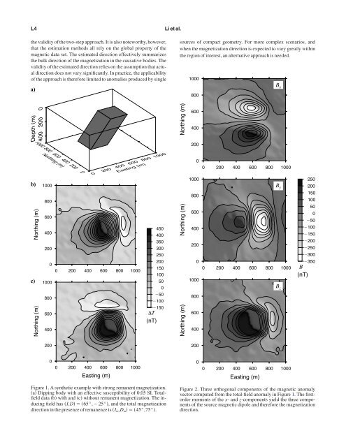Figure 1. A synthetic example with strong remanent magnetization. a Dipping body with an effective susceptibility of 0.05 SI. Totalfield data b with and c without remanent magnetization. The inducing field has I,D65°,25°, and the total magnetization direction in the presence of remanence is I m ,D m 45°,75°. Figure 2. Three orthogonal components of the magnetic anomaly vector computed from the total-field anomaly in Figure 1. The firstorder moments of the x- and z-components yield the three components of the source magnetic dipole and therefore the magnetization direction.
Magnetic inversion with remanence L5 INVERSION OF DATA WEAKLY DEPENDENT ON MAGNETIZATION DIRECTION Integrated mag (nT) Integrated mag (nT) 3000 2000 1000 0 1000 2000 0 200 400 600 800 1000 Easting (m) 3000 2000 1000 0 1000 2000 0 200 400 600 800 1000 Northing (m) Figure 3. Two synthesized profiles obtained from the data map shown in Figure 1b. The east-west profile top is obtained by integrating the map in the north-south direction; hence, it corresponds to the anomaly produced by a 2D causative body with a north-south strike. The north-south profile in the lower panel is obtained by integration in the east-west direction and corresponds to a 2D body with a strike in that direction. These profiles are used in wavelet estimation of the total magnetization direction. Inclination ( o ) 90 75 60 45 0.4 0.42 0.46 0.44 0.48 0.5 0.6 0.52 30 1801501209060 30 0 30 60 90 120 150 180 Declination ( o ) Figure 4. Crosscorrelation map between the total gradient of and vertical gradient of the RTP field computed from assumed inclination and declination of the magnetization. The crosscorrelation achieves maximum near the correct magnetization direction. 0.58 0.54 0.56 We now examine the more complex scenarios where a single estimated magnetization direction is no longer applicable. Such cases may arise if a geologic unit has undergone deformation because of tectonic activities so that the magnetization direction changes significantly within the source bodies, or when multiple source bodies acquire remanent magnetization at different times and have significantly different magnetization directions. The challenge faced in this case requires a completely new approach that does not rely on knowledge of magnetization direction. The inversion of data associated with magnetic anomalies but weakly dependent upon magnetization direction offers the needed alternative. The amplitude of the anomalous magnetic field vector and the total gradient of the magnetic anomaly are independent of the magnetization direction in 2D problems Nabighian, 1972 because the amplitude of the magnetic anomaly vector is the envelope of each component of the vector. The same holds true for the amplitude of the gradient vector of a 2D field component and the derivative of the same field component in any direction. Although such a property does not extend exactly to 3D problems, both quantities are only weakly dependent on magnetization direction. This is especially so when the anomaly has been transformed to the vertical component i.e., half RTP. This property provides the opportunity for direct inversion of the anomaly amplitude or total gradient to recover the magnitude of magnetization without knowing its direction. Shearer and Li 2004 develop such an algorithm by formulating a generalized inversion using Tikhonov regularization and imposing a Table 1. Magnetization direction estimated using three different methods for the dipping-slab data set shown in Figure 1c. The deviation is defined as the angle between the true and estimated directions in three dimensions. Method Inclination ° Declination ° Deviation ° True value 45 75 Helbig’s method 46 61 9.8 Wavelet method 49 68 6.2 Crosscorrelation 45 80 3.5 a) Depth (m) b) Northing (m) 0 200 400 1000 800 600 400 200 0 0 200 400 600 800 1000 0 200 400 600 800 1000 Easting (m) k (SI) 0.070 0.063 0.056 0.049 0.042 0.035 0.028 0.021 0.014 0.007 0.000 Figure 5. Effective susceptibility obtained through the inversion of the synthetic data in Figure 1b with estimated direction of total magnetization from Helbig’s method shown in Table 1. The inversion is performed using the algorithm of Li and Oldenburg 1996. a Cross section at 500 m north. b Plan section at a depth of 125 m. The true position of the source body is shown by the black outline. The resultant model is a good representation of the true model. The peak value of effective susceptibility is consistent with the true value of 0.05 SI.
Page 1 and 2: GEOPHYSICS, VOL. 75, NO. 1 JANUARY-
Page 3: Magnetic inversion with remanence L
Page 7 and 8: Magnetic inversion with remanence L
Page 9 and 10: Magnetic inversion with remanence L
Page 11: Magnetic inversion with remanence L

Comprehensive approaches to 3D inversion of magnetic ... - CGISS

You also want an ePaper? Increase the reach of your titles

Delete template?

Save as template?