Comprehensive approaches to 3D inversion of magnetic ... - CGISS

More documents

Recommendations

Info

L6 positivity constraint on the amplitude of magnetization. Shearer 2005 carries out a detailed investigation of the approach and demonstrates that the amplitude data are far less dependent on magnetization direction than the total gradient data. Furthermore, the amplitude data preserve the low-wavenumber content in the data and therefore retain the signal from deeper causative bodies that is present in the total-field magnetic anomaly. Consequently, inversion of amplitude data offers a better alternative than does inversion of total gradient data. We describe the amplitude inversion below, but readers are referred to Shearer 2005 for more details. The inversion of total gradient data is exactly parallel. Basic algorithm for amplitude inversion The algorithm starts by calculating the amplitude of the anomalous magnetic field from the observed total-field anomaly. This is accomplished by first transforming the total-field anomaly into the three orthogonal components in the x-, y-, and z-directions. The amplitude data are given by B a B a Bx 2 B y 2 B z 2 , where B a are the amplitude and B x ,B y ,B z are the transformed magnetic anomaly vectors. A common approach to obtain the three orthogonal components is to use the wavenumber-domain expressions e.g., Pedersen, 1978 when the data are located on a plane. Alternatively, equivalent-source techniques Dampney, 1969 can be used to carry out the transformation when ground data are acquired in areas with high topographic relief. In such cases, the wavenumber-domain approach, which assumes that all observations lie on a planar surface, is inappropriate. The amplitude data are then treated as the input data and inverted to recover the distribution of magnetization as a function of 3D position in the subsurface. One advantage of the approach is that it is not limited to a single anomaly nor does it require that adjacent anomalies have the same magnetization direction. Therefore, the approach is generally applicable to a wide range of problems where the source distribution is more complicated. The basic inversion algorithm follows that of Li and Oldenburg 1996, 2003 in which the Tikhonov formalism is used to trade off between the data misfit and the structural complexity of the recovered model. The data misfit is defined as N d i1 B obs pre ai B ai i 3 2 , 4 where B obs ai and B pre ai are observed and predicted amplitude data, respectively, and i are the standard deviation of the amplitude data. Although we commonly assume a Gaussian distribution for errors in magnetic field component data, the corresponding errors in the computed amplitude data no longer follow such a distribution. The model objective function is chosen as m s w 2 z 0 2 dv V wz 0 x V y V x wz 0 y 2 dv 2 dv Li et al. z V wz 0 z 2 dv, where is the effective susceptibility, defined as the ratio of magnitude of magnetization over the strength of the inducing field H 0 , 0 is a reference model, and wz is a depth-weighting function. The inverse solution is given by the minimization of the total objective function, consisting of a weighted sum of d and m , subject to the constraint that the effective susceptibility must be nonnegative: 5 minimize d m subject to 0, 6 where is the regularization parameter. The positivity is implemented by using a primal logarithmic barrier method Wright, 1997; Li and Oldenburg, 2003. The solution is obtained iteratively because nonlinearity is introduced by the positivity constraint and the nonlinear relationship between amplitude data and effective susceptibility. We discuss the basics of this aspect next, but readers are referred to Shearer 2005 for more details. We adopt a commonly used model representation that discretizes the model region in three dimensions into a set of contiguous rectangular prisms by an orthogonal mesh, and we assume a constant effective susceptibility value within each prism. Under this assumption, each component of the magnetic anomaly vector is given by a matrix-vector product: d x G x , d y G y , d z G z , where d x B x1 ,¯,B xN T is an algebraic vector holding the x-components of the anomalous magnetic field; d y and d z are similarly defined; 1 ,¯, M T is the vector of unknown effective susceptibility to be recovered; and G x , G y , and G z are the sensitivity matrices relating the respective components of anomalous magnetic field to effective susceptibilities. The elements of the sensitivity matrices quantify the field produced at the ith observation location by a unit effective susceptibility in the jth prism. Assuming the susceptibility model is n at the nth iteration, substituting equation 7 into equation 3 and differentiating B ai with respect to j yields n B ai B ai n j ·b ij, B ai where B n ai is the predicted anomalous magnetic vector at the ith observation location by the model n at the nth iteration and where b ij is the magnetic vector produced at the same location by a unit susceptibility in the jth prisms. Thus, the sensitivity has a simple and elegant form given by the inner product of the unit vector of the predicted magnetic field at the nth iteration and the magnetic field produced by a unit effective susceptibility in a prism. For computational purposes, this means we only need to compute and store the three sensitivity matrices corresponding to the three components of the field in equation 7 and calculate the sensitivity for the amplitude data by a sequence of matrix-vector multiplications when solving the minimization in equation 6. When calculating the three individual sensitivity matrices, we 7 8
Magnetic inversion with remanence L7 must formally specify a magnetization direction. Given that we are utilizing the weak dependence of amplitude data on magnetization direction, it is sufficient to use the direction of the current-inducing field. Thus, the sensitivity is computed as if the magnetization vector were given by the product of the effective susceptibility and the inducing field. It is important to note, however, that the interpretation of the inversion result is independent of the direction of the inducing field. The strength of the inducing field, on the other hand, defines the magnitude of the total magnetization if desired. Revisiting the synthetic example We now return to the synthetic example shown in Figure 1 and illustrate the approach of amplitude-data inversion. 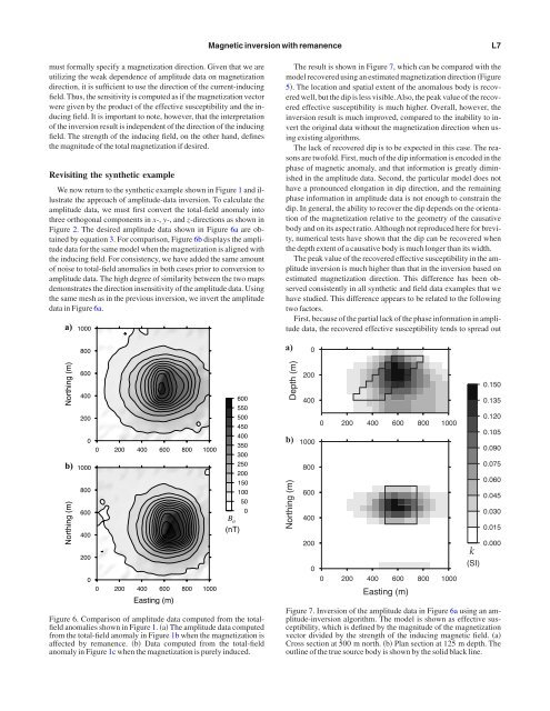To calculate the amplitude data, we must first convert the total-field anomaly into three orthogonal components in x-, y-, and z-directions as shown in Figure 2. The desired amplitude data shown in Figure 6a are obtained by equation 3. For comparison, Figure 6b displays the amplitude data for the same model when the magnetization is aligned with the inducing field. For consistency, we have added the same amount of noise to total-field anomalies in both cases prior to conversion to amplitude data. The high degree of similarity between the two maps demonstrates the direction insensitivity of the amplitude data. Using the same mesh as in the previous inversion, we invert the amplitude data in Figure 6a. a) 1000 The result is shown in Figure 7, which can be compared with the model recovered using an estimated magnetization direction Figure 5. The location and spatial extent of the anomalous body is recovered well, but the dip is less visible.Also, the peak value of the recovered effective susceptibility is much higher. Overall, however, the inversion result is much improved, compared to the inability to invert the original data without the magnetization direction when using existing algorithms. The lack of recovered dip is to be expected in this case. The reasons are twofold. First, much of the dip information is encoded in the phase of magnetic anomaly, and that information is greatly diminished in the amplitude data. Second, the particular model does not have a pronounced elongation in dip direction, and the remaining phase information in amplitude data is not enough to constrain the dip. In general, the ability to recover the dip depends on the orientation of the magnetization relative to the geometry of the causative body and on its aspect ratio.Although not reproduced here for brevity, numerical tests have shown that the dip can be recovered when the depth extent of a causative body is much longer than its width. The peak value of the recovered effective susceptibility in the amplitude inversion is much higher than that in the inversion based on estimated magnetization direction. This difference has been observed consistently in all synthetic and field data examples that we have studied. This difference appears to be related to the following two factors. First, because of the partial lack of the phase information in amplitude data, the recovered effective susceptibility tends to spread out 800 a) 0 Northing (m) b) Northing (m) 600 400 200 0 1000 800 600 400 200 0 0 200 400 600 800 1000 0 200 400 600 800 1000 Easting (m) B a (nT) Figure 6. Comparison of amplitude data computed from the totalfield anomalies shown in Figure 1. a The amplitude data computed from the total-field anomaly in Figure 1b when the magnetization is affected by remanence. b Data computed from the total-field anomaly in Figure 1c when the magnetization is purely induced. 600 550 500 450 400 350 300 250 200 150 100 50 0 Depth (m) b) Northing (m) 200 400 1000 800 600 400 200 0 0 200 400 600 800 1000 0 200 400 600 800 1000 Easting (m) k (SI) 0.150 0.135 0.120 0.105 0.090 0.075 0.060 0.045 0.030 0.015 0.000 Figure 7. Inversion of the amplitude data in Figure 6a using an amplitude-inversion algorithm. The model is shown as effective susceptibility, which is defined by the magnitude of the magnetization vector divided by the strength of the inducing magnetic field. a Cross section at 500 m north. b Plan section at 125 m depth. The outline of the true source body is shown by the solid black line.
Page 1 and 2: GEOPHYSICS, VOL. 75, NO. 1 JANUARY-
Page 3 and 4: Magnetic inversion with remanence L
Page 5: Magnetic inversion with remanence L
Page 9 and 10: Magnetic inversion with remanence L
Page 11: Magnetic inversion with remanence L

Comprehensive approaches to 3D inversion of magnetic ... - CGISS

You also want an ePaper? Increase the reach of your titles

Delete template?

Save as template?