Comprehensive approaches to 3D inversion of magnetic ... - CGISS

L6
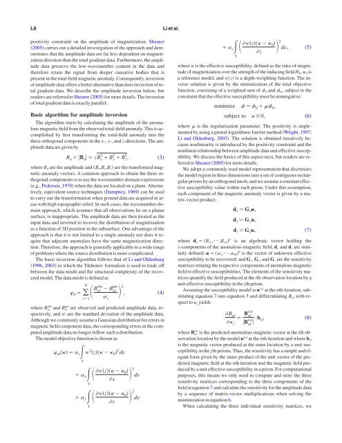
positivity constraint on the amplitude of magnetization. Shearer
2005 carries out a detailed investigation of the approach and demonstrates
that the amplitude data are far less dependent on magnetization
direction than the total gradient data. Furthermore, the amplitude
data preserve the low-wavenumber content in the data and
therefore retain the signal from deeper causative bodies that is
present in the total-field magnetic anomaly. Consequently, inversion
of amplitude data offers a better alternative than does inversion of total
gradient data. We describe the amplitude inversion below, but
readers are referred to Shearer 2005 for more details. The inversion
of total gradient data is exactly parallel.
Basic algorithm for amplitude inversion
The algorithm starts by calculating the amplitude of the anomalous
magnetic field from the observed total-field anomaly. This is accomplished
by first transforming the total-field anomaly into the
three orthogonal components in the x-, y-, and z-directions. The amplitude
data are given by
B a B a Bx 2 B y 2 B z 2 ,
where B a are the amplitude and B x ,B y ,B z are the transformed magnetic
anomaly vectors. A common approach to obtain the three orthogonal
components is to use the wavenumber-domain expressions
e.g., Pedersen, 1978 when the data are located on a plane. Alternatively,
equivalent-source techniques Dampney, 1969 can be used
to carry out the transformation when ground data are acquired in areas
with high topographic relief. In such cases, the wavenumber-domain
approach, which assumes that all observations lie on a planar
surface, is inappropriate. The amplitude data are then treated as the
input data and inverted to recover the distribution of magnetization
as a function of 3D position in the subsurface. One advantage of the
approach is that it is not limited to a single anomaly nor does it require
that adjacent anomalies have the same magnetization direction.
Therefore, the approach is generally applicable to a wide range
of problems where the source distribution is more complicated.
The basic inversion algorithm follows that of Li and Oldenburg
1996, 2003 in which the Tikhonov formalism is used to trade off
between the data misfit and the structural complexity of the recovered
model. The data misfit is defined as
N
d
i1
B obs pre
ai B ai
i
3
2
, 4
where B obs ai and B pre ai are observed and predicted amplitude data, respectively,
and i are the standard deviation of the amplitude data.
Although we commonly assume a Gaussian distribution for errors in
magnetic field component data, the corresponding errors in the computed
amplitude data no longer follow such a distribution.
The model objective function is chosen as
m s w 2 z 0 2 dv
V
wz 0
x
V
y
V
x
wz 0
y
2
dv
2
dv
Li et al.
z V
wz 0
z
2
dv,
where is the effective susceptibility, defined as the ratio of magnitude
of magnetization over the strength of the inducing field H 0 , 0 is
a reference model, and wz is a depth-weighting function. The inverse
solution is given by the minimization of the total objective
function, consisting of a weighted sum of d and m , subject to the
constraint that the effective susceptibility must be nonnegative:
5
minimize d m
subject to 0, 6
where is the regularization parameter. The positivity is implemented
by using a primal logarithmic barrier method Wright, 1997;
Li and Oldenburg, 2003. The solution is obtained iteratively because
nonlinearity is introduced by the positivity constraint and the
nonlinear relationship between amplitude data and effective susceptibility.
We discuss the basics of this aspect next, but readers are referred
to Shearer 2005 for more details.
We adopt a commonly used model representation that discretizes
the model region in three dimensions into a set of contiguous rectangular
prisms by an orthogonal mesh, and we assume a constant effective
susceptibility value within each prism. Under this assumption,
each component of the magnetic anomaly vector is given by a matrix-vector
product:
d x G x ,
d y G y ,
d z G z ,
where d x B x1 ,¯,B xN T is an algebraic vector holding the
x-components of the anomalous magnetic field; d y and d z are similarly
defined; 1 ,¯, M T is the vector of unknown effective
susceptibility to be recovered; and G x , G y , and G z are the sensitivity
matrices relating the respective components of anomalous magnetic
field to effective susceptibilities. The elements of the sensitivity matrices
quantify the field produced at the ith observation location by a
unit effective susceptibility in the jth prism.
Assuming the susceptibility model is n at the nth iteration, substituting
equation 7 into equation 3 and differentiating B ai with respect
to j yields
n
B ai
B ai
n j ·b ij,
B ai
where B n ai is the predicted anomalous magnetic vector at the ith observation
location by the model n at the nth iteration and where b ij
is the magnetic vector produced at the same location by a unit susceptibility
in the jth prisms. Thus, the sensitivity has a simple and elegant
form given by the inner product of the unit vector of the predicted
magnetic field at the nth iteration and the magnetic field produced
by a unit effective susceptibility in a prism. For computational
purposes, this means we only need to compute and store the three
sensitivity matrices corresponding to the three components of the
field in equation 7 and calculate the sensitivity for the amplitude data
by a sequence of matrix-vector multiplications when solving the
minimization in equation 6.
When calculating the three individual sensitivity matrices, we
7
8