Comprehensive approaches to 3D inversion of magnetic ... - CGISS

More documents

Recommendations

Info

L8 Li et al. more. There is essentially more susceptibility distributed at larger depth. Correspondingly, a higher peak value is required to reproduce the data. For example, the depths of the center of mass of the susceptibility are 200 and 280 m, respectively, in the models from inversion using estimated direction Figure 5 and from amplitude inversion Figure 7. The cube of the ratio of the two depths is 0.35. Given that the amplitude data decay approximately with inverse distance cubed, this ratio is consistent with the peak susceptibility ratio of 0.45. Second, every small anomalous feature in the amplitude data can be reproduced easily, so the data tend to be overfit when we use standard techniques for estimating the optimal data fit determined by the regularization parameter. This also leads to a greater peak susceptibility value in recovered models. However, the geometry of the recovered source body is similar for the two inversions despite the difference in peak susceptibility values. Both models can be used to carry out the final interpretation. The ability to invert amplitude data has effectively circumvented the need for magnetization direction as a crucial piece of information. As a result, we have bypassed the limitation of the first method that requires a constant magnetization direction within a source body. This opens the door to applying 3D inversion to interpret a wide range of data sets, especially those from areas with complex geology and multiple source regions with variable magnetization directions. APPLICATION TO FIELD DATA SETS We now invert two sets of high-resolution aeromagnetic data and illustrate the application of our methods in their respective scenarios. The data were acquired by TeckCominco and Diamonds North over kimberlites on Victoria Island in Northwest Territory, Canada. The geology in the area is characterized by an Archean granitic basement overlain by a Proterozoic sedimentary sequence with minor volcanics, capped by flat-lying Cambrian-to-Devonian carbonate rocks. The host rocks are largely nonmagnetic, and the kimberlite bodies stand out in the magnetic surveys as distinct, sharp anomalies indicative of shallow bodies, compared with the more rounded anomalies caused by deep features in the basement or within the sedimentary rocks. Positive and negative anomalies are associated with kimberlite intrusions, whereas the negative anomalies are produced by hypabyssal dikes. The ages of the kimberlite intrusions range from 250 to 300 million years J. Lajoie, personal communication, 2004. The distinct magnetic signature of these kimberlite dikes above a quiet magnetic background makes high-resolution magnetic surveys an ideal exploration tool in this area. However, the highly variable orientation of these anomalies is produced by magnetization that is dominated by strong remanence with variable direction. As a result, the quantitative interpretation of the anomalies is difficult to achieve through current 3D inversion algorithms. For this reason, the data are ideal for testing our new approaches. We investigate data from two different areas with variable complexity in anomaly patterns. The first data set contains a single anomaly associated with a kimberlite dike; the second contains several different anomalies with large variations in magnetization direction. The data set containing a single anomaly is shown in Figure 8a. The inducing field has an inclination of 86.7° and declination of 26.3°. Given the high magnetic latitude and dominant negative anomaly, it is clear that the kimberlite has strong remanence, and the total magnetization is nearly in the opposite direction to the inducing field. Figure 8b displays the amplitude data computed from these data. Given the single anomaly in this data set, we can estimate the direction first and then invert the total-field data or we can directly invert the amplitude data. We present both for comparison. The results of estimation are listed in Table 2. The estimated values for inclination are similar, but the declination varies greatly. This is expected, given the inclination is close to 90°. When used in an inversion, the error in declination does not strongly affect the final result either. Using the direction estimated from multiscale edges, inversion of total-field data Figure 8a is shown in one cross section at 300 m north and one plan section at 50 m depth in Figure 9. The result from inverting the amplitude data is shown in the same format in Figure 10. The two inversions recover models with similar geometry but differing peak susceptibility, as noted in the preceding section. Both effectively image a compact magnetic body. It has a northwest strike and a strike length of approximately 250 m, and it is located at 50 m depth to the center. This result is consistent with the presence of a kimberlite dike. The second data set is shown in Figure 11a. A number of dipolar total-field anomalies with differing orientations occur throughout the survey area. The map has been rotated clockwise by 34°; the inducing field has an inclination of 86.7° and a nominal declination of 7.7°. Two types of anomalies dominate the data set: several smaller, more compact, and high-frequency anomalies surrounding areas a) Northing (m) b) Northing (m) 600 400 200 0 600 400 200 0 0 200 400 600 800 0 200 400 600 800 Easting (m) 4 3 2 1 0 1 2 3 4 5 6 7 8 T (nT) 7.0 6.5 6.0 5.5 5.0 4.5 4.0 3.5 3.0 2.5 2.0 1.5 1.0 0.5 0.0 B a (nT) Figure 8. a Total-field magnetic anomaly T over a kimberlite dike. The inducing field is in the direction of I86.7° and D 26.3°. Judging from the negative anomaly in the center, the presence of strong remanent magnetization is apparent. b The corresponding amplitude, B a , of the anomalous field vector.
Magnetic inversion with remanence L9 of broad, lower-frequency anomalies. The orientation of the anomalies indicates the total magnetization direction varies greatly from anomaly to anomaly. Thus, it is unlikely that we can invert this data set with a single magnetization direction. Overlapping anomalies also mean that separately inverting each anomaly by first estimating a magnetization direction is not feasible. We resort to the second approach, i.e., we invert the amplitude of the anomalous magnetic field and recover the magnitude of magnetization in the form of an effective susceptibility. The computed amplitude data are shown in Figure 11b. The effective susceptibility recovered from the inversion of the amplitude data in Figure 11b is shown in Figure 12 as a volume-rendered image with an overlain translucent color display of the amplitude data. There are five main anomalous bodies of high susceptibility in the recovered model. The two broad, elongated bodies resemble kimberlite dikes known in this area, whereas the more compact bodies oriented vertically resemble kimberlite pipes. DISCUSSION Table 2. Magnetization direction estimated using three different methods for the field data set shown in Figure 8a. Method Inclination ° Declination ° Helbig’s method 84.7 70.0 Wavelet method 89.3 1.8 Crosscorrelation 87.4 26.0 The methodology developed in this paper for inverting magnetic data in the presence of remanent magnetization consists of two approaches. The first approach directly addresses the issue of unknown magnetization direction and estimates it using several existing and newly developed algorithms. The data are then inverted using existing magnetic inversion algorithms. The second approach circumvents the need for reliable knowledge of magnetization direction and, instead, inverts directly the amplitude of the anomalous field to recover the magnitude of the magnetization. Figure 13 summarizes the three routes to the inversion of magnetic data. For a given data set, the first question to be answered is whether the data are affected by strong remanent magnetization that is not aligned with the current inducing field. If the answer is no, then any standard inversion algorithms for 3D magnetic inversion can be applied. If the answer is yes, the data set should be inverted by using one of two approaches depending on the complexity of the magnetic anomaly. The criterion for choosing which method to use is whether a single magnetization direction is a valid assumption and can be estimated. If the answer is yes, then the method based on direction estimation should be used. In practice, this means that only a single compact anomaly is present, although rare cases of multiple anomalies with the same magnetization direction may exist. If the answer is no, then the amplitude-data inversion method should be used. Such cases include a single anomaly produced by a complex source body or multiple anomalies with different orientations. Both methods can effectively construct the source distribution for a compact source body that meets the assumption of a constant magnetization direction. However, when multiple source bodies are present with varying magnetization directions, amplitude-data inversion proves to be much more versatile. 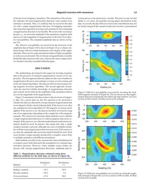The price we pay for that ability is, of course, the partially missing phase information in the data.As a result, the dip of the recovered source distribution may not be clearly imaged if the causative body does not have a pronounced a) Depth (m) b) Northing (m) 0 50 100 150 200 300 400 500 600 500 400 300 200 200 300 400 500 600 Easting (m) 1.0 0.9 0.8 0.7 0.6 0.5 0.4 0.3 0.2 0.1 0.0 k (SI) Figure 9. Effective susceptibility recovered by inverting the totalfield magnetic anomaly in Figure 8a. The inversion uses the magnetization direction estimated by the multiscale edge method. a Cross section at 300 m north. b Plan section at 50 m depth. a) Depth (m) b) Northing (m) 0 50 100 150 200 300 400 500 600 500 400 300 200 200 300 400 500 600 Easting (m) k (SI) 0.020 0.018 0.016 0.014 0.012 0.010 0.008 0.006 0.004 0.002 0.000 Figure 10. Effective susceptibility recovered by inverting the amplitude anomaly in Figure 8b. a Cross section at 300 m north. b Plan section at 50 m depth.
Page 1 and 2: GEOPHYSICS, VOL. 75, NO. 1 JANUARY-
Page 3 and 4: Magnetic inversion with remanence L
Page 5 and 6: Magnetic inversion with remanence L
Page 7: Magnetic inversion with remanence L
Page 11: Magnetic inversion with remanence L

Comprehensive approaches to 3D inversion of magnetic ... - CGISS

You also want an ePaper? Increase the reach of your titles

Delete template?

Save as template?