Selecting the Right Objective Measure for Association Analysis*

More documents

Recommendations

Info

Using Definition 1, we can determine the consistency between every pair of measures by computing the correlation between their ranking vectors. Figure 5 depicts the pair-wise correlation when various support bounds are imposed. We have re-ordered the correlation matrix using the reverse Cuthill-McKee algorithm [17] so that the darker cells are moved as close as possible to the main diagonal. The darker cells indicate that the correlation between the pair of measures is approximately greater than 0.8. Initially, without support pruning, we observe that many of the highly correlated measures agree with the seven groups of measures identified in Section 4.3. For Group 1 through Group 5, the pairwise correlations between measures from the same group are greater than 0.94. For Group 6, the correlation between interest factor and added value is 0.948; interest factor and K is 0.740; and K and added value is 0.873. For Group 7, the correlation between mutual information and κ is 0.936; mutual information and certainty factor is 0.790; and κ and certainty factor is 0.747. These results suggest that the properties defined in Table 6 may explain most of the high correlations in the upper left-hand diagram shown in Figure 5. Next, we examine the effect of applying a maximum support threshold to the contingency tables. The result is shown in the upper right-hand diagram. Notice the growing region of dark cells compared to the previous case, indicating that more measures are becoming highly correlated with each other. Without support-based pruning, nearly 40% of the pairs have correlation above 0.85. With maximum support pruning, this percentage increases to more than 68%. For example, interest factor, which is quite inconsistent with almost all other measures except for added value, have become more consistent when high-support items are removed. This observation can be explained as an artifact of interest factor. 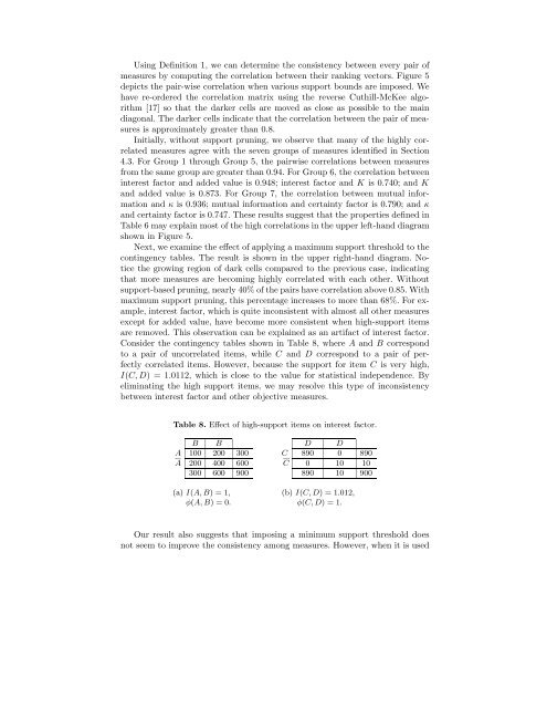Consider the contingency tables shown in Table 8, where A and B correspond to a pair of uncorrelated items, while C and D correspond to a pair of perfectly correlated items. However, because the support for item C is very high, I(C, D) = 1.0112, which is close to the value for statistical independence. By eliminating the high support items, we may resolve this type of inconsistency between interest factor and other objective measures. Table 8. Effect of high-support items on interest factor. B B D D A 100 200 300 C 890 0 890 A 200 400 600 C 0 10 10 300 600 900 890 10 900 (a) I(A, B) = 1, (b) I(C, D) = 1.012, φ(A, B) = 0. φ(C, D) = 1. Our result also suggests that imposing a minimum support threshold does not seem to improve the consistency among measures. However, when it is used
along with a maximum support threshold, the correlations among measures do show some slight improvements compared to applying the maximum support threshold alone — more than 71% of the pairs have correlation above 0.85. This analysis suggests that imposing a tighter bound on the support of association patterns may force many measures become highly correlated with each other. 6 Table Standardization Standardization is a widely-used technique in statistics, political science, and social science studies to handle contingency tables that have different marginals. Mosteller suggested that standardization is needed to get a better idea of the underlying association between variables [25], by transforming an existing table so that their marginals become equal, i.e., f ∗ 1+ = f ∗ 0+ = f ∗ +1 = f ∗ +0 = N/2 (see Table 9). A standardized table is useful because it provides a visual depiction of how the joint distribution of two variables would look like after eliminating biases due to non-uniform marginals. Table 9. Table Standardization. B B B B B B A f 11 f 10 f 1+ A f11 ∗ f10 ∗ f1+ ∗ A x N/2 − x N/2 A f 01 f 00 f 0+ −→ A f01 ∗ f00 ∗ f0+ ∗ −→ A N/2 − x x N/2 f +1 f +0 N f+1 ∗ f+0 ∗ N N/2 N/2 N 6.1 Effect of Non-Uniform Marginals Standardization is important because some measures can be affected by differences in the marginal totals. To illustrate this point, consider a pair of contingency tables, X = [a b; c d] and Y = [p q; r s]. We can compute the difference between the φ-coefficients for both tables as follows. log(φ X ) = log(ad − bc) − 1 [log(a + b) + log(a + c) 2 + log(b + c) + log(b + d)] (1) log(φ Y ) = log(pq − rs) − 1 [log(p + q) + log(p + r) 2 + log(q + s) + log(r + s)] (2) where the φ-coefficient is expressed as a logarithmic value to simplify the calculations. The difference between the two coefficients can be written as log(φ X ) − log(φ Y ) = ∆ 1 − 0.5∆ 2 ,
Page 1 and 2: Selecting the Right Objective Measu
Page 3 and 4: Table 3. Rankings of contingency ta
Page 5 and 6: Bayardo et al. [6] compared the opt
Page 7 and 8: goodness of fit testing, it is seld
Page 9 and 10: 4 Properties of Objective Measures
Page 11 and 12: B B A p q A r s A A B p r B q s (a)
Page 13 and 14: using φ-coefficient and other symm
Page 15 and 16: highly correlated patterns inadvert
Page 17: CF Conviction Yule Y Odds ratio Yul
Page 21 and 22: k=0 k=1 15 10 25 35 40 75 50 50 100
Page 23 and 24: 6.4 Generalized Standardization Pro
Page 25 and 26: Unfortunately, asking the experts t
Page 27 and 28: a All Contingency Tables B = 1 B =
Page 29 and 30: is quite consistent with the orderi
Page 31 and 32: 6. R. Bayardo and R. Agrawal. Minin

Selecting the Right Objective Measure for Association Analysis*

Create successful ePaper yourself

Delete template?

Save as template?