Flo-Tote 3 Sensor User Manual - Hachflow
Flo-Tote 3 Sensor User Manual - Hachflow
Flo-Tote 3 Sensor User Manual - Hachflow

Create successful ePaper yourself
Turn your PDF publications into a flip-book with our unique Google optimized e-Paper software.
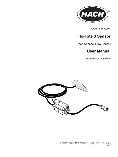
DOC026.53.00787<br />
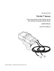
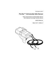
<strong>Flo</strong>-<strong>Tote</strong> 3 <strong>Sensor</strong><br />
Open Channel <strong>Flo</strong>w <strong>Sensor</strong><br />
<strong>User</strong> <strong>Manual</strong><br />
November 2013, Edition 4<br />
© Hach Company, 2010. All rights reserved. Printed in the U.S.A<br />
jk/kt
Table of Contents<br />
Section 1 Specifications.................................................................................................................... 3<br />
Section 2 General Information......................................................................................................... 5<br />
2.1 Safety information........................................................................................................................ 5<br />
2.1.1 Use of hazard information................................................................................................... 5<br />
2.1.2 Precautionary labels ........................................................................................................... 5<br />
2.1.3 Confined space entry .......................................................................................................... 6<br />
2.2 Product overview ......................................................................................................................... 6<br />
2.2.1 <strong>Flo</strong>-<strong>Tote</strong> 3 flow system features.......................................................................................... 6<br />
2.2.2 Applications of a <strong>Flo</strong>-<strong>Tote</strong> 3 system.................................................................................... 6<br />
2.2.3 Advantages of a <strong>Flo</strong>-<strong>Tote</strong> 3 system .................................................................................... 7<br />
2.3 Theory of operation...................................................................................................................... 7<br />
2.3.1 Velocity measurement ........................................................................................................ 7<br />
2.3.2 Depth measurement ........................................................................................................... 8<br />
2.3.3 <strong>Flo</strong>w calculation .................................................................................................................. 8<br />
Section 3 Installation.......................................................................................................................... 9<br />
3.1 Component list ............................................................................................................................. 9<br />
3.2 Site location guidelines ................................................................................................................ 9<br />
3.3 <strong>Sensor</strong> installation...................................................................................................................... 12<br />
3.3.1 <strong>Sensor</strong> installation kits ...................................................................................................... 12<br />
3.3.2 Connection to the <strong>Flo</strong>-Logger, FL900 Series Logger or <strong>Flo</strong>-Station ................................. 12<br />
3.4 Dams for low-flow applications .................................................................................................. 13<br />
3.4.1 Dam construction .............................................................................................................. 13<br />
3.4.2 Dam installation ................................................................................................................ 14<br />
Section 4 Maintenance .................................................................................................................... 15<br />
4.1 <strong>Sensor</strong> cleaning ......................................................................................................................... 15<br />
4.2 Changing the <strong>Sensor</strong> Desiccant ................................................................................................15<br />
4.2.1 Desiccant replacement procedure .................................................................................... 15<br />
4.3 Hydrophobic filter description..................................................................................................... 16<br />
4.4 Hydrophobic filter replacement procedure ................................................................................. 17<br />
Section 5 Troubleshooting ............................................................................................................. 19<br />
Section 6 Contact Information ....................................................................................................... 21<br />
Appendix A Velocity profiling ........................................................................................................ 23<br />
A.1 About velocity profiling............................................................................................................... 23<br />
A.2 Site selection ............................................................................................................................. 24<br />
A.3 Profile guidelines ....................................................................................................................... 24<br />
A.4 Depth of flow measurements..................................................................................................... 24<br />
A.5 Velocity profile calculations ....................................................................................................... 25<br />
A.5.1 .9 x Vmax method............................................................................................................. 25<br />
A.5.2 .2, .4, .8 method................................................................................................................ 26<br />
A.5.3 .4 method.......................................................................................................................... 26<br />
A.5.4 2D method ........................................................................................................................ 26<br />
A.6 Auto-Cal automatic calibration................................................................................................... 28<br />
A.7 Calibrate the sensor using the Cal Wizard in the <strong>Flo</strong>-Ware software ........................................ 28<br />
Appendix B <strong>Flo</strong>w calculations ....................................................................................................... 29<br />
B.1 Circular channels....................................................................................................................... 29<br />
B.2 Rectangular channels................................................................................................................ 32<br />
B.3 Rivers and streams.................................................................................................................... 33<br />
B.4 <strong>Flo</strong>w unit conversions................................................................................................................ 35<br />
1
Table of Contents<br />
2
Section 1<br />
Specifications<br />
Specifications are subject to change without notice.<br />
Table 1 <strong>Sensor</strong> specifications<br />
General<br />
Material<br />
Dimensions<br />
Weight<br />
Operating temperature<br />
Polyurethane<br />
13.1 cm W x 4.4 cm L x 2.8 cm diameter (5.16 in. x 1.73 in. x 1.10 in.)<br />
1.1 kg (2.4 lb) with 30 ft cable<br />
0 to 45 °C (32 to 113 °F)<br />
Operating humidity 0-100%<br />
Storage temperature –20 to 52° C (–4 to 125° F)<br />
Power requirements<br />
Velocity measurement<br />
Depth measurement<br />
<strong>Flo</strong>w measurement<br />
Temperature<br />
measurement<br />
<strong>Sensor</strong> cable<br />
Warranty<br />
Warranty<br />
10V, 100 mA. <strong>Sensor</strong> power is supplied by the portable <strong>Flo</strong>-Logger or by the <strong>Flo</strong>-Station<br />
Monitor.<br />
Method: Electromagnetic (Faraday’s law)<br />
Range: –1.5 to 6.1 m/s (–5 to 20 ft/s)<br />
Accuracy: ± 2% of reading<br />
Zero stability: ± 0.015 m/s (± 0.05 ft/s) at 0 to 3 m/s (0 to 10 ft/s)<br />
Resolution: ± 0.0003 m/s (0.01 ft/s)<br />
Method: Submerged pressure transducer<br />
Range: Standard 10 mm to 3.5 m (0.4 to 138 inches). Contact the factory for extended ranges<br />
Accuracy: ± 1% reading<br />
Zero stability: ± 0.009 m (± 0.03 feet), for 0 to 3 m (0 to 10 ft)<br />
Includes non-linearity, hysteresis and velocity effects.<br />
Resolution: 2.5 mm (0.1 in.)<br />
Over range protection: 2X range<br />
Method: Conversion of water level and pipe size to fluid area. Conversion of local velocity<br />
reading to mean velocity. Multiplication of fluid area by mean velocity to equal flow rate.<br />
Conversion accuracy: ± 5.0% of reading. Assumes appropriate site calibration coefficient, pipe<br />
flowing 10% to 90% full with a level greater than 5.08 cm (2 in.).<br />
Method: 1 wire digital thermometer<br />
Range: –10 to 85 °C (14 to 185 °F)<br />
Accuracy: ± 2 °C (± 3.5 °F)<br />
Material: Polyurethane jacketed<br />
Standard length: 9.1 m (30 ft)<br />
Optional length: 18.2 m, 30.4 m (60,100 ft) or length as needed; maximum 304 m (1000 ft)<br />
One year from date of shipment. Does not apply to such consumable components, such as,<br />
but not limited to, desiccants and batteries.<br />
3
Specifications<br />
4
Section 2<br />
General Information<br />
2.1 Safety information<br />
2.1.1 Use of hazard information<br />
2.1.2 Precautionary labels<br />
Please read this entire manual before unpacking, setting up or operating this equipment.<br />
Pay attention to all danger, warning and caution statements. Failure to do so could result<br />
in serious injury to the operator or damage to the equipment.<br />
Make sure that the protection provided by this equipment is not impaired, do not use or<br />
install this equipment in any manner other than that specified in this manual.<br />
DANGER<br />
Indicates a potentially or imminently hazardous situation which, if not avoided, will<br />
result in death or serious injury.<br />
WARNING<br />
Indicates a potentially or imminently hazardous situation which, if not avoided,<br />
could result in death or serious injury.<br />
CAUTION<br />
Indicates a potentially hazardous situation that may result in minor or moderate<br />
injury.<br />
Notice: Indicates a situation that is not related to personal injury.<br />
Important Note: Indicates a situation which, if not avoided, may cause damage to the<br />
instrument. Information that requires special emphasis.<br />
Note: Information that supplements points in the main text.<br />
Read all labels and tags attached to the instrument. Personal injury or damage to the<br />
instrument could occur if not observed. A symbol, if noted on the instrument, will be<br />
included with a danger or caution statement in the manual.<br />
This is the safety alert symbol. Obey all safety messages that follow this symbol to avoid potential injury. If on the<br />
instrument, refer to the instruction manual for operation or safety information.<br />
Electrical equipment marked with this symbol may not be disposed of in European public disposal systems after 12<br />
August of 2005. In conformity with European local and national regulations (EU Directive 2002/96/EC), European<br />
electrical equipment users must now return old or end-of life equipment to the Producer for disposal at no charge to<br />
the user.<br />
Note: For return for recycling, please contact the equipment producer or supplier for instructions on how to return<br />
end-of-life equipment, producer-supplied electrical accessories, and all auxiliary items for proper disposal.<br />
This symbol, when noted on the product, indicates the presence of devices sensitive to Electro-static Discharge<br />
(ESD) and indicates that care must be taken to prevent damage with the equipment.<br />
5
General Information<br />
2.1.3 Confined space entry<br />
2.2 Product overview<br />
The following information is provided to guide users of <strong>Flo</strong>-<strong>Tote</strong> 3 sensors on the dangers<br />
and risks associated with entry into confined spaces.<br />
WARNING<br />
Potential confined space hazards. Training in pre-entry testing, ventilation, entry<br />
procedures, evacuation/rescue procedures and safety work practices is necessary<br />
to ensure against the loss of life in confined spaces.<br />
On April 15, 1993, OSHA's final ruling on CFR 1910.146, Permit Required Confined<br />
Spaces, became law. This standard directly affects more than 250,000 industrial sites in<br />
the United States and was created to protect the health and safety of workers in confined<br />
spaces.<br />
Definition of Confined Space<br />
A Confined Space is any location or enclosure that presents or has the immediate<br />
potential to present one or more of the following conditions:<br />
• An atmosphere with less than 19.5% or greater than 23.5% oxygen and/or more than<br />
10 ppm Hydrogen Sulfide (H2S)<br />
• An atmosphere that may be flammable or explosive due to gases, vapors, mists,<br />
dusts, or fibers<br />
• Toxic materials which upon contact or inhalation, could result in injury, impairment of<br />
health, or death<br />
Confined spaces are not designed for human occupancy. They have restricted entry and<br />
contain known or potential hazards. Examples of confined spaces include manholes,<br />
stacks, pipes, vats, switch vaults, and other similar locations.<br />
Standard safety procedures must always be followed prior to entry into confined spaces<br />
and/or locations where hazardous gases, vapors, mists, dusts, or fibers may be present.<br />
Before entering any confined space check with your employer for procedures related to<br />
confined space entry.<br />
The <strong>Flo</strong>-<strong>Tote</strong> 3 sensor measures the velocity and depth of conductive liquids in open<br />
channels using electromagnetic sensor technology. The sensor connects to a data logger<br />
or to a <strong>Flo</strong>-Station to make a complete flow system.<br />
2.2.1 <strong>Flo</strong>-<strong>Tote</strong> 3 flow system features<br />
• Fully submersible sensor<br />
• Debris-shedding sensor<br />
• Measurement for extremely low velocities and reverse flow<br />
• Operation under free flow, non-free flow or surcharge conditions<br />
• Field replaceable sensor<br />
• No calibration required<br />
• Increased signal intensity for greasing applications<br />
• <strong>Flo</strong>w temperature measurement<br />
2.2.2 Applications of a <strong>Flo</strong>-<strong>Tote</strong> 3 system<br />
• Perform inflow & infiltration (I&I) studies<br />
• Perform water distribution/leak isolation studies<br />
6
General Information<br />
• Evaluate existing sewer systems and storm water systems<br />
• Monitor the flow from towns and cities<br />
• Monitor the sewer overflow into streams and rivers<br />
• Monitor the industrial flow from factories<br />
• Measure the efficiency of pump stations<br />
• Validate the accuracy of existing flow meters<br />
2.2.3 Advantages of a <strong>Flo</strong>-<strong>Tote</strong> 3 system<br />
2.3 Theory of operation<br />
2.3.1 Velocity measurement<br />
Accurate: <strong>Flo</strong>-<strong>Tote</strong> 3 flow system uses the most accurate method of calculating flow,<br />
based on the continuity equation: <strong>Flo</strong>w = Average Velocity x Area. Verification of the<br />
<strong>Flo</strong>-<strong>Tote</strong> 3 specifications by an independent flow laboratory assures commitment to<br />
accuracy. Thousands of users worldwide have verified <strong>Flo</strong>-<strong>Tote</strong> accuracy.<br />
Portable (FL900 Series Logger or <strong>Flo</strong>-Logger): The <strong>Flo</strong>-Logger can be moved to<br />
different sites quickly and easily. This means having the ability to accurately measure flow<br />
at all sites, without having to purchase a flow meter for each location. The <strong>Flo</strong>-Logger<br />
uses (2) standard, six- volt lantern batteries. Refer to the <strong>Flo</strong>-Logger <strong>User</strong> <strong>Manual</strong><br />
(DOC026.53.00788). The FL900 Series <strong>Flo</strong>w Logger uses (2) or (4) standard, six-volt<br />
lantern batteries and is also compatible with the long-life alkaline battery (8542900).<br />
Refer to the FL900 Series <strong>Flo</strong>w Logger <strong>User</strong> <strong>Manual</strong> (DOC026.97.80015).<br />
Permanent (<strong>Flo</strong>-Station): The four programmable 4–20 mA outputs provide a<br />
convenient way to transfer real-time flow data to SCADA and other data collection<br />
systems, control systems and display devices. Refer to the <strong>Flo</strong>-Station <strong>User</strong> <strong>Manual</strong><br />
(DOC026.53.00790).<br />
Reliable: The <strong>Flo</strong>-<strong>Tote</strong> 3 <strong>Flo</strong>w System even operates under surcharge conditions. The<br />
<strong>Flo</strong>-<strong>Tote</strong> 3 sensor contains no moving parts, which makes it more reliable than other<br />
sensors.<br />
Adaptable: The <strong>Flo</strong>-<strong>Tote</strong> 3 <strong>Flo</strong>w System adapts to a wide range of pipe sizes and<br />
shapes, eliminating the need for costly weirs or flumes.<br />
The <strong>Flo</strong>-<strong>Tote</strong> 3 open channel sensor directly measures water velocity and depth.<br />
The sensor makes use of Faraday's Law of electromagnetic induction to measure water<br />
velocity. Faraday's Law states: A conductor, moving through a magnetic field, produces<br />
a voltage.<br />
Because water is a conductor, water moving through a magnetic field produces a voltage.<br />
The magnitude of the voltage is directly proportional to the velocity of the water. The open<br />
channel sensor generates an electromagnetic field, creating a voltage in the water. The<br />
two velocity electrodes along with the ground electrode measure this voltage (refer to<br />
Figure 1). A faster water velocity produces a higher voltage. By accurately measuring this<br />
voltage, the velocity is determined.<br />
Non-Fouling electrodes<br />
The sensor features non-fouling electrodes. These are raised, pointed electrodes which<br />
reduce the amount of grease and debris build-up. When the electrodes become coated,<br />
they no longer measure the water velocity accurately. The non-fouling electrodes are<br />
designed to prevent an accumulation of debris.<br />
7
General Information<br />
Figure 1 Electrodes on <strong>Flo</strong>-<strong>Tote</strong> sensor<br />
1 Ground electrode 2 Velocity electrodes<br />
2.3.2 Depth measurement<br />
2.3.3 <strong>Flo</strong>w calculation<br />
A pressure transducer is used to measure the depth of the water. The transducer is an<br />
electronic device which uses a thin diaphragm to convert pressure to an electronic signal.<br />
The depth transducer is located inside the sensor. The cross channel (located on the<br />
bottom of the sensor) allows water pressure to reach the transducer, while at the same<br />
time protecting the fragile diaphragm from damage.<br />
An air tube, running through the length of cable from the sensor to the desiccant junction<br />
box, enables the transducer to cancel out the atmospheric pressure in order to measure<br />
the true water pressure. The air tube (called the atmospheric pressure reference or APR<br />
tube) needs to be protected from water, which can damage the transducer.<br />
The velocity and depth measurements provided by the open channel sensor are used to<br />
calculate flow. <strong>Flo</strong>w (also known as Q, flow rate, or throughput) is the amount of fluid<br />
moving through a channel or pipe in a period of time. For example, if 100 gallons of water<br />
move past the sensor in one minute, the flow is 100 gallons per minute (GPM). <strong>Flo</strong>w<br />
calculations are performed by the flow meter (<strong>Flo</strong>-Logger, <strong>Flo</strong>-Station or other flow<br />
meters).<br />
To calculate flow, two things are needed:<br />
• The cross-sectional area of the channel. Cross-sectional area is found using the<br />
dimensions of the channel and the measured depth.<br />
• The average velocity. Average velocity is found using the sensed velocity (measured<br />
by the sensor). The default calibration coefficient is often adequate. A site calibration<br />
will verify or improve accuracy. A site calibration determines the velocity profile and<br />
calculates the correct calibration coefficient for the particular application. For more<br />
information on velocity profiling, refer to Appendix A on page 23.<br />
<strong>Flo</strong>w is calculated by using the continuity equation:<br />
<strong>Flo</strong>w = AverageVelocity × Area<br />
Q = V×<br />
A<br />
where<br />
Q<br />
V<br />
=<br />
=<br />
<strong>Flo</strong>w<br />
AverageVelocity<br />
A = Wetted Area (calculated from depth and the channel geometry)<br />
Data is sent from the <strong>Flo</strong>-<strong>Tote</strong> 3 electromagnetic sensor to a <strong>Flo</strong>-Logger, FL900 Series<br />
Logger or a <strong>Flo</strong>-Station via a cable. <strong>Flo</strong>w data is transferred from the <strong>Flo</strong>-logger to a<br />
laptop/desktop/PocketPC computer via communications cable.<br />
8
Section 3<br />
Installation<br />
3.1 Component list<br />
WARNING<br />
Potential confined space hazards. Only qualified personnel should conduct the<br />
tasks described in this section of the manual.<br />
Before going into the field, make sure that all sensor components are included in the<br />
shipment. Refer to Figure 2.<br />
Figure 2 Instrument components<br />
1 <strong>Flo</strong>-<strong>Tote</strong> 3 sensor 4 Cable connector or bare wires<br />
2 Carabiner clip 5 Desiccant container<br />
3 Hanging strap 6 Desiccant hub junction box<br />
Determine what tools are needed for complete installation. Customer-supplied<br />
equipment:<br />
• <strong>Sensor</strong> mounting kit • Socket and ratchet wrench<br />
• Base • Tie wraps<br />
• Electrical tape to wrap the cable and band together (optional)<br />
3.2 Site location guidelines<br />
The guidelines in this section are not mandatory but will help performance. Accuracy can<br />
be affected if these guidelines are not followed.<br />
For best accuracy, install the sensor where the flow is not turbulent. An ideal location is in<br />
a manhole just downstream from a long, straight channel or pipe. Outfalls, vertical drops,<br />
baffles, curves or junctions cause the velocity profile to become distorted (refer to Site<br />
selection on page 24).<br />
Where there are outfalls, vertical drops, baffles, curves or junctions, install the sensor<br />
upstream or downstream as shown in Figure 3 and Figure 4. For upstream locations,<br />
install the sensor at a distance that is at least five times the pipe diameter or maximum<br />
fluid level. For downstream locations, install the sensor at a distance that is at least ten<br />
times the pipe diameter or maximum fluid level.<br />
9
Installation<br />
Figure 3 <strong>Sensor</strong> location near an outfall, vertical drop or baffle<br />
1 Acceptable upstream sensor location 5 Distance downstream: 10 x pipe diameter<br />
2 Outfall 6 Vertical drop<br />
3 Distance upstream: 5 x pipe diameter 7 Baffle<br />
4 Acceptable downstream sensor location<br />
10
Installation<br />
Figure 4 <strong>Sensor</strong> location near a curve, elbow or junction<br />
1 Acceptable upstream sensor location 3 Distance downstream: 10 x pipe diameter<br />
2 Acceptable downstream sensor location 4 Distance upstream: 5 x pipe diameter<br />
11
Installation<br />
3.3 <strong>Sensor</strong> installation<br />
3.3.1 <strong>Sensor</strong> installation kits<br />
<strong>Sensor</strong> installation involves attachment of the sensor to a metal band or plate which is<br />
then installed in a pipe or channel.<br />
Several kits are available for sensor installation to accommodate various pipe sizes and<br />
shapes. Installation instructions are provided with each kit.<br />
• Spring band—circular metal band that stays in place by spring action against the pipe<br />
walls. Available for pipe diameters of 6 to 19 inches. Instruction sheet:<br />
DOC273.53.80001. Optional Q-Stick for installation without manhole entry. Instruction<br />
sheet: DOC273.53.80005.<br />
• Scissors-jack band—circular metal band that stays in place when a scissors jack is<br />
tightened. Available for pipe diameters of 16 to 61 inches. Instruction sheet:<br />
DOC273.53.80003.<br />
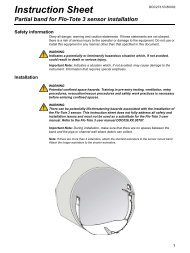
• Partial bands—metal band that covers the bottom half of a channel and stays in<br />
place by attachment to the channel wall. Instruction sheet: DOC273.53.80002.<br />
• Rectangular channel mount—pole with metal plates that stays in place by<br />
attachment to the channel ceiling. Instruction sheet: DOC273.53.80004.<br />
3.3.2 Connection to the <strong>Flo</strong>-Logger, FL900 Series Logger or <strong>Flo</strong>-Station<br />
Connect the cable from the sensor to the <strong>Flo</strong>-Logger, FL900 Series Logger or <strong>Flo</strong>-Station.<br />
• <strong>Flo</strong>-Logger and FL900 Series Logger—connect the cable from the sensor to the<br />
<strong>Flo</strong>-Dar connector on the logger.<br />
• <strong>Flo</strong>-Station—connect the cable from the sensor to the correct terminal in the<br />
<strong>Flo</strong>-Station.<br />
12
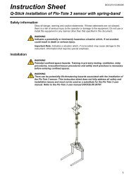
3.4 Dams for low-flow applications<br />
3.4.1 Dam construction<br />
Installation<br />
At least two inches of water is necessary for accurate velocity measurements. If the site<br />
frequently experiences low-flow conditions, use a dam to raise the water level. Locate the<br />
sensor at least one foot in front of the dam.<br />
A low-flow dam can be made as follows:<br />
1. Make a mold for the dam from a section of pipe with the same diameter as the dam<br />
site. Place a board at one end of the pipe, and angle the pipe to approximately 30º<br />
(refer to Figure 5).<br />
2. Pour pre-mixed concrete into the mold. The top of the dam should be 2 inches high.<br />
3. Allow the concrete to fully set.<br />
Figure 5 Low-flow dam construction<br />
1 Board 2 Pre-mix concrete 3 Cut-pipe section<br />
13
Installation<br />
3.4.2 Dam installation<br />
Install the dam at the site, approximately one foot downstream from the sensor. The<br />
easiest way to attach the dam to the pipe or channel is with hydrolytic cement or<br />
waterproof caulking. The dam can also be attached with lead anchors and lag bolts.<br />
Installation options are shown in Figure 6.<br />
Figure 6 Installation options for low-flow dams<br />
1 Low-flow dam 5 Lead anchor<br />
2 <strong>Flo</strong>w sensor 6 Pipe outfall<br />
3 Lag bolt 7 Metal strap<br />
4 Bottom of pipe 8 Metal strap<br />
14
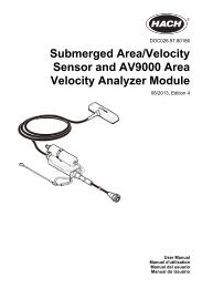
Section 4<br />
Maintenance<br />
4.1 <strong>Sensor</strong> cleaning<br />
WARNING<br />
Potential confined space hazards. Only qualified personnel should conduct the<br />
tasks described in this section of the manual.<br />
Important Note: Do not use sandpaper to clean the non-fouling electrodes. Sandpaper<br />
can damage the electrodes.<br />
1. To clean the sensor, pour a small amount of liquid detergent cleaner on a soft bristle<br />
brush. Use this brush to clean the electrodes on top of the sensor.<br />
2. Rinse with clean water.<br />
Figure 7 Electrodes on <strong>Flo</strong>-<strong>Tote</strong> sensor<br />
1 Ground electrode 2 Velocity electrodes<br />
4.2 Changing the <strong>Sensor</strong> Desiccant<br />
The desiccant canister contains beads of silica gel which ensure proper operation of the<br />
pressure transducer located in the <strong>Tote</strong> 3 sensor. When the beads are yellow, they can<br />
absorb moisture from the air. When they are green, they are saturated and cannot absorb<br />
any more moisture from the air, and they must be replaced immediately.<br />
The cable assembly with desiccant hub is compatible with either the <strong>Flo</strong>-Logger or the<br />
FL900 Loggers. When using this cable assembly with the <strong>Flo</strong>-Logger, do not disconnect<br />
the desiccant cartridge that is attached to the <strong>Flo</strong>-Logger itself.<br />
Important Note: When the beads begin to turn green, replace or rejuvenate the beads.<br />
Permanent damage to the sensor may occur if the desiccant is not maintained. Never<br />
operate the sensor without the proper desiccant. When rejuvenating beads, remove them<br />
from the canister and heat at 100-180 ºC (212-350 ºF) until the beads turn yellow. If the<br />
beads do not turn yellow, replace them with new beads. Do not heat the canister.<br />
4.2.1 Desiccant replacement procedure<br />
Note: Replacing the desiccant does not require that the desiccant container be removed from the<br />
desiccant box.<br />
1. Use a slight twisting motion to twist the bottom end-cap until its slots align with the<br />
retaining clips (Figure 8).<br />
2. Gently remove the end cap by grasping it and pulling it straight out.<br />
3. Pour the desiccant beads out of the canister.<br />
4. Hold the canister up to the light and inspect the hydrophobic filter.<br />
• If you see a small, dim light spot while looking through the hole, the filter is in good<br />
condition. If you see a bright light spot, the filter is probably torn. Replace the filter.<br />
15
Maintenance<br />
• If the desiccant beads were completely saturated with water or the filter has saturated<br />
with water or grease, replace the filter.<br />
5. Refill the canister tube with yellow desiccant beads (Cat. No. 8755500). Inspect the<br />
O-ring (Cat. No. 5252) on the bottom cap for cracking, pits, or evidence of leakage.<br />
Replace if necessary.<br />
Note: Applying O-ring grease to new or dry O-rings improves the ease of insertion, sealing, and life<br />
span of the O-ring.<br />
6. Make sure that the O-ring is clean and free of dirt or debris before replacing the end<br />
cap.<br />
7. Reinstall the end cap.<br />
Figure 8 Remove the bottom end cap<br />
1 End cap 4 Retaining clips<br />
2 Slots for retaining clips 5 Desiccant container<br />
3 O-ring<br />
4.3 Hydrophobic filter description<br />
A single Teflon ® hydrophobic filter (Cat. No. 3390) is installed in the top of the canister to<br />
prevent liquid from entering the vent tube.<br />
16
Maintenance<br />
For best performance and to avoid grease buildup on the filter during submergence or<br />
surcharge conditions, hang the canister vertically so that the end cap points downward<br />
(refer to Figure 8).<br />
Note: The Hydrophobic Filter may need replacement at any time the cartridge is submerged or<br />
exposed to excess moisture. Refer to section 4.4.<br />
4.4 Hydrophobic filter replacement procedure<br />
1. Disconnect the tubing from the top of the desiccant canister.<br />
2. Unscrew the hex-head tubing nipple from the top of the canister and discard the old<br />
filter.<br />
3. Discard any remnants of Teflon tape from the nipple threads. Apply two turns of<br />
Teflon tape (Cat. No. 10854-45) to the threads, pulling the tape into the threads until it<br />
conforms to the shape of the threads.<br />
4. Place a new filter over the hole. Make sure that the smooth side of the filter faces the<br />
inside of the canister.<br />
5. Place the threaded nipple on top of the filter.<br />
6. With slight pressure, press the filter into the hole with the nipple threads and begin<br />
threading the nipple into the hole. The filter will deflect upward and feed completely<br />
into the thread until it disappears. The filter must rotate with the nipple as it is<br />
threaded into the cap. If it does not, it is torn. Start over with a new filter.<br />
7. Inspect the installation. In the upper cap, a small, dim light spot should be visible<br />
when held up to the light. A bright spot indicates a torn filter. Start over with a new<br />
filter.<br />
Figure 9 Replacing the hydrophobic filter<br />
1 Filter, smooth side down 3 Finished assembly<br />
2 Hex-head tubing nipple<br />
17
Maintenance<br />
18
Section 5<br />
Troubleshooting<br />
When a problem occurs, isolate the problem to the sensor, the logger or the interconnect<br />
cable. Some typical problems and solutions are shown in Table 2.<br />
Table 2 Troubleshooting table<br />
Problem Cause Solution<br />
Sudden drops in velocity<br />
Conductivity lost error message<br />
Noisy velocity<br />
Depth measurements are incorrect<br />
or drift<br />
Depth measurements are incorrect<br />
(stuck at zero or at full scale)<br />
The velocity electrodes are covered<br />
with debris.<br />
The velocity electrodes are dry.<br />
The velocity electrodes are covered<br />
with debris or grease.<br />
There may be electrical noise in the<br />
pipe.<br />
Water is in the APR tube.<br />
The internal depth transducer may be<br />
damaged.<br />
Clean the sensor. Make sure the sensor<br />
is installed correctly.<br />
Make sure the water level is above the<br />
sensor. If the water level is low,<br />
construct a low-flow dam.<br />
Clean the sensor.<br />
Identify and eliminate the source of the<br />
interference (if possible).<br />
Replace the desiccant (or APR filter)<br />
cartridge. If possible, remove the sensor<br />
and allow it to dry.<br />
Contact customer support.<br />
19
Troubleshooting<br />
20
Section 6<br />
Contact Information<br />
Ordering information for the U.S.A.<br />
By Telephone:<br />
(800) 368-2723<br />
By Fax:<br />
301-874-8459<br />
By Mail:<br />
Hach Company<br />
4539 Metropolitan Court<br />
Frederick, MD 21704-9452, U.S.A<br />
Ordering information by e-mail:<br />
hachflowsales@hach.com<br />
Information Required<br />
• Hach account number (if available) • Billing address<br />
• Your name and phone number • Shipping address<br />
• Purchase order number • Catalog number<br />
• Brief description or model number • Quantity<br />
European Union<br />
<strong>Flo</strong>w-Tronic<br />
Rue J.H. Cool 19a<br />
B-4840 Welkenraedt<br />
Belgium<br />
Tel: + -32-87-899799<br />
Email: site@flow-tronic.com<br />
www.flow-tronic.com<br />
Outside the U.S.A. and EU<br />
Hach Company maintains a worldwide network of dealers and distributors. To locate the<br />
representative nearest you, send E-mail to hachflowsales@hach.com or visit<br />
www.hachflow.co.<br />
Technical Support<br />
Technical and Customer Service Department personnel are eager to answer questions<br />
about our products and their use. In the U.S.A., call 1-800-368-2723. Outside the U.S.A.<br />
and Europe, send E-mail to hachflowservice@hach.com or call 1-301-874-5599.<br />
Repair Service<br />
Authorization must be obtained from Hach Company before sending any items for repair.<br />
To send the monitor to the factory for repair:<br />
1. Identify the serial number of the sensor.<br />
2. Record the reason for return.<br />
3. Call the Customer Service Department (1-800-368-2723) and get a Service Request<br />
Number (SRN) and shipping label.<br />
4. Use the shipping label provided and ship the equipment in the original packaging if<br />
possible.<br />
Note: Do not ship manuals, computer cables, or other parts with the unit unless they are required for<br />
repair.<br />
21
Contact Information<br />
5. Make sure the equipment is free from foreign debris and is clean and dry before<br />
shipping. <strong>Sensor</strong>s returned without cleaning will be charged a fee.<br />
6. Write the SRN number on the shipping box.<br />
7. Make sure that all return shipments are insured.<br />
8. Address all shipments to:<br />
Hach Company<br />
5600 Lindbergh Drive - North Dock<br />
Loveland, Colorado, 80539-0389 U.S.A.<br />
Attn: SRN#XXX<br />
22
Appendix A Velocity profiling<br />
A.1 About velocity profiling<br />
WARNING<br />
Potential confined space hazards. Only qualified personnel should conduct the<br />
tasks described in this section of the manual.<br />
The sensor measures the water velocity at the bottom of the channel or pipe (called the<br />
sensed velocity). To calculate flow, the user needs to know the average velocity across<br />
the entire channel or pipe cross-section.<br />
The average velocity is different from the sensed velocity because the water moves at<br />
different velocities at different parts of the cross section. The process of correcting the<br />
sensed velocity by measuring the average velocity is called profiling.<br />
Profiling a site involves directly measuring the water velocity at several points across the<br />
pipe cross-section to determine the average velocity. The controller uses this profile<br />
information along with the sensed velocity and depth reported by the flow sensor to<br />
calculate the correct site calibration coefficient for the application.<br />
The sensed velocity and depth should be obtained during or close to the time the velocity<br />
profile was done. The correct site calibration coefficient will allow the average velocity to<br />
be calculated accurately from sensed velocity at all depths.<br />
Note: Because the exact procedure for performing a velocity profile will vary depending on the type<br />
of velocity profiling meter, the information included here is for general purposes. Refer to the user<br />
manual for the velocity profiling meter that is used for specific information.<br />
Figure 10 Typical velocity profile<br />
1 Depth 2 Velocity<br />
23
Velocity profiling<br />
A.2 Site selection<br />
A.3 Profile guidelines<br />
A site which has a typical profile shape will give the most accurate results. For most<br />
cases, sites which may be difficult to profile can be identified by a visual inspection. Use<br />
the following guidelines to select a site:<br />
1. The channel should have as much straight run as possible. Where the length of<br />
straight run is limited, the length upstream from the profile should be twice the<br />
downstream length.<br />
2. The channel should be free of flow disturbances. Look for protruding pipe joints,<br />
sudden changes in diameter, contributing side streams, outgoing side streams, or<br />
obstructions. Clean any rocks, sediment, or other debris that might be on the bottom<br />
of the pipe.<br />
3. The flow should be free of swirls, eddies, vortices, backward flow, or dead zones.<br />
Avoid areas that have visible swirls on the surface.<br />
4. Avoid areas immediately downstream from sharp bends or obstructions.<br />
5. Avoid converging or diverging flow (approach to a flume) and vertical drops.<br />
6. Avoid areas immediately downstream from a sluice gate or where the channel<br />
empties into a body of stationary water.<br />
For best possible results:<br />
1. Measure the horizontal and vertical diameter of the pipe. If there is a difference, then<br />
use the average for the inside diameter of the pipe.<br />
2. Make sure the flow is symmetrical.<br />
3. Measure the depth several times during the procedure.<br />
4. Examine the pipe for rocks, sediment and other debris.<br />
A.4 Depth of flow measurements<br />
To perform a velocity profile, measure the depth of flow in the pipe:<br />
1. Measure the inside diameter of the pipe.<br />
2. Measure the distance from the top of the pipe to the top of the water (Figure 11).<br />
3. Subtract this distance from the inside diameter of the pipe. This is the depth of flow.<br />
Note: The depth and velocities must be measured in the same vertical plane (Figure 12).<br />
24
Velocity profiling<br />
Figure 11 Depth of flow measurement<br />
Figure 12 Depth of flow and velocity profile—single plane<br />
A.5 Velocity profile calculations<br />
A.5.1 .9 x Vmax method<br />
There are four methods for profiling a site. The method chosen depends on the<br />
conditions at the site.<br />
The .9 x Vmax method is the simplest method. Measure the velocity at different points of<br />
the cross section to determine the maximum velocity in the pipe. The average velocity is<br />
calculated by multiplying the maximum velocity by 0.9. This method should be used for:<br />
• Low flows—flows of less than two inches depth.<br />
• Rapidly changing flows—a flow that is changing more than 10% in three<br />
minutes or less can be classified as rapidly changing.<br />
To profile the flow:<br />
1. Measure the velocity at a series of points throughout the entire flow.<br />
2. Identify the fastest velocity. In most cases, this is located in the center just beneath<br />
the surface.<br />
3. Multiply the fastest velocity by 0.9.<br />
25
Velocity profiling<br />
A.5.2 .2, .4, .8 method<br />
The .2, .4, .8 method is the most common method for profiling a typical flow. The velocity<br />
is measured at three points: .2, .4, and .8 times the total depth of flow. The velocity from<br />
each point is entered into the meter. This method should be used for:<br />
• Typical flows—any site which does not have any disturbances, obstructions,<br />
turbulence, etc. Refer to Site selection on page 24.<br />
To profile the flow:<br />
1. Measure the depth of flow (refer to section A.4 on page 24).<br />
2. Calculate the measurement positions on the center line:<br />
• .2 position = 0.2 x depth of flow<br />
• .4 position = 0.4 x depth of flow<br />
• .8 position = 0.8 x depth of flow<br />
3. Measure the velocities at the .2, .4, and .8 positions (Figure 13).<br />
4. Calculate the average of the .2 and .8 velocities.<br />
5. Calculate the average of the .4 velocity with the .2 and .8 average from step 4.<br />
Figure 13 Measurement positions for .2, .4, and .8 method<br />
A.5.3 .4 method<br />
A.5.4 2D method<br />
The .4 method is a simplified version of the .2, .4, .8 method. The velocity is measured at<br />
the .4 position only. Use this method for:<br />
• Low flows—sites free of obstructions, etc., but without sufficient depth to<br />
measure the velocity at three points.<br />
The 2D method uses the velocities from the center line, the vertical velocity lines, and<br />
corners of the flow. Use this method for:<br />
• Asymmetrical flows—sites that have velocities that differ by more than 30% on<br />
either side of the pipe (for example, near a bend).<br />
• Vertical drops—sites that are near an outfall or other change in depth.<br />
• Irregular flows—any site thought to have an irregular or non-typical profile.<br />
26
Velocity profiling<br />
To profile the flow:<br />
1. Find the center line of the flow.<br />
2. Find vertical velocity lines (V V L) that are halfway between the center line and the<br />
side walls of the pipe (refer to Figure 14). Use the widest part of the flow.<br />
3. Measure the velocity at a minimum of 7 different depths along the center line.<br />
4. Measure the velocity along the V V L at different depths. The distance between these<br />
depths should be the same as those on the center line.<br />
5. Measure the velocity at the right and left corners of the flow.<br />
6. Examine the data for any outliers. An outlier will fall outside of the best fit curve<br />
region if a graph were made of the velocity profile.<br />
7. Calculate the average velocity (except outliers) of all measurements (except outliers).<br />
Remember to include the corner measurements.<br />
Figure 14 Velocity profiling for the 2D method<br />
Alternate 2D method<br />
A portable velocity sensor can be used to make a 2D profile. Move the sensor in a swirl<br />
pattern across the entire cross-section (refer to Figure 15). Set the instrument to calculate<br />
the average of these velocity measurements. Refer to the user manual for the portable<br />
velocity sensor for detailed instructions.<br />
Typical procedure (for the <strong>Flo</strong>-Mate velocity profiling meter):<br />
1. Set the FPA time to the appropriate number of seconds.<br />
2. Place the sensor at the start position and wait for a few seconds.<br />
3. Press and start moving the sensor.<br />
27
Velocity profiling<br />
Figure 15 Velocity measured in a swirl pattern<br />
1 Start position 2 Stop position<br />
A.6 Auto-Cal automatic calibration<br />
For sites with straight-run, circular concrete pipes, an Auto-Cal automatic site calibration<br />
can be used in place of velocity profiling.<br />
A.7 Calibrate the sensor using the Cal Wizard in the <strong>Flo</strong>-Ware software<br />
Prerequisite:<br />
The sensor must be installed in the process and must be online in order to perform the<br />
calibration. The sensor can be configured and calibrated with the calibration wizard as<br />
follows:<br />
1. In the <strong>Flo</strong>-Ware software, click on the Programming tab in the FL900 Series Driver<br />
window.<br />
2. Click the <strong>Sensor</strong> Port [1] (sensor name).<br />
3. Click the CAL WIZARD button. The Calibration Wizard window opens.<br />
4. Selec the options on each screen. When the Calibration Complete screen appears,<br />
click FINISH.<br />
5. Click WRITE TO LOGGER to save the settings.<br />
28
Appendix B <strong>Flo</strong>w calculations<br />
B.1 Circular channels<br />
WARNING<br />
Potential confined space hazards. Only qualified personnel should conduct the<br />
tasks described in this section of the manual.<br />
For most applications, the flow in a channel is calculated and recorded by a flow meter.<br />
This appendix is included to calculate the flow manually, or to understand how flow is<br />
calculated.<br />
<strong>Flo</strong>w calculations are provided for:<br />
• Circular channels (section B.1)<br />
• Rectangular channels (section B.2 on page 32)<br />
• Rivers and streams (section B.3 on page 33)<br />
The following values are necessary before the flow can be calculated:<br />
• The average velocity in ft/sec (Appendix A on page 23)<br />
• The depth of flow in inches (in.) at the time of the velocity profile (section A.4 on<br />
page 24)<br />
• The inside diameter of the channel in inches (in.)<br />
1. Calculate the depth to diameter ratio (L/D) where:<br />
• L is the depth of flow in inches at the time of the profile.<br />
• D is the inside diameter in inches.<br />
2. Find the flow unit multiplier (K) from Table 3 on page 30:<br />
a. In the left column, find the L/D ratio from step 1.<br />
b. Move to the right (to the desired units column) to get the flow unit multiplier (K).<br />
Note: Table 3 is for circular conduits only, measured in feet. The multiplier was derived using a<br />
one foot per second flow in a one foot diameter conduit as the model.<br />
3. Convert the diameter to square feet:<br />
• D 2 = (channel diameter in inches ÷ 12) x (channel diameter in inches ÷ 12).<br />
4. Calculate the flow:<br />
• <strong>Flo</strong>w = K x D 2 x average velocity.<br />
Example: What is the flow in millions of gallons per day (MGD) in a 10-inch diameter<br />
channel with a 6-inch depth? The average velocity was found to be 1.5 ft/sec.<br />
L/D = 6 inches/10 inches = 0.6<br />
K = 0.3180<br />
D 2 = (10 in ÷ 12) 2 = (0.833 ft) 2 = 0.694 ft 2<br />
<strong>Flo</strong>w = K x D 2 x average velocity = 0.3180 x 0.694 ft 2 x 1.5 ft/sec = 0.331 MGD<br />
29
<strong>Flo</strong>w calculations<br />
Table 3 <strong>Flo</strong>w unit multiplier<br />
L/D MGD GPM CFS CMM CMD LPM<br />
.01 .0009 .5966 .0013 .0023 3.2522 2.2585<br />
.02 .0024 1.6824 .0037 .0063 9.1709 6.3687<br />
.03 .0044 3.0814 .0069 .0117 16.7986 11.6644<br />
.04 .0068 4.7296 .0105 .0179 25.7811 17.9036<br />
.05 .0095 6.5894 .0147 .0249 35.9190 24.9438<br />
.06 .0124 8.6351 .0192 .0327 47.0701 32.6876<br />
.07 .0156 10.8475 .0242 .0411 59.1295 41.0621<br />
.08 .0190 13.2113 .0294 .0500 72.0148 50.0103<br />
.09 .0226 15.7143 .0350 .0595 85.6585 59.4851<br />
.10 .0264 18.3460 .0409 .0694 100.0039 69.4471<br />
.11 .0304 21.0975 .0470 .0799 115.0022 79.8627<br />
.12 .0345 23.9609 .0534 .0907 130.6108 90.7020<br />
.13 .0388 26.9294 .0600 .1019 146.7919 101.9388<br />
.14 .0432 29.9967 .0668 .1135 163.5116 113.5497<br />
.15 .0477 33.1571 .0739 .1255 180.7393 125.5134<br />
.16 .0524 36.4056 .0811 .1378 198.4467 137.8102<br />
.17 .0572 39.7374 .0885 .1504 216.6081 150.4223<br />
.18 .0621 43.1480 .0961 .1633 235.1995 163.3330<br />
.19 .0672 46.6334 .1039 .1765 254.1985 176.5267<br />
.20 .0723 50.1898 .1118 .1900 273.5844 189.9892<br />
.21 .0775 53.8135 .1199 .2037 293.3373 203.7064<br />
.22 .0828 57.5012 .1281 .2177 313.4387 217.6657<br />
.23 .0882 61.2496 .1365 .2319 333.8710 231.8548<br />
.24 .0937 65.0555 .1449 .2463 354.6172 246.2619<br />
.25 .0992 68.9161 .1535 .2609 375.6613 260.8759<br />
.26 .1049 72.8286 .1623 .2757 396.9880 275.6861<br />
.27 .1106 76.7901 .1711 .2907 418.5825 290.9823<br />
.28 .1163 80.7982 .1800 .3059 440.4305 305.8545<br />
.29 .1222 84.8503 .1890 .3212 462.5182 321.1932<br />
.30 .1281 88.9439 .1982 .3367 484.8325 336.3892<br />
.31 .1340 93.0767 .2074 .3523 507.3605 352.3337<br />
.32 .1400 97.2464 .2167 .3681 530.0894 368.1176<br />
.33 .1461 101.4507 .2260 .3840 553.0071 384.0327<br />
.34 .1522 105.6875 .2355 .4001 576.1017 400.0706<br />
.35 .1583 109.9546 .2450 .4162 599.3618 416.2234<br />
.36 .1645 114.2500 .2545 .4325 622.7757 432.4831<br />
.37 .1707 118.5715 .2642 .4488 646.3325 448.8419<br />
.38 .1770 122.9172 .2739 .4653 670.0208 465.2922<br />
.39 .1833 127.2851 .2836 .4818 693.8301 481.8265<br />
.40 .1896 131.6733 .2934 .4984 717.7501 498.4375<br />
.41 .1960 136.0797 .3032 .5151 741.7607 515.1178<br />
.42 .2023 140.5026 .3130 .5319 765.8788 531.8603<br />
.43 .2087 144.9400 .3229 .5487 790.0673 548.6578<br />
30
<strong>Flo</strong>w calculations<br />
Table 3 <strong>Flo</strong>w unit multiplier (continued)<br />
L/D MGD GPM CFS CMM CMD LPM<br />
.44 .2151 149.3902 .3328 .5655 814.3250 565.5034<br />
.45 .2215 153.8512 .3428 .5824 838.6420 582.3902<br />
.46 .2280 158.3212 .3527 .5993 863.0080 599.3111<br />
.47 .2344 162.7985 .3627 .6163 887.4133 616.2592<br />
.48 .2409 167.2811 .3727 .6332 911.8480 633.2277<br />
.49 .2473 171.7673 .3827 .6502 936.3024 650.2100<br />
.50 .2538 176.2553 .3927 .6672 960.7664 667.1989<br />
.51 .2603 180.7433 .4027 .6842 985.2306 684.1879<br />
.52 .2667 185.2295 .4127 .7012 1009.6850 701.1701<br />
.53 .2732 189.7121 .4227 .7181 1043.1200 718.1385<br />
.54 .2796 194.1894 .4327 .7351 1058.5250 735.0869<br />
.55 .2861 198.6594 .4426 .7520 1082.8910 752.0076<br />
.56 .2925 203.1204 .4526 .7689 1107.1080 768.8945<br />
.57 .2989 207.5706 .4635 .7857 1131.4660 785.7401<br />
.58 .3053 212.0080 .4724 .8025 1155.6540 802.5377<br />
.59 .3117 216.4309 .4822 .8193 1179.7630 819.2801<br />
.60 .3180 220.8374 .4920 .8360 1203.7830 835.9605<br />
.61 .3243 225.2255 .5018 .8526 1227.7030 852.5715<br />
.62 .3306 229.5934 .5115 .8691 1251.5120 869.1057<br />
.63 .3369 233.9392 .5212 .8856 1275.2010 885.5560<br />
.64 .3431 238.2607 .5308 .9019 1298.7580 901.9149<br />
.65 .3493 242.5560 .5404 .9182 1322.1710 918.1745<br />
.66 .3554 246.8232 .5499 .9343 1345.4320 934.3275<br />
.67 .3615 251.0600 .5594 .9504 1368.5260 950.3654<br />
.68 .3676 255.2643 .5687 .9663 1391.4440 966.2805<br />
.69 .3736 259.4340 .5780 .9821 1414.1730 982.0645<br />
.70 .3795 263.5668 .5872 .9977 1436.7010 997.7090<br />
.71 .3854 267.6604 .5963 1.0132 1459.0150 1013.2050<br />
.72 .3913 271.7125 .6054 1.0285 1481.1030 1028.5440<br />
.73 .3970 275.7206 .6143 1.0437 1502.9510 1043.7160<br />
.74 .4027 279.6822 .6231 1.0579 1524.5460 1058.7120<br />
.75 .4084 283.5946 .6319 1.0735 1545.8720 1073.5220<br />
.76 .4139 287.4553 .6405 1.0881 1566.9170 1088.1370<br />
.77 .4194 291.2612 .6489 1.1025 1587.6630 1102.5440<br />
.78 .4248 295.0096 .6573 1.1167 1608.0950 1116.7330<br />
.79 .4301 298.6972 .6655 1.1307 1628.1970 1130.6920<br />
.80 .4353 302.3210 .6736 1.1444 1647.9500 1144.4090<br />
.81 .4405 305.8774 .6815 1.1579 1667.3360 1157.8720<br />
.82 .4455 309.3629 .6893 1.1711 1686.3350 1171.0660<br />
.83 .4505 312.7735 .6969 1.1840 1704.9260 1183.9760<br />
.84 .4552 316.1053 .7043 1.1966 1723.0880 1196.5890<br />
.85 .4599 319.3538 .7115 1.2089 1740.7950 1208.8860<br />
.86 .4644 322.5143 .7186 1.2208 1758.0230 1220.8490<br />
.87 .4688 325.5815 .7254 1.2325 1774.7430 1232.4600<br />
31
<strong>Flo</strong>w calculations<br />
Table 3 <strong>Flo</strong>w unit multiplier (continued)<br />
L/D MGD GPM CFS CMM CMD LPM<br />
.88 .4731 328.5500 .7320 1.2437 1790.9240 1243.6970<br />
.89 .4772 331.4135 .7384 1.2545 1806.5330 1254.5360<br />
.90 .4812 334.1650 .7445 1.2650 1821.5310 1264.9520<br />
.91 .4850 336.7967 .7504 1.2749 1835.8760 1274.9140<br />
.92 .4886 339.2997 .7560 1.2844 1849.5200 1284.3890<br />
.93 .4920 341.6636 .7612 1.2933 1862.4060 1293.3370<br />
.94 .4952 343.8759 .7662 1.3017 1874.4650 1301.7120<br />
.95 .4981 345.9216 .7707 1.3095 1885.6160 1309.4560<br />
.96 .5008 347.7815 .7749 1.3165 1895.7540 1316.4960<br />
.97 .5032 349.4297 .7785 1.3277 1904.7390 1322.7350<br />
.98 .5052 350.8287 .7816 1.3280 1912.3650 1328.0310<br />
.99 .5068 351.9145 .7841 1.3321 1918.2840 1332.1410<br />
1.00 .5076 352.5112 .7854 1.3344 1921.5360 1334.4000<br />
B.2 Rectangular channels<br />
<strong>Flo</strong>w in rectangular channels is calculated as follows:<br />
1. Find the average velocity with the 0.2, 0.4, 0.8 method (refer to section A.5.2 on<br />
page 26).<br />
Note: For channel widths that are six feet or more, use the .2, .6, .8 method as described for<br />
rivers and streams (section B.3 on page 33). Velocity units must be in ft/sec.<br />
2. Calculate the cross-sectional area in square feet (ft 2 ):<br />
• Area = [(depth of flow) in. ÷ 12] x [(channel width) in. ÷ 12]<br />
3. Calculate the flow:<br />
• Average velocity x cross-sectional area<br />
The result will be a flow rate in ft 3 /sec (CFS). For conversion to other flow units, refer<br />
to section B.4 on page 35.<br />
Example: What is the flow in millions of gallons per day (MGD) in a rectangular channel<br />
that is 24 inches wide and has a 10-inch deep flow?<br />
Average velocity:<br />
Velocity at .2 x depth (2 inches) = 1.5 ft/sec<br />
Velocity at .4 x depth (4 inches) = 1.7 ft/sec<br />
Velocity at .8 x depth (8 inches) = 1.8 ft/sec<br />
(1.5 + 1.8) ÷ 2 = 1.65 ft/sec<br />
Average velocity = (1.65 + 1.7) ÷ 2 = 1.67 ft/sec<br />
Cross-sectional area:<br />
Convert inches to feet: 10 in ÷ 12 = 0.83 ft<br />
Area = 0.83 ft x 2 ft = 1.66 ft 2<br />
<strong>Flo</strong>w = 1.67 ft 2 /sec x 1.66 ft = 2.77 ft 3 /sec<br />
From Table 4 on page 35, 2.77 ft 3 /sec x 0.64632 = 1.7903 MGD<br />
32
B.3 Rivers and streams<br />
<strong>Flo</strong>w calculations<br />
1. Find the depth of each segment of the channel:<br />
a. Divide the width of the channel into segments of equal length (d). Refer to<br />
Figure 16 on page 34.<br />
b. Locate the center line of each segment (½ x d).<br />
c. Measure the depth of each segment on the segment center line.<br />
Note: The .2, .6, and .8 positions for rivers and streams are measured from the surface. All<br />
depth and velocity measurements must be on the same plane.<br />
Note: Smaller segments will give better results. If the difference in mean velocity between two<br />
adjacent segments is greater than 10%, make the segments smaller.<br />
2. Use a velocity profile to calculate the flow for each segment:<br />
a. Calculate the .2, .6, .8 velocity positions on the center line of each segment.<br />
b. Measure the velocity at the .2, .6, and .8 positions.<br />
c. Calculate the average of the .2 and .8 velocities.<br />
d. Calculate the average of the .6 velocity and the average of the .2 and .8 velocities.<br />
This is the average velocity.<br />
e. Calculate the cross-sectional area of each segment. Refer to Figure 17 on<br />
page 34.<br />
f. Calculate the flow of each segment:<br />
<strong>Flo</strong>w = segment area x average velocity<br />
3. Add the flows of all of the segments. The total flow for the river or stream is the sum<br />
of the segment flows.<br />
33
<strong>Flo</strong>w calculations<br />
Figure 16 Segments for a river or stream<br />
Figure 17 Segment area calculations<br />
1 Trapezoid 2 Rectangle<br />
34
B.4 <strong>Flo</strong>w unit conversions<br />
<strong>Flo</strong>w calculations<br />
1. Find the original unit in the left column of Table 4.<br />
2. Find the new unit in the top row of Table 4.<br />
3. Find the table cell where the units intersect. This is the conversion factor.<br />
4. Multiply the original value by the conversion factor to get the value in terms of the<br />
new unit.<br />
Example: convert 20 ft 3 /sec (CFS) to million gallons per day (MGD).<br />
From Table 4, the conversion factor from CFS to MGD is 0.64632.<br />
20 ft 3 /sec x 0.64632 = 12.9 MGD<br />
Table 4 <strong>Flo</strong>w unit conversion factors<br />
To (new units)<br />
From<br />
(original units)<br />
CFS MGD GPM CMD CMM<br />
CFS 1 0.64632 448.831 2446.576 1.69901<br />
MGD 1.54723 1 694.44 3785.412 2.62876<br />
GPM 0.002228 0.00144 1 5.45099 0.0037854<br />
CMD 0.000408 0.0002642 0.18345 1 0.0006944<br />
CMM 0.5885 0.380408 264.172 1440 1<br />
<strong>Flo</strong>w units:<br />
Unit<br />
MGD =<br />
GPM =<br />
CFS =<br />
CMM =<br />
CMD =<br />
LPM =<br />
Definition<br />
million gallons per day<br />
gallons per minute<br />
cubic feet per second<br />
cubic meters per minute<br />
cubic meters per day<br />
liters per minute<br />
35
<strong>Flo</strong>w calculations<br />
36
Index<br />
A<br />
accuracy problems ................................................... 19<br />
APR tube ................................................................... 8<br />
area, cross-sectional ................................................ 32<br />
C<br />
cleaning ................................................................... 15<br />
concrete mold for dams ........................................... 13<br />
confined space entry .................................................. 6<br />
conversion factors .................................................... 35<br />
D<br />
dam construction for low flow .................................. 13<br />
depth measurement ................................................... 8<br />
depth of flow measurement ..................................... 24<br />
E<br />
electrodes .................................................................. 7<br />
errors ....................................................................... 19<br />
F<br />
Faraday’s law ............................................................. 7<br />
flow rate calculation ................................................... 8<br />
circular channels ............................................... 29<br />
rectangular channel ........................................... 32<br />
rivers and streams ............................................. 33<br />
flow unit multipliers .................................................. 30<br />
I<br />
installation .................................................................. 9<br />
installation kits ......................................................... 12<br />
K<br />
K, flow unit multiplier ................................................ 30<br />
L<br />
L/D ratio ................................................................... 29<br />
location guidelines ..................................................... 9<br />
low-flow applications ................................................ 13<br />
M<br />
measurement<br />
depth ................................................................... 8<br />
velocity ................................................................ 7<br />
P<br />
parts ........................................................................... 9<br />
S<br />
safety information ....................................................... 5<br />
sensor locations ......................................................... 9<br />
specifications ............................................................. 3<br />
T<br />
theory of operation ..................................................... 7<br />
troubleshooting ........................................................ 19<br />
U<br />
units, flow ................................................................. 35<br />
V<br />
velocity measurement ................................................ 7<br />
velocity profile<br />
0.4 method ........................................................ 26<br />
0.9 Vmax method .............................................. 25<br />
2D method ......................................................... 26<br />
about ................................................................. 23<br />
methods ............................................................. 25<br />
37
Index<br />
38