The care and feeding of digital, pulse-shaping ... - Nonstop Systems
The care and feeding of digital, pulse-shaping ... - Nonstop Systems
The care and feeding of digital, pulse-shaping ... - Nonstop Systems

You also want an ePaper? Increase the reach of your titles
YUMPU automatically turns print PDFs into web optimized ePapers that Google loves.
mixed signal<br />
<strong>The</strong> <strong>care</strong> <strong>and</strong> <strong>feeding</strong><br />
<strong>of</strong> <strong>digital</strong>,<br />
<strong>pulse</strong>-<strong>shaping</strong> filters<br />
In the not-too-distant future,<br />
data will be the predominant<br />
baggage carried by wireless<br />
<strong>and</strong> other transmission systems.<br />
Pulse-<strong>shaping</strong> filters will<br />
play a critical part<br />
in maintaining signal integrity.<br />
By Ken Gentile<br />
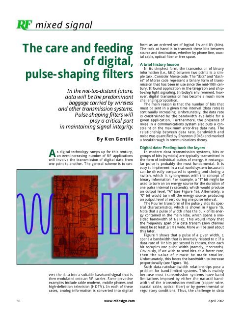
As <strong>digital</strong> technology ramps up for this century,<br />
an ever-increasing number <strong>of</strong> RF applications<br />
will involve the transmission <strong>of</strong> <strong>digital</strong> data from<br />
one point to another. <strong>The</strong> general scheme is to convert<br />
the data into a suitable baseb<strong>and</strong> signal that is<br />
then modulated onto an RF carrier. Some pervasive<br />
examples include cable modems, mobile phones <strong>and</strong><br />
high-definition television (HDTV). In each <strong>of</strong> these<br />
cases, analog information is converted into <strong>digital</strong><br />
form as an ordered set <strong>of</strong> logical 1’s <strong>and</strong> 0’s (bits).<br />
<strong>The</strong> task at h<strong>and</strong> is to transmit these bits between<br />
source <strong>and</strong> destination, whether by phone line, coaxial<br />
cable, optical fiber or free space.<br />
A brief history lesson<br />
In its simplest form, the transmission <strong>of</strong> binary<br />
information (i.e., bits) between two points is a simple<br />
task. Consider Morse code. <strong>The</strong> “dots” <strong>and</strong> “dashes”<br />
<strong>of</strong> Morse code represent a binary form <strong>of</strong> transmission<br />
that has been in use since the mid-19th century.<br />
It found application in the telegraph <strong>and</strong> shipto-ship<br />
light signaling. In today’s environment, however,<br />
<strong>digital</strong> transmission has become a much more<br />
challenging proposition.<br />
<strong>The</strong> main reason is that the number <strong>of</strong> bits that<br />
must be sent in a given time interval (data rate) is<br />
continually increasing. Unfortunately, the data rate<br />
is constrained by the b<strong>and</strong>width available for a<br />
given application. Furthermore, the presence <strong>of</strong><br />
noise in a communications system also puts a constraint<br />
on the maximum error-free data rate. <strong>The</strong><br />
relationship between data rate, b<strong>and</strong>width <strong>and</strong><br />
noise was quantified by Shannon (1948) <strong>and</strong> marked<br />
a breakthrough in communications theory.<br />
Digital data: Peeling back the layers<br />
In modern data transmission systems, bits or<br />
groups <strong>of</strong> bits (symbols) are typically transmitted in<br />
the form <strong>of</strong> individual <strong>pulse</strong>s <strong>of</strong> energy. A rectangular<br />
<strong>pulse</strong> is probably the most fundamental. It is<br />
easy to implement in a real-world system because it<br />
can be directly compared to opening <strong>and</strong> closing a<br />
switch, which is synonymous with the concept <strong>of</strong><br />
binary information. For example, a “1” bit might be<br />
used to turn on an energy source for the duration <strong>of</strong><br />
one <strong>pulse</strong> interval (τ seconds), which would produce<br />
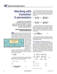
an output level, “A” (see Figure 1a). Alternately, a<br />
“0” bit would turn <strong>of</strong>f the energy source, producing<br />
an output level <strong>of</strong> zero during one <strong>pulse</strong> interval.<br />
<strong>The</strong> Fourier transform <strong>of</strong> the <strong>pulse</strong> yields its spectral<br />
characteristics, which is shown in Figure 1b.<br />
Note that a <strong>pulse</strong> <strong>of</strong> width τ has the bulk <strong>of</strong> its energy<br />
contained in the main lobe, which spans a onesided<br />
b<strong>and</strong>width <strong>of</strong> 1/τ Hz. This would imply that<br />
the frequency span <strong>of</strong> a data transmission channel<br />
must be at least 2/τ Hz wide. More will be said about<br />
this later.<br />
Figure 1 shows that a <strong>pulse</strong> <strong>of</strong> a given width, τ,<br />
spans a b<strong>and</strong>width that is inversely related to τ. If a<br />
data rate <strong>of</strong> 1/τ bits per second is chosen, then each<br />
bit occupies one <strong>pulse</strong> width (namely, τ seconds).<br />
Obviously, if we wish to send bits at a faster rate,<br />
then the value <strong>of</strong> τ must be made smaller.<br />
Unfortunately, this forces the b<strong>and</strong>width to increase<br />
proportionally (see Figure. 1b).<br />
Such data-rate/b<strong>and</strong>width relationships pose a<br />
problem for b<strong>and</strong>-limited systems. This is mainly<br />
because most transmission systems have b<strong>and</strong><br />
limitations imposed by either the natural b<strong>and</strong>width<br />
<strong>of</strong> the transmission medium (copper wire,<br />
coaxial cable, optical fiber) or by governmental or<br />
regulatory conditions. Thus, the challenge in data<br />
50 www.rfdesign.com April 2002
transmission systems is to obtain the<br />
highest possible data rate in the b<strong>and</strong>width<br />
allotted with the least number<br />
<strong>of</strong> errors (preferably none).<br />
Pulse <strong>shaping</strong>: <strong>The</strong> details<br />
Before delving into the details <strong>of</strong><br />
<strong>pulse</strong> <strong>shaping</strong>, it is important to underst<strong>and</strong><br />
that <strong>pulse</strong>s are sent by the transmitter<br />
<strong>and</strong> ultimately detected by the<br />
receiver in any data transmission system.<br />
At the receiver, the goal is to sample<br />
the received signal at an optimal<br />
point in the <strong>pulse</strong> interval to maximize<br />
the probability <strong>of</strong> an accurate binary<br />
Figure 1. A single rectangular <strong>pulse</strong> <strong>and</strong> its<br />
Fourier transform.<br />
decision. This implies that the fundamental<br />
shapes <strong>of</strong> the <strong>pulse</strong>s be such<br />
that they do not interfere with one<br />
another at the optimal sampling point.<br />
<strong>The</strong>re are two criteria that ensure<br />
noninterference. Criterion one is that<br />
the <strong>pulse</strong> shape exhibits a zero crossing<br />
at the sampling point <strong>of</strong> all <strong>pulse</strong> intervals<br />
except its own. Otherwise, the<br />
residual effect <strong>of</strong> other <strong>pulse</strong>s will introduce<br />
errors into the decision making<br />
process. Criterion two is that the shape<br />
<strong>of</strong> the <strong>pulse</strong>s be such that the amplitude<br />
decays rapidly outside <strong>of</strong> the <strong>pulse</strong><br />
interval.<br />
This is important because any real<br />
system will contain timing jitter,<br />
which means that the actual sampling<br />
point <strong>of</strong> the receiver will not always be<br />
optimal for each <strong>and</strong> every <strong>pulse</strong>. So,<br />
even if the <strong>pulse</strong> shape provides a zero<br />
crossing at the optimal sampling point<br />
<strong>of</strong> other <strong>pulse</strong> intervals, timing jitter<br />
in the receiver could cause the sampling<br />
instant to move, thereby missing<br />
the zero crossing point. This, too,<br />
introduces error into the decisionmaking<br />
process. Thus, the quicker a<br />
<strong>pulse</strong> decays outside <strong>of</strong> its <strong>pulse</strong> interval,<br />
the less likely it is to allow timing<br />
jitter to introduce errors when sampling<br />
adjacent <strong>pulse</strong>s. In addition to<br />
the noninterference criteria, there is<br />
the ever-present need to limit the<br />
<strong>pulse</strong> b<strong>and</strong>width, as explained earlier.<br />
<strong>The</strong> rectangular <strong>pulse</strong><br />
<strong>The</strong> rectangular <strong>pulse</strong>, by definition,<br />
meets criterion number one because it<br />
is zero at all points outside <strong>of</strong> the present<br />
<strong>pulse</strong> interval. It clearly cannot<br />
cause interference during the sampling<br />
time <strong>of</strong> other <strong>pulse</strong>s. <strong>The</strong> trouble with<br />
the rectangular <strong>pulse</strong>, however, is that<br />
it has significant energy over a fairly<br />
large b<strong>and</strong>width as indicated by its<br />
Fourier transform (see Figure 1b). In<br />
fact, because the spectrum <strong>of</strong> the <strong>pulse</strong><br />
is given by the familiar sin(πx)/πx (sinc)<br />
response, its b<strong>and</strong>width actually<br />
extends to infinity. <strong>The</strong> unbounded frequency<br />
response <strong>of</strong> the rectangular<br />
<strong>pulse</strong> renders it unsuitable for modern<br />
transmission systems. This is where<br />
<strong>pulse</strong> <strong>shaping</strong> filters come into play.<br />
If the rectangular <strong>pulse</strong> is not the<br />
best choice for b<strong>and</strong>-limited data transmission,<br />
then what <strong>pulse</strong> shape will<br />
limit b<strong>and</strong>width, decay quickly, <strong>and</strong><br />
provide zero crossings at the <strong>pulse</strong> sampling<br />
times? <strong>The</strong> raised cosine <strong>pulse</strong>,<br />
which is used in a wide variety <strong>of</strong> modern<br />
data transmission systems. <strong>The</strong><br />
magnitude spectrum, P(ω), <strong>of</strong> the raised<br />
cosine <strong>pulse</strong> is given by:<br />
( 1) P( ω)=<br />
τ<br />
( 1 − )<br />
for 0 ≤ω ≤<br />
π α<br />
τ<br />
τ⎛<br />
( ) ( )=<br />
2 1 ⎛ ⎛ τ ⎞ ⎛ ⎞<br />
2 P ω −sin<br />
⎝<br />
⎜<br />
2 ⎠<br />
⎟ −<br />
⎝<br />
⎜<br />
α ω π ⎞ ⎞<br />
τ ⎠<br />
⎟<br />
⎝<br />
⎜<br />
⎠<br />
⎟<br />
⎝<br />
⎜<br />
⎠<br />
⎟<br />
for<br />
π( 1-α) ( 1+ )<br />
≤ ω π α ≤<br />
τ<br />
τ<br />
( 3 ) P( ω)=<br />
0<br />
for ≥ ( 1+<br />
ω π α )<br />
τ<br />
(1)<br />
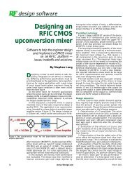
<strong>The</strong> spectral shape <strong>of</strong> the raised cosine<br />
<strong>pulse</strong> is shown in Figure 2a. <strong>The</strong><br />
inverse Fourier transform <strong>of</strong> P(ω) yields<br />
the time-domain response, p(t), <strong>of</strong> the<br />
raised cosine <strong>pulse</strong> (see Figure 2b). This<br />
is also referred to as the im<strong>pulse</strong><br />
response <strong>and</strong> is given by:<br />
⎛ t⎞<br />
t<br />
⎝<br />
⎜<br />
⎠<br />
⎟ ⎛ ⎝ ⎜<br />
απ ⎞<br />
sinc cos<br />
⎠<br />
⎟<br />
τ τ<br />
pt ( )=<br />
t<br />
− ⎛ 2<br />
⎝ ⎜<br />
2α<br />
⎞<br />
1<br />
⎠<br />
⎟<br />
τ<br />
(2)<br />
Care must be taken when (2) is used<br />
for calculation because the denominator<br />
can go to zero if αt/τ = ±½. <strong>The</strong>refore,<br />
any program used to compute p(t) must<br />
test for the occurrence <strong>of</strong> αt/τ = ±½.<br />
Because it can be shown that the limit<br />
<strong>of</strong> p(t) as αt/τ approaches ±½ is given by<br />
(π/4) sinc(t/τ), this is the formula to use<br />
when the special case <strong>of</strong> αt/τ = ±½ is<br />
encountered.<br />
<strong>The</strong> raised cosine <strong>pulse</strong><br />
Unlike the rectangular <strong>pulse</strong>, the<br />
raised cosine <strong>pulse</strong> takes on the shape<br />
<strong>of</strong> a sinc <strong>pulse</strong>, as indicated by the leftmost<br />
term <strong>of</strong> p(t). Unfortunately, the<br />
name “raised cosine” is misleading. It<br />
actually refers to the <strong>pulse</strong>’s frequency<br />
spectrum, P(ω), not to its time domain<br />
shape, p(t). <strong>The</strong> precise shape <strong>of</strong> the<br />
raised cosine spectrum is determined by<br />
the parameter, α, where 0 ≤ α ≤ 1.<br />
Specifically, α governs the b<strong>and</strong>width<br />
occupied by the <strong>pulse</strong> <strong>and</strong> the rate at<br />
which the tails <strong>of</strong> the <strong>pulse</strong> decay. A<br />
value <strong>of</strong> α = 0 <strong>of</strong>fers the narrowest<br />
b<strong>and</strong>width, but the slowest rate <strong>of</strong><br />
decay in the time domain. When α = 1,<br />
Figure 2. Spectral shape <strong>and</strong> inverse Fourier<br />
transform <strong>of</strong> the raised cosine <strong>pulse</strong>.<br />
52 www.rfdesign.com April 2002
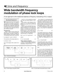
Figure 3. Interaction <strong>of</strong> raised cosine <strong>pulse</strong>s<br />
when the time between <strong>pulse</strong>s coincides with<br />
the data rate.<br />
Figure 4. <strong>The</strong> functional form <strong>of</strong> FIR <strong>and</strong> IIR<br />
filters.<br />
the b<strong>and</strong>width is 1/τ, but the time<br />
domain tails decay rapidly. It is interesting<br />
to note that the α = 1 case <strong>of</strong>fers<br />
a double-sided b<strong>and</strong>width <strong>of</strong> 2/τ. This<br />
exactly matches the b<strong>and</strong>width <strong>of</strong> the<br />
main lobe <strong>of</strong> a rectangular <strong>pulse</strong>, but<br />
with the added benefit <strong>of</strong> rapidly decaying<br />
time-domain tails. Conversely,<br />
inverse when α = 0, the b<strong>and</strong>width is<br />
reduced to 1/τ, implying a factor-<strong>of</strong>-two<br />
increase in data rate for the same b<strong>and</strong>width<br />
occupied by a rectangular <strong>pulse</strong>.<br />
However, this comes at the cost <strong>of</strong> a<br />
much slower rate <strong>of</strong> decay in the tails <strong>of</strong><br />
the <strong>pulse</strong>. Thus, the parameter α gives<br />
the system designer a trade-<strong>of</strong>f between<br />
increased data rate <strong>and</strong> time-domain<br />
tail suppression. <strong>The</strong> latter is <strong>of</strong> prime<br />
importance for systems with relatively<br />
high timing jitter at the receiver.<br />
Figure 3 shows how a train <strong>of</strong> raised<br />
cosine <strong>pulse</strong>s interact when the time<br />
between <strong>pulse</strong>s coincides with the data<br />
rate. Note how the zero crossings are<br />
coincident with the <strong>pulse</strong> centers (the<br />
sampling point) as desired.<br />
It should be pointed out that the<br />
raised cosine <strong>pulse</strong> is not a cure-all. Its<br />
application is restricted to energy <strong>pulse</strong>s<br />
that are real <strong>and</strong> even (i.e., symmetric<br />
about t = 0). A different form <strong>of</strong> <strong>pulse</strong><br />
<strong>shaping</strong> is required for <strong>pulse</strong>s that are<br />
not real <strong>and</strong> even. However, regardless<br />
<strong>of</strong> the necessary <strong>pulse</strong> shape, once it is<br />
expressible in either the time or frequency<br />
domain, the process <strong>of</strong> designing<br />
a <strong>pulse</strong>-<strong>shaping</strong> filter remains the<br />
same. In this article, only the raised<br />
cosine <strong>pulse</strong> shape will be considered.<br />
A variant <strong>of</strong> the raised cosine <strong>pulse</strong> is<br />
<strong>of</strong>ten used in modern systems – the<br />
root-raised cosine response. <strong>The</strong> frequency<br />
response is expressed simply as<br />
the square root <strong>of</strong> P(ω) (<strong>and</strong> square root<br />
<strong>of</strong> p(t) in the time domain). This shape<br />
is used when it is desirable to share the<br />
<strong>pulse</strong>-<strong>shaping</strong> load between the transmitter<br />
<strong>and</strong> receiver.<br />
It’s better in <strong>digital</strong><br />
Before the advent <strong>of</strong> <strong>digital</strong> filter<br />
design, <strong>pulse</strong>-<strong>shaping</strong> filters had to be<br />
implemented as analog filter designs.<br />
Digital filters, however, <strong>of</strong>fer several<br />
advantages <strong>of</strong> analog designs. <strong>The</strong>y can<br />
be integrated directly on silicon, which<br />
makes them attractive for system-on-achip<br />
(SoC) designs. Furthermore, the<br />
problem <strong>of</strong> component drift due to temperature<br />
<strong>and</strong> aging is eliminated. Also,<br />
their spectral characteristics are consistent<br />
<strong>and</strong> reproducible <strong>and</strong> do not suffer<br />
from component tolerance issues.<br />
With the plethora <strong>of</strong> <strong>digital</strong> filter<br />
design tools available on the market,<br />
the designer can design a variety <strong>of</strong> <strong>digital</strong><br />
filters with little effort.<br />
Choices, choices, choices<br />
Given that the <strong>pulse</strong> shape has been<br />
defined mathematically (such as the<br />
raised cosine <strong>pulse</strong>), the next task is to<br />
decide which basic category <strong>of</strong> <strong>digital</strong><br />
filter to use: finite im<strong>pulse</strong> response<br />
(FIR) or infinite im<strong>pulse</strong> response (IIR).<br />
<strong>The</strong> functional form <strong>of</strong> FIR <strong>and</strong> IIR<br />
filters is shown in Figure 4. <strong>The</strong> fundamental<br />
difference between them is the<br />
fact that the IIR contains feedback. This<br />
should be obvious from the fact that the<br />
b i coefficient’s feedback scaled <strong>and</strong><br />
delayed samples <strong>of</strong> the output y(n).<br />
Hence, the history <strong>of</strong> the output affects<br />
the future <strong>of</strong> the output. This is not true<br />
for the FIR, where y(n) only depends on<br />
the history <strong>of</strong> the input samples, x(n).<br />
<strong>The</strong> implication is that the response <strong>of</strong><br />
an IIR filter to an im<strong>pulse</strong> (a single nonzero<br />
sample followed by zero samples) is<br />
infinite. That is, the IIR will continue to<br />
produce non-zero output samples long<br />
after the application <strong>of</strong> an im<strong>pulse</strong>. This<br />
is an undesirable consequence for data<br />
Figure 5. An arbitrary <strong>digital</strong> filter frequency<br />
response.<br />
<strong>pulse</strong> transmission (recall the noninterference<br />
criteria).<br />
<strong>The</strong> FIR does not suffer from this<br />
problem because its architecture does<br />
not contain any feedback elements. A<br />
single, non-zero im<strong>pulse</strong> at the input<br />
will only yield output samples while the<br />
im<strong>pulse</strong> propagates down the delay<br />
stages. Generally, <strong>pulse</strong> <strong>shaping</strong> filters<br />
employ FIR designs.<br />
<strong>The</strong> basic building blocks <strong>of</strong> a <strong>digital</strong><br />
filter are adders (⊕), multipliers (⊗),<br />
<strong>and</strong> unit-delays (D); all <strong>of</strong> which can be<br />
readily implemented in <strong>digital</strong> form.<br />
Adders <strong>and</strong> multipliers are composed <strong>of</strong><br />
combinational logic while the unit<br />
delays are composed <strong>of</strong> latches (which<br />
require a clock signal). <strong>The</strong> basic filtering<br />
operation consists <strong>of</strong> a sequence <strong>of</strong><br />
multiply/add/delay operations that<br />
occur each time the delay stages are<br />
clocked. This is effectively a convolution<br />
operation, which may be expressed as:<br />
y(n) = x(n) * h(n)<br />
In this expression, * is the convolution<br />
operator <strong>and</strong> should not be taken to<br />
mean simple multiplication. <strong>The</strong><br />
Fourier transform (or z-transform in the<br />
case <strong>of</strong> <strong>digital</strong> filters) reveals that filtering<br />
is synonymous with convolution.<br />
This is the “secret” <strong>of</strong> <strong>digital</strong> filters —<br />
by using relatively simple operations<br />
(add/multiply/delay), a filtering operation<br />
can be realized. <strong>The</strong> trick, <strong>of</strong><br />
course, is coming up with the proper<br />
Figure 6. Converting an im<strong>pulse</strong> to a raised<br />
cosine <strong>pulse</strong> by filtering.<br />
54 www.rfdesign.com April 2002
Typically, this is determined by the<br />
number <strong>of</strong> bit (or symbol) intervals<br />
that the designer would like the filter<br />
response to occupy.<br />
Remember, an FIR filter im<strong>pulse</strong><br />
response lasts only as long as the<br />
number <strong>of</strong> taps. If the filter oversamples<br />
by a factor <strong>of</strong> two <strong>and</strong> the desired<br />
im<strong>pulse</strong> response duration is five bits<br />
(or symbols), then 10 taps are required<br />
(2 x 5 = 10). Obviously, a trade-<strong>of</strong>f<br />
exists between the number <strong>of</strong> taps (circuit<br />
complexity) <strong>and</strong> the filter’s<br />
response characteristic.<br />
Figure 7. <strong>The</strong> frequency responses <strong>of</strong> two different versions <strong>of</strong> the raised cosine <strong>pulse</strong>-<strong>shaping</strong> filter.<br />
h(n) to produce the desired filtering<br />
operation (i.e., spectral <strong>shaping</strong> in the<br />
frequency domain). This is another topic<br />
altogether, but the many <strong>digital</strong> filter<br />
design tools that are available today<br />
make this process easier than ever<br />
before. <strong>The</strong>se design tools give the<br />
designer the ability to generate the necessary<br />
filter coefficients for a desired<br />
frequency response (or vice versa).<br />
Other variables that enter into the<br />
design process include determining the<br />
optimal number <strong>of</strong> filter coefficients <strong>and</strong><br />
how much numeric precision (resolution)<br />
is required to get the job done.<br />
Resolution refers to the number <strong>of</strong><br />
bits used to represent the coefficient<br />
values, as well as the number <strong>of</strong> bits<br />
used to represent the sample values at<br />
any given point in the filter. Resolution<br />
affects the overall complexity <strong>of</strong> the<br />
design because more bits means more<br />
<strong>digital</strong> hardware.<br />
How it comes together<br />
Before proceeding with a design<br />
example, it should be noted from Figure<br />
4b that h(n) (the im<strong>pulse</strong> response <strong>of</strong><br />
the filter) is directly determined by the<br />
filter coefficients. This can be used to an<br />
advantage in the filter design process,<br />
because an outcome <strong>of</strong> the FIR filter<br />
design process is the im<strong>pulse</strong> response,<br />
h(n). <strong>The</strong> h(n) values can be directly<br />
substituted for the a i coefficients.<br />
response is shown in Figure 5. Now<br />
recall the raised cosine response (see<br />
Figure 2a), which can extend out to a<br />
frequency <strong>of</strong> 1/τ (for α = 1). If one were<br />
to operate a <strong>digital</strong> filter at the data<br />
rate (1/τ), a problem would surface.<br />
Specifically, the filter frequency<br />
response is restricted to the Nyquist<br />
rate (namely ½τ). <strong>The</strong> implication is<br />
that if a <strong>digital</strong> filter is used for <strong>pulse</strong><br />
<strong>shaping</strong>, then it must operate at a sample<br />
rate <strong>of</strong> at least twice the data rate to<br />
span the frequency response characteristic<br />
<strong>of</strong> the raised cosine <strong>pulse</strong>. That is,<br />
the filter must oversample the data by<br />
at least a factor <strong>of</strong> two, preferably more.<br />
Step two<br />
<strong>The</strong> second consideration in FIR filter<br />
design is the number <strong>of</strong> tap coefficients<br />
(the a i values). Typically, this is<br />
governed by two factors. <strong>The</strong> first is<br />
the amount <strong>of</strong> oversampling desired.<br />
More oversampling yields a more accurate<br />
frequency response characteristic.<br />
So a designer may elect to oversample<br />
by three, four or more. <strong>The</strong> second factor<br />
is the length <strong>of</strong> time that the filter’s<br />
response is expected to span.<br />
Why it works so well<br />
<strong>The</strong> beauty <strong>of</strong> the <strong>pulse</strong>-<strong>shaping</strong> filter<br />
concept is that rectangular <strong>pulse</strong>s can<br />
be used as the input to the filter.<br />
Recall that the basic filtering process<br />
is synonymous with convolution in the<br />
time domain. Also recall that <strong>digital</strong> filters<br />
provide a convolution operation.<br />
For example, the filter im<strong>pulse</strong><br />
response h(n) is convolved with the<br />
input samples to yield the output samples.<br />
<strong>The</strong> convolution <strong>of</strong> a rectangular<br />
<strong>pulse</strong> (more specifically, a unit im<strong>pulse</strong>)<br />
with a raised cosine im<strong>pulse</strong> response<br />
results in a raised cosine <strong>pulse</strong> at the<br />
output (see Figure 6). <strong>The</strong> input to the<br />
filter is a 1 or 0 (scaled to occupy the full<br />
bit width <strong>of</strong> the filter’s input word size)<br />
<strong>and</strong> the output is a raised cosine <strong>pulse</strong><br />
with all <strong>of</strong> the time <strong>and</strong> frequency<br />
domain advantages that such a <strong>pulse</strong><br />
<strong>of</strong>fers. All that is required is a <strong>digital</strong>-toanalog<br />
converter (DAC) at the output <strong>of</strong><br />
the filter to convert the <strong>digital</strong> samples<br />
into an analog waveform.<br />
Next, examine a detailed example <strong>of</strong><br />
a raised cosine <strong>pulse</strong>-<strong>shaping</strong> filter<br />
design. Consider a system in which<br />
data must be transmitted at a rate <strong>of</strong><br />
1 Mb/s (i.e., τ = 1 µs). One is also told<br />
that the timing jitter present at the<br />
Step one<br />
<strong>The</strong> first consideration in FIR filter<br />
design is the sample rate (f s ). This is the<br />
rate at which the internal delay stages<br />
are clocked. It turns out that the useful<br />
frequency response characteristic <strong>of</strong> any<br />
<strong>digital</strong> filter is limited to ½f s (the<br />
Nyquist frequency), not f s as one might<br />
assume. To demonstrate this concept,<br />
an arbitrary <strong>digital</strong> filter frequency<br />
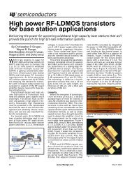
Figure 8. A block diagram <strong>of</strong> one potential RF data transmitter design using <strong>digital</strong> filters.<br />
56 www.rfdesign.com April 2002
eceiver is not known. Another design<br />
constraint is that the <strong>digital</strong> circuitry<br />
used to construct the <strong>digital</strong> filter will<br />
operate at a maximum rate <strong>of</strong> 50 MHz.<br />
Additionally, it has been given as part<br />
<strong>of</strong> the design requirement that the filter<br />
im<strong>pulse</strong> response span at least five<br />
symbol periods.<br />
In the absence <strong>of</strong> specific knowledge<br />
about timing jitter at the receiver, one<br />
is forced to assume the worst. This<br />
implies that a value <strong>of</strong> α = 1 be used to<br />
maximize the decay <strong>of</strong> the <strong>pulse</strong> tails.<br />
From Figure 2a, it can be seen that<br />
this corresponds to a single-sided b<strong>and</strong>width<br />
<strong>of</strong> 1/τ (1 MHz), which means that<br />
the medium over which the data are<br />
transmitted must be able to support a<br />
2 MHz b<strong>and</strong>width (the double-sided<br />
b<strong>and</strong>width <strong>of</strong> the raised cosine spectrum).<br />
If the medium cannot support<br />
2 MHz, then one must consider a<br />
means <strong>of</strong> squeezing more bits into the<br />
same b<strong>and</strong>width. This can be done by a<br />
variety <strong>of</strong> modulation schemes (QPSK,<br />
16-QAM, etc.). In this example, it is<br />
assumed that a b<strong>and</strong>width <strong>of</strong> 2 MHz is<br />
acceptable.<br />
Because it has been determined<br />
that α = 1, it is necessary to operate<br />
the filter at a sample rate <strong>of</strong> no less<br />
than twice the data rate (or two samples<br />
per symbol). However, to provide<br />
a more accurate spectral shape, one<br />
may choose to oversample by a factor<br />
<strong>of</strong> eight (i.e., eight samples/symbol).<br />
This means that the <strong>digital</strong> filter must<br />
operate at a rate <strong>of</strong> 8 MHz. This is<br />
well within the specified 50 MHz operating<br />
range <strong>of</strong> the <strong>digital</strong> circuitry, so<br />
the design is not in jeopardy.<br />
It has been given that the filter<br />
im<strong>pulse</strong> response be designed to span<br />
five symbols, so the filter must contain<br />
at least 40 taps (eight samples/symbol x<br />
five symbols = 40 samples). This will<br />
provide the required duration <strong>of</strong> the<br />
im<strong>pulse</strong> response. However, 41 taps will<br />
be chosen to avoid the half-symbol delay<br />
associated with an even number <strong>of</strong> taps.<br />
With α, τ, <strong>and</strong> the number <strong>of</strong> taps<br />
defined, Equation 2 can now be used to<br />
generate the filter taps. <strong>The</strong> value <strong>of</strong> t is<br />
determined at increments <strong>of</strong> 125 ns (the<br />
sampling period <strong>of</strong> the filter when operating<br />
at 8 MHz). <strong>The</strong> center <strong>of</strong> the<br />
im<strong>pulse</strong> response is given the value <strong>of</strong> t<br />
= 0. Thus, the first value <strong>of</strong> t is 20 samples<br />
prior, or t = -2.5 µs.<br />
How it all came together<br />
<strong>The</strong> author used a PC-based version<br />
<strong>of</strong> Mathcad to compute p(t) using the<br />
above information (see Appendix). Any<br />
suitable math program will do the job<br />
(MatLab, Excel, etc.). It turns out that<br />
because p(t) was computed at the filter<br />
sample points, the values <strong>of</strong> p(t) correspond<br />
one-to-one with h[n], the im<strong>pulse</strong><br />
response <strong>of</strong> the filter. <strong>The</strong> results,<br />
rounded to four decimal places, are listed<br />
in Table 1.<br />
Note the symmetry <strong>of</strong> the h(n) values<br />
about n = 0. This redundancy can be<br />
used to simplify the implementation <strong>of</strong><br />
the filter hardware. Because the filter is<br />
<strong>of</strong> the oversampling variety, further<br />
n h(n) n<br />
-20 0 20<br />
-19 -0.0022 19<br />
-18 0.0037 18<br />
-17 0.0031 17<br />
-16 0 16<br />
-15 0.0046 15<br />
-14 0.081 14<br />
-13 0.0072 13<br />
-12 0 12<br />
-11 0.0125 11<br />
-10 0.0234 10<br />
-9 0.0246 9<br />
-8 0 8<br />
-7 0.0624 7<br />
-6 0.1698 6<br />
-5 0.3201 5<br />
-4 0.5 4<br />
-3 0.686 3<br />
-2 0.8488 2<br />
-1 0.9603 1<br />
0 1 0<br />
Table 1. Im<strong>pulse</strong> response values for p(t) <strong>of</strong> the<br />
filter.<br />
hardware simplification can be gained<br />
by using a polyphase architecture.<br />
If the filter is designed with floating<br />
point multipliers <strong>and</strong> adders, then the<br />
design is essentially done.<br />
In the case <strong>of</strong> finite arithmetic, 10<br />
bits is probably the minimum acceptable<br />
resolution to h<strong>and</strong>le tap coefficients<br />
that span four decimal places.<br />
Formatted as twos-complement numbers,<br />
this will allow a range <strong>of</strong> –1.000<br />
to +0.998046875 with a resolution <strong>of</strong><br />
2 –10 (0.0009765625). This means that<br />
the multiply <strong>and</strong> add stages <strong>of</strong> the filter<br />
must be designed to h<strong>and</strong>le 10-bit<br />
words. Also, the coefficients should be<br />
scaled by some fractional value to<br />
avoid overflow conditions in the hardware.<br />
A generally accepted scale factor<br />
is given by:<br />
SF = [∑h(k) 2 ] –1/2 .<br />
In words, it is the reciprocal <strong>of</strong> the<br />
square root <strong>of</strong> the sum <strong>of</strong> the square <strong>of</strong><br />
each tap value. For the current example,<br />
the scale factor is: SF = 0.408249.<br />
After multiplying the h(n) by SF, the<br />
resulting values are then converted to<br />
10-bit words. Figure 7 shows the frequency<br />
responses <strong>of</strong> two versions <strong>of</strong><br />
the raised cosine <strong>pulse</strong>-<strong>shaping</strong> filter.<br />
One is a floating-point version <strong>of</strong> the<br />
filter with the coefficients rounded to<br />
four decimal places. <strong>The</strong> other is a<br />
scaled, 10-bit, finite-math version <strong>of</strong><br />
the filter. Both responses behave well<br />
in the passb<strong>and</strong>, but the floating-point<br />
version exhibits better out-<strong>of</strong>-b<strong>and</strong><br />
attenuation. Also shown for comparison’s<br />
sake is the passb<strong>and</strong> error relative<br />
to the ideal response (Equation 1).<br />
Note that both responses exhibit less<br />
than 0.2 dB error over a range <strong>of</strong><br />
about 90% <strong>of</strong> the passb<strong>and</strong>.<br />
<strong>The</strong> final frontier<br />
With an underst<strong>and</strong>ing <strong>of</strong> how to create<br />
<strong>digital</strong> <strong>pulse</strong> <strong>shaping</strong> filters, the RF<br />
engineer can take on a larger role in the<br />
design <strong>of</strong> <strong>digital</strong> transmission systems.<br />
This is especially true today with semiconductor<br />
manufacturers <strong>of</strong>fering highly<br />
integrated, high-speed, mixed-signal<br />
ICs. Figure 8 shows a detailed block<br />
diagram <strong>of</strong> a possible RF data transmitter<br />
design. <strong>The</strong> design is almost completely<br />
contained in two ICs (assuming<br />
a PC or other external device serves as<br />
the serial port controller).<br />
References<br />
[1] Gibson, J. D., “Principles <strong>of</strong> Analog<br />
<strong>and</strong> Digital Communications,” 2nd ed.,<br />
Prentice Hall, 1993.<br />
[2] Ifeachor, E. C., Jervis, B. W.,<br />
“Digital Signal Processing: A Practical<br />
Approach,” Addisson-Wesley<br />
Publishing Co., 1996.<br />
[3] <strong>The</strong> World Book Encyclopedia,<br />
Volume 13, World Book, Inc., 1994.<br />
58 www.rfdesign.com April 2002
About the author<br />
Ken Gentile graduated with honors from North Carolina State University<br />
where he received a B.S.E.E degree in 1996. Currently, he is a system design<br />
engineer at Analog Devices, Greensboro, NC. As a member <strong>of</strong> the Signal<br />
Synthesis Products group, he is responsible for the system level design <strong>and</strong> analysis<br />
<strong>of</strong> signal synthesis products. His specialties are analog circuit design <strong>and</strong> the<br />
application <strong>of</strong> <strong>digital</strong> signal processing techniques in communications systems. He<br />
can be reached at 336-605-4073 or by e-mail at ken.gentile@analog.com.<br />
RF Design www.rfdesign.com 61