Solving Problems in Dynamics and Vibrations Using MATLAB ...
Solving Problems in Dynamics and Vibrations Using MATLAB ...
Solving Problems in Dynamics and Vibrations Using MATLAB ...

Create successful ePaper yourself
Turn your PDF publications into a flip-book with our unique Google optimized e-Paper software.
21<br />
2. Simple Pendulum<br />
θ<br />
l<br />
m<br />
Example<br />
Compute <strong>and</strong> plot the l<strong>in</strong>ear response of a simple pendulum hav<strong>in</strong>g a mass of 10 grams <strong>and</strong> a<br />
length of 5 cms. The <strong>in</strong>itial conditions are θ (0) = 90° <strong>and</strong> θ (0) = 0<br />
Also compare the generated plot with the nonl<strong>in</strong>ear plot.<br />
Solution<br />
The differential equation of motion for the simple pendulum without any damp<strong>in</strong>g is given by<br />
.<br />
..<br />
g<br />
θ = ( − ) s<strong>in</strong>θ<br />
l<br />
If we consider the system to be l<strong>in</strong>ear, i.e., for small angles,<br />
s<strong>in</strong>θ =θ<br />
So the l<strong>in</strong>earized version of the above non-l<strong>in</strong>ear differential equation reduces to<br />
..<br />
g<br />
θ = ( − )θ<br />
l<br />
The above equation is a second order, constant-coefficient differential equation. In order to use<br />
<strong>MATLAB</strong> to solve it, we have to reduce it to two first order differential equations as <strong>MATLAB</strong><br />
uses a Runge-kutta method to solve differential equations, which is applicable only for first order<br />
differential equations.<br />
Let<br />
θ =<br />
y(1)<br />
.<br />
θ<br />
=<br />
y(2)