Solving Problems in Dynamics and Vibrations Using MATLAB ...

Solving Problems in Dynamics and Vibrations Using MATLAB
Parasuram Harihara
And
Dara W. Childs
Dept of Mechanical Engineering
Texas A & M University
College Station.

2
Contents
I. An Introduction to MATLAB…………………………………………………(3)
1. Spring-Mass-Damper system…………………………………………………(11)
2. Simple pendulum……………………………………………………………..(21)
3. Coulomb friction……………………………………………………..……….(26)
4. Trajectory motion with aerodynamic drag……………………………..……..(30)
5. Pendulum with aerodynamic and viscous damping……………………..……(34)
6. A half cylinder rolling on a horizontal plane……………………………..…..(38)
7. A bar supported by a cord…………………………………………………….(41)
8. Double pendulum……………………………………………………………..(50)
9. Frequency response of systems having more than one degree of freedom…...(56)
10. A three bar linkage problem…………………………………………………..(63)
11. Slider-Crank mechanism……………………………………………………....(70)
12. A bar supported by a wire and a horizontal plane……………………………..(77)
13. Two bar linkage assembly supported by a pivot joint and a horizontal plane…(84)
14. Valve Spring Model...........................................................................................(92)

3
An Introduction to MATLAB
Purpose of the Handout
This handout was developed to help you understand the basic features of MATLAB and also to
help you understand the use of some basic functions. This is not a comprehensive tutorial for
MATLAB. To learn more about a certain function, you should use the online help. For example,
if you want to know more about the function ‘solve’, then type the following command in the
command window at the prompt:
help solve
Introduction
MATLAB is a high performance language for technical computing. The name MATLAB stands
for matrix laboratory. Some of the typical uses of MATLAB are given below:
• Math and Computation
• Algorithm Development
• Modeling, Simulation and Prototyping
M-Files
Files that contain code in MATLAB language are called M-Files. You create a M-File using a
text editor and then use them as you would any other MATLAB function or command. But
before using the user defined functions always make sure that the ‘path’ is set to the current
directory. There are two kinds of M-Files:
• Scripts, which do not accept input arguments or return output arguments.
• Functions, which can accept input and output arguments.
When you invoke a script MATLAB simply executes the commands found in the file. For
example, create a file called ‘SumOfNumbers’ that contains these commands:
% To find the sum of first 10 natural numbers
n = 0;
i = 1;
for i=1:10;
n = n + i;
i = i + 1;
end
n
Go to the command window and set the path to the current directory. Then typing

4
SumOfNumbers
at the command prompt causes MATLAB to execute the commands in the M-File and print out
the value of the sum of the first 10 natural numbers.
Functions are dealt in detail later in the handout.
Matrices
Suppose you have to enter a 2x2 identity matrix in MATLAB. Type the following command in
the command window:
A=[1 0; 0 1]
MATLAB displays the matrix you just entered
A=
1 0
0 1
The basic conventions you need to follow are as follows:
• Separate the elements in the row with blanks or commas
• Use a semicolon, (;) to indicate the end of each row
• Surround the entire list of elements with square brackets, [].
There are many other ways of representing matrices, but the above-mentioned method is one of
the popularly used methods. To know more about the different types of representation, go
through the online help or the MATLAB user guide.
Suppose, you want to separate out the first column in the above matrix and use it for some other
calculation, then type the following in the MATLAB command window.
Y=A(:,1)
Here Y contains the elements of the first column. Y is a 2x1 matrix. Note that the colon in the
above expression indicates that MATLAB will consider all rows and ‘1’ indicates the first
column. Similarly if you want to separate the second row then type the following command
T=A(2,:)
Solving Linear Equations
Suppose for example, you have to solve the following linear equations for ‘x’ and ‘y’.

5
x + 2y
= 6
x − y = 0
There are two methods to solve the above-mentioned linear simultaneous equations.
The first method is to use matrix algebra and the second one is to use the MATLAB command
‘solve’.
Matrix Algebra
Representing the above two equations in the matrix form, we get
⎡1
⎢
⎣1
2 ⎤⎧x⎫
⎧6⎫
⎥⎨
⎬ = ⎨ ⎬
−1⎦⎩
y⎭
⎩0⎭
The above equation is in the form of
AX = B
where A is known as the coefficient matrix, X is called the variable matrix and B, the constant
matrix.
To solve for X, we find the inverse of the matrix A (provided the inverse exits) and then premultiply
the inverse to the matrix B i.e.,
X
=
A
−1
B
The MATLAB code for the above-mentioned operations is as shown below. Open a new M-File
and type in the following commands in the file.
% To solve two simultaneous linear equations.
A = [1 2;1 –1];
B = [6;0];
X = inv (A)*B
Before executing the program, always remember to set the path to the current directory. Note
that the first statement is preceded by a ‘%’ symbol. This symbol indicates that the statement
following the symbol is to be regarded as a comment statement. Also note that if you put a
semicolon ‘;’ after each statement, then the value of that statement is not printed in the command
window. Since we require MATLAB to print the value of ‘X’, the semicolon does not follow the
last statement.

6
Solve Command
The ‘solve’ command is a predefined function in MATLAB. The code for solving the above
equations using the ‘solve’ command is as shown. Open a new M-File and type the following
code.
% To solve the linear equations using the solve command
p = ‘x + 2*y = 6’;
q = ‘x – y = 0’;
[x,y] = solve(p,q)
Subs Command
This command is explained by means of the following example. Suppose you want to solve the
following linear equations:
x + 2y
= a + 6
x − y = a
Note that there are three unknown and only two equations. So we are required to solve for ‘x’
and ‘y’ in terms of ‘a’. To calculate the numerical values of ‘x’ and ‘y’ for different values of ‘a’,
we use the subs command.
The following MATLAB code is used to demonstrate the ‘subs’ command.
% To solve the linear equations using the subs command
p = ‘x + 2*y = a + 6’
q = ‘x – y = a’
[x,y] = solve(p,q)
a = 0;
[x] = subs(x)
[y] = subs(y)
Here the ‘solve’ command solves for the values of ‘x’ and ‘y’ in terms of ‘a’. Then ‘a’ is
assigned the value of ‘0’. Then we substitute the assigned value of ‘a’ in ‘x’ and ‘y’ to get the
numerical value.
Suppose a varies from 1 to 10 and we need to find the value of ‘x’ and ‘y’ for each value of ‘a’
then use the following code:
% To solve the linear equations using the subs command

7
p = ‘x + 2*y = a + 6’
q = ‘x – y = a’
[x,y] = solve(p,q)
i = 0;
for a = 1:10
t(i) = subs(x);
p(i) = subs(y);
i = i + 1 ;
end
In the above code t(i) and p(i) contains the values of ‘x’ and ‘y’ for different values of ‘a’
respectively.
Functions
Functions are M-Files that can accept input arguments and return output arguments. The name of
the M-File and the function should be the same. Functions operate on variables within their own
workspace, separate from the workspace you access at the MATLAB command prompt. The
following example explains the use of functions in more detail.
Define a new function called hyperbola in a new M-File.
Function y = twice(x)
y = 2*x;
Now in a new M-file plot ‘y’ with respect to ‘x’ for different values of ‘x’. The code is as shown
below
x = 1:10
y = twice(x)
plot(x,y)
Basically the function ‘twice’ takes the values of x, multiplies it by 2 and then stores each value
in y. The ‘plot’ function plots the values of ‘y’ with respect to ‘x’.
To learn more about the use of functions, go through the user guide.
Hold Command
HOLD ON holds the current plot and all axis properties so that subsequent graphing commands
add to the existing graph. HOLD OFF returns to the default mode whereby PLOT commands
erase the previous plots and reset all axis properties before drawing new plots.
One can also just use the ‘Hold’ command, which toggles the hold state. To use this command,
one should use a counter in connection with an ‘if’ loop; which first toggles the hold on state and

8
then the counter must be incremented such that, the flow of command does not enter the ‘if’
loop.
% Example to show the use of the hold command
counter = 0;
if (counter ==0)
hold;
end
counter = counter + 1;
Here the ‘hold’ command is executed only if the value of the counter is equal to zero. In this way
we can make sure that the plots are held. The drawback of this procedure is that we cannot toggle
the ‘hold’ to off.
Plotting Techniques
The plot function has different forms depending on the input arguments. For example, if y is a
vector, plot (y) produces a linear graph of the elements of y versus the index of the elements of y.
If you specify two vectors as arguments, plot (x,y) produces a graph of y versus x.
Whenever a plot is drawn, title’s and a label’s for the x axis and y axis are required. This is
achieved by using the following command.
To include a title for a plot use the following command
title (‘Title’)
For the x and y labels, use
xlabel(‘ label for the x-axis’)
ylabel(‘label for the y-axis’)
Always remember to plot the data with the grid lines. You can include the grid lines to your
current axes by including the following command in your code.
grid on
For more information about various other plotting techniques, type
help plot
in the command window.

9
Suppose one wants to change the color of the curve in the plot to magenta, then use the following
command
plot (x,y,’m’)
‘m’ is the color code for magenta. There are various other color codes like ‘r’ for red, ‘y’ for
yellow, ‘b’ for blue etc.
The following example makes use of the above-mentioned commands to plot two different data
in the same plot. The MATLAB code is given below.
x=0:0.1:10;
y1 = x.*2;
y2 = x.*3;
plot(x,y1)
hold on
plot(x,y2,'-.')
grid on
xlabel('x')
ylabel('y')
title('X Vs Y')
legend('y1','y2')
When you run the above code, you will get the following plot.
In order to save the plot as a JPEG file, click the file icon in the figure window and then click the
export command. In the ‘save as type’ option select ‘*.jpg’. In order to import the file in MS
word, go to ‘Insert’ icon and then select ‘Picture from file’ command.

10
Figure Command
Suppose you want to plot two different vectors in two different windows, use the “figure”
command. The example given below illustrates the use of the “figure” command.
% to illustrate the figure command
x=[1,2,3,4,5,6,7,8,9,10];
y=[12 23 4 5 65 67 89];
figure(1)
plot(x)
grid
title('plot of X')
figure(2)
plot(y)
grid
title('plot of Y')
The above code will plot the values of x and y in two different figure windows. If you want to
know more about the command type the following at the command prompt.
help figure

11
1. Spring Mass Damper System – Unforced Response
m
k
c
Example
Solve for five cycles, the response of an unforced system given by the equation
..
.
m x+ c x+
kx = 0
(1)
For ξ = 0.1; m = 1 kg; k = 100 N/m; x (0) = 0.02 m;
ẋ (0) = 0;
Solution
The above equation is a second order constant-coefficient differential equation. To solve this
equation we have to reduce it into two first order differential equations. This step is taken
because MATLAB uses a Runge-Kutta method to solve differential equations, which is valid
only for first order equations.
Let
.
x = v
(2)
From the above expression we see that
.
mv+
cv + kx = 0
so the equation (1) reduces to
.
− c k
v = [( ) v − ( ) x]
(3)
m m
We can see that the second order differential equation (1) has been reduced to two first order
differential equations (2) and (3).

12
For our convenience, put
x = y (1);
.
x = v = y(2);
Equations (2) and (3) reduce to
.
y (1) = y (2); (4)
.
y (2) = [(-c/m)*y (2) – (k/m)*y (1)]; (5)
To calculate the value of ‘c’, compare equation (1) with the following generalized equation.
..
.
2
x+ 2ξω
n
x+
ω
n
= 0
Equating the coefficients of the similar terms we have
c
m
= 2ξω
(6)
n
2 k
ω
n
=
(7)
m
Using the values of ‘m’ and ‘k’, calculate the different values of ‘c’ corresponding to each value
of ξ. Once the values of ‘c’ are known, equations (4) and (5) can be solved using MATLAB.
The problem should be solved for five cycles. In order to find the time interval, we first need to
determine the damped period of the system.
Natural frequency ω n = ( k / m)
= 10 rad/sec.
For ξ = 0.1
Damped natural frequency ω d = ω n 1− ξ 2
= 9.95 rad/sec.
Damped time period T d = 2π/ω d = 0.63 sec.
Therefore for five time cycles the interval should be 5 times the damped time period, i.e., 3.16
sec.

13
MATLAB Code
In order to apply the ODE45 or any other numerical integration procedure, a separate function
file must be generated to define equations (4) and (5). Actually, the right hand side of equations
(4) and (5) are what is stored in the file. The equations are written in the form of a vector.
The MATLAB code is given below.
function yp = unforced1(t,y)
yp = [y(2);(-((c/m)*y(2))-((k/m)*y(1)))]; (8)
Open a new M-file and write down the above two lines. The first line of the function file must
start with the word “function” and the file must be saved corresponding to the function call; i.e.,
in this case, the file is saved as unforced1.m. The derivatives are stored in the form of a vector.
This example problem has been solved for ξ = 0.1. We need to find the value of ‘c/m’ and ‘k/m’
so that the values can be substituted in equation (8). Substituting the values of ξ and ω n in
equations (6) and (7) the values of ‘c/m’ and ‘k/m’ can be found out. After finding the values,
substitute them into equation (8).
Now we need to write a code, which calls the above function and solves the differential
equation and plots the required result. First open another M-file and type the following code.
tspan=[0 4];
y0=[0.02;0];
[t,y]=ode45('unforced1',tspan,y0);
plot(t,y(:,1));
grid on
xlabel(‘time’)
ylabel(‘Displacement’)
title(‘Displacement Vs Time’)
hold on;
The ode45 command in the main body calls the function unforced1, which defines the systems
first order derivatives. The response is then plotted using the plot command. ‘tspan’ represents
the time interval and ‘y0’ represents the initial conditions for y(1) and y(2) which in turn
represent the displacement ‘x’ and the first derivative of ‘x’. In this example, the initial
conditions are taken as 0.02 m for ‘x’ and 0 m/sec for the first derivative of ‘x’.
MATLAB uses a default step value for the vector ‘tspan’. In order to change the step size use the
following code
tspan=0:0.001:4;
This tells MATLAB that the vector ‘tspan’ is from 0 to 4 with a step size of 0.001. This example
uses some arbitrary step size. If the step size is too small, the plot obtained will not be a smooth
curve. So it is always better to use relatively larger step size. But it also takes longer to simulate

14
programs with larger step size. So you have to decide which is the best step size you can use for
a given problem.
In order to solve for different values of ξ, calculate the values of ‘c/m’ for each value of ξ.
Substitute each value of ξ in the function file, which has the derivatives, save the file and then
run the main program to view the result. This process might be too tedious. The code can be
made more efficient by incorporating a ‘For loop’ for the various values of zeta.
In the above code ‘y(:,1) represents the displacement ‘x’. To plot the velocity, change the
variable in the plot command line to ‘y(:,2)’.
The plot is attached below

15
Assignment
Solve for six cycles the response of an unforced system given by
..
.
m x+ c x+
kx = 0
For ξ = {0, 0.1 0.25, 0.5, 0.75, 1.0}.
Take m = 5 kg; k = 1000 N/m; x(0) = 5 cms;
ẋ (0) = 0;
Develop a plot for the solutions corresponding to the seven ξ values and comment on the plots
obtained.
Note: When you save the M-File, make sure that the name of the file does not coincide with
any of the variables used in the MATLAB code.

16
Spring Mass Damper System – Forced Response
fsinωt
m
k
c
Example
Plot the response of a forced system given by the equation
..
.
m x+ c x+
kx = f sinω
t
(1)
For ξ = 0.1; m = 1 kg; k = 100 N/m; f = 100 N; ω = 2ω n ; x(0) = 2 cms;
ẋ (0) = 0.
Solution
The above equation is similar to the unforced system except that it has a forcing function. To
solve this equation we have to reduce it into two first order differential equations. Again, this
step is taken because MATLAB uses a Runge-Kutta method to solve differential equations,
which is valid only for first order equations.
Let
.
x = v
(2)
so the above equation reduces to
.
f c k
v = [( )sinω t − ( ) v − ( ) x]
(3)
m m m
We can see that the second order differential equation has been reduced to two first order
differential equations.

17
For our convenience, put
x = y (1);
.
x = v = y(2);
Equations (2) and (3) then reduce to
.
y (1) = y (2);
.
y (2) = [(f/m)*sin(ω * t) + (-c/m)*y (2) – (k/m)*y (1)];
Again, to calculate the value of ‘c’, compare equation (1) with the following generalized
equation
..
2
n
x+
2ξω x+
ω = f sinω
n
.
t
Equating the coefficients of the similar terms we have
c
= 2ξω
n
m
2 k
ω
n
=
m
Using the values of ‘m’ and ‘k’, calculate the different values of ‘c’ corresponding to each value
of ξ.
To find the time interval the simulation should run, we first need to find the damped time period.
Natural frequency ω n = ( k / m)
= 10 rad/sec.
For ξ = 0.1;
Damped natural frequency ω d = ω n 1− ξ 2
= 9.95 rad/sec.
Damped time period T d = 2π/ω d = 0.63 sec.
Therefore, for five time cycles the interval should be 5 times the damped time period, i.e., 3.16
sec. Since the plots should indicate both the transient and the steady state response, the time
interval will be increased.

18
MATLAB Code
The MATLAB code is similar to that written for the unforced response system, except that there
is an extra term in the derivative vector, which represents the force applied to the system.
The MATLAB code is given below.
function yp = forced(t,y)
yp = [y(2);(((f/m)*sin(ω n *t))-((c/m)*y(2))-((k/m)*y(1)))];
Again the problem is to be solved for ξ = 0.1. So, calculate the value of ‘c/m’, ‘k/m’ and ‘f/m’ by
following the procedure mentioned in the earlier example and then substitute these values into
the above expression. Save the file as ‘forced.m’.
The following code represents the main code, which calls the function and solves the differential
equations and plots the required result.
tspan=[0 5];
y0=[0.02;0];
[t,y]=ode45('forced',tspan,y0);
plot(t,y(:,1));
grid on
xlabel(‘time’)
ylabel(‘Displacement’)
title(‘Displacement Vs Time’)
hold on;
Again, ‘tspan’ represents the time interval and ‘y0’ represents the initial conditions for y(1) and
y(2) which in turn represent the displacement ‘x’ and the first derivative of ‘x’. In this example
the initial conditions are taken as 0.02 m for ‘x’ and 0 cm/sec for the first derivative of ‘x’. Again
the default step size of the vector ‘tspan’ can be changed accordingly as explained in the
previous example.
To solve for different values of ξ, calculate the values of ‘c/m’ for each value of ξ. Substitute
each value of ξ in the function file, which has the derivatives, save the file and then run the main
program to view the result.
In the above code ‘y(:,1) represents the displacement ‘x’. To plot the velocity, change the
variable in the plot command line to ‘y(:,2)’.
The plot is attached below.

20
Assignment
Plot the response of a forced system given by the equation
m x+
c x+
kx =
For ξ = {0, 0.1 0.25, 0.5, 0.75, 1.0}.
..
.
f
sinω
Take m = 5 kg; k = 1000 N/m; f = 50 N; ω = 4ω n , x(0) = 5 cms;
t
ẋ (0) = 0.
Develop a plot for the solutions corresponding to the seven ξ values and comment on the plots
obtained.

21
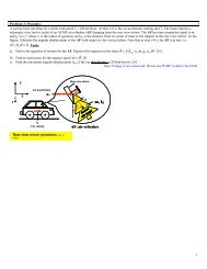
2. Simple Pendulum
θ
l
m
Example
Compute and plot the linear response of a simple pendulum having a mass of 10 grams and a
length of 5 cms. The initial conditions are θ (0) = 90° and θ (0) = 0
Also compare the generated plot with the nonlinear plot.
Solution
The differential equation of motion for the simple pendulum without any damping is given by
.
..
g
θ = ( − ) sinθ
l
If we consider the system to be linear, i.e., for small angles,
sinθ =θ
So the linearized version of the above non-linear differential equation reduces to
..
g
θ = ( − )θ
l
The above equation is a second order, constant-coefficient differential equation. In order to use
MATLAB to solve it, we have to reduce it to two first order differential equations as MATLAB
uses a Runge-kutta method to solve differential equations, which is applicable only for first order
differential equations.
Let
θ =
y(1)
.
θ
=
y(2)

22
When the values of ‘theta’ and the first derivative of ‘theta’ are substituted in the second order
linearized differential equation, we get the following two first order differential equation:
For a nonlinear system,
sinθ ≠θ
ẏ(
1 ) = y( 2 )
The second order non-linear differential equation reduces to the following, two first order
differential equation:
.
.
y (1) = y(2)
y(2)
= ( −g / l)sin(
y(1))
MATLAB Code
The MATLAB code is written following the procedure adopted to solve the spring-mass-damper
system. For the linear case the function file is saved as ‘linear.m’.
function yp = linear(t,y)
yp = [y(2);((-g/l) *(y(1)))];
In this example, the value of ‘l’ is chosen to be 5 cms. So the value of ‘g/l’ turns out to be –196.2
per square second. Note that since the mass and the length are expressed in grams and
centimeters respectively, the value of the acceleration due to gravity ‘g’ is taken to be 981 cms
per square second. Substitute this value in the above MATLAB code.
For the nonlinear case, open a new M-file to write a separate function file for the nonlinear
differential equation. In this case the function file is saved as ‘nonlinear.m’.
function yp = nonlinear(t,y)
yp = [y(2);((-g/l) *sin(y(1)))];
The main code should be written in a separate M-file, which will actually call the above function
files, solve the derivatives stored in them and plot the required result.
tspan = [0 5];
y0 = [1.57;0];
[t,y] = ode45('linear',tspan,y0)
plot(t,y(:,1))
grid on;
xlabel(‘Time’)
ylabel(‘Theta’)
title(‘Theta Vs Time’)
hold on;

23
‘tspan’ represents the time interval and ‘y0’ represents the initial condition. Note that the value
of θ in the initial conditions must be expressed in radians.
Now run the code for the linearized version of the simple pendulum. A plot of ‘theta’ versus
‘time’ will be obtained. The ‘hold’ command in the code freezes the plot obtained. This
command is used so that the nonlinear version can also be plotted in the same graph. After
running the program for the linear version, change the name of the function in the third line of
the main code from ‘linear’ to ‘nonlinear’. By doing this, the Ode45 command will now solve
the nonlinear differential equations and plot the result in the same graph. To differentiate
between the linear and the non-linear curve, use a different line style.
The plots of the responses are attached. From the plots we can see that the time period for the
non linear equation is greater than that of the linear equation.
To plot the angular velocity with respect to ‘time’ change the variable in the plot command line
in the main code from ‘y(:,1)’ to ‘y(:,2)’. This is done because initially we assigned y(1) to
‘theta’ and y(2) to the first derivative of ‘theta’.

25
Assignment
a) Compute and plot the response of a simple pendulum with viscous damping whose
equation of motion is given by
ml
2
..
.
θ + cθ
+ mglθ
= 0
Compute the value of the damping coefficients for ξ = 0.1.The initial conditions are
θ (0) = {15°, 30°, 45°, 60°, 90°} and θ (0) = 0 . M = 10 g ; l = 5 cms.
b) Compare the generated plot with Non-linear plot for each value of θ(0).
What do you infer from the plots obtained?
.
c) Plot the natural frequency of the nonlinear solution versus initial condition θ(0).
(Note: Plot the linear and the nonlinear curve in the same plot. Remember to convert the initial
values of theta given in degrees, to radians.)
Also make sure that the difference between the linear and the non-linear responses can be clearly
seen from the plot. If necessary use the zoom feature in order to show the difference.

26
3. Coulomb Friction
Example
Solve the following differential equation for θ ≥ 0 .
2
θ ..
.
g
2
(1 + sinθ
) + µ cosθ θ = [cosθ
(1 − µ ) − µ
d
d
l
d
d
µ
d
µ ={0, 0.1,0.2}; l = 0. 25m
. θ (0) = 0; θ(0)
= 0
Solution
.
.
sinθ
]
As explained earlier, to solve the above differential equation by MATLAB, reduce it into two
first order differential equations.
Let θ = y(1)
.
θ = y(2)
The above equation reduces to
.
y (1) = y(2)
.
g
2
y(2)
=
{cos( y(1))[1
− µ
d
] − µ
d
sin( y(1))}
−
l(1
+ µ sin( y(1)))
l(1
+ µ
d
d
1
{ µ
sin( y(1)))
d
cos( y(1))(
y(2)^2)}
MATLAB Code
A M-file must be written to store the derivatives. In this case the file is saved as ‘coulomb.m’.
function yp =coulomb(t,y)
g=9.81;
mu=0;
l=0.25;
k1=1+mu*sin(y(1));
k2=mu*cos(y(1))*(y(2)^2);
k3=cos(y(1))*(1-mu^2);
k4=mu*sin(y(1));
yp=[y(2);((g/l)*((k3-k4)/k1)-(k2/k1))]
Type the following code in a new M-file.

27
tspan=[0 2]
y0=[0;0]
[t,y]=ode45('coulomb',tspan,y0)
plot(t,y(:,1))
grid
xlabel(‘Time’)
ylabel(‘Theta’)
title(‘Theta Vs Time’)
hold on;
This main file calls the function ‘coulomb.m ’ to solve the differential equations. ‘Tspan’
represents the time interval and ‘y0’ represents the initial condition vector. To plot the results for
different values of µ, change the value of µ in the function file, save it and then run the main
code.
The vector ‘y(:,1)’ represents the values of theta at the various time instants and the vector
‘y(:,2)’ gives the values of the angular velocities. To plot the angular velocity, change the
variable in the plot command line in the main code from ‘y (:,1)’ to ‘y(:,2)’. Also plot the angular
velocity with respect to theta.
The plots are attached. From the plots it can be seen that by increasing the value of the coulomb
π
damping constant the system takes more time to reach θ= and the maximum value of the
2
angular velocity also decreases.

29
Assignment
.
Solve the following differential equation for θ ≥ 0 .
2
θ ..
.
g
2
(1 + sinθ
) + µ cosθ θ = [cosθ
(1 − µ ) − µ
d
d
l
d
d
µ
d
sinθ
]
µ ={0, 0.05,0.1,0.15,0.2}; l = 0. 5m
. θ (0) = π / 2; θ(0)
= 0
a) Plot the maximum value of angular velocity and maximum value of theta with respect
to µ
.
b) Is the differential equation valid for θ < 0 . If not, what is the correct equation?
c) Analytically confirm the angular velocity predictions for µ = 0.0 and µ = 0.2.
d) Comment on the results obtained.
.

30
4. Trajectory Motion with Aerodynamic Drag
Example
Solve the following differential equations for c
d
={0.1, 0.3,0.5} N/m.
..
m
d
.
.
2
2
x+ c x(
x + y
..
.
.
.
)
(1/ 2)
= 0
2 2 (1/ 2)
m y+
cd y(
x + y ) = −w
.
.
.
m = 10 kg. x(0)
= 100 m/s; y(0)
= 10 m/s; x(0) = 0; y(0) = 0.
Solution
As explained earlier, to solve the above two differential equations, we have to reduce each of
them into two first order differential equations.
So Let
x =
.
x =
y =
.
y =
y(1)
y(2)
y(3)
y(4)
The above equations reduce to the following first order differential equations.
.
y (1) = y(2)
.
cd
2
y( 2) = ( − ) * y(2) *[ y(2)
+ y
.
m
y (3) = y(4)
(4)
.
cd
2
( 4) = ( ) − ( ) * y(4) *[ y(2)
+ y
y
− w
m
m
2
]
1
2
(4)
2
]
1
2

31
MATLAB Code
Type the following code in a separate m-file. As mentioned earlier, the system derivatives must
be written in a separate m-file. Since the name of the function is ‘airdrag’, save the m-file as
‘airdrag.m’ in the current directory.
function yp = airdrag(t,y)
m = 10;
cd = 0.2;
g = 9.81;
w = m*g;
yp = zeros(4,1);
yp(1) = y(2);
yp(2) = ((-cd/m)*y(2)*(y(2)^2+y(4)^2)^(0.5));
yp(3) = y(4);
yp(4) = ((-w/m)-(cd/m)*y(4)*(y(2)^2+y(4)^2)^(0.5));
Open a new m-file and type the following code for the main program. This program calls the
function ‘airdrag.m’ in order to solve the differential equations. Again ‘tspan’ represents the time
interval and ‘y0’ represents the initial condition vector. The plots have to be drawn between the
displacement in the x direction and the displacement in the y direction. Refer to the handout
‘Introduction to MATLAB’ for the explanation about using the ‘hold’ command with the help of
a ‘counter’ variable.
tspan=[0 5];
y0=[0;100;0;10]
[t,y]=ode45('airdrag',tspan,y0);
plot(y(:,1),y(:,3))
grid
xlabel(‘X-Displacement’)
ylabel(‘Y-Displacement’)
title(‘X vs Y Displacement’)
hold on;
It can be seen from the plots that as the coefficient of the aerodynamic drag is increased the
maximum value of the displacement in the y direction decreases. The value of the displacement
in the x direction, for which the displacement in the y direction is maximum, also decreases.
Here the plots have been zoomed to the current version so that the difference in the curves could
be seen clearly.

33
Assignment
Solve the following differential equations for c
d
={0.0, 0.1,0.2,0.3} N/m.
..
m
d
.
.
2
2
x+ c x(
x + y
..
.
.
.
)
(1/ 2)
= 0
2 2 (1/ 2)
m y+
cd y(
x + y ) = −w
.
.
.
m = 5 kg. x(0)
= 10 m/s; y(0)
= 200 m/s; x(0) = 0; y(0) = 0.
a) Plot separately the maximum range and the maximum elevation with respect the
damping coefficient, C d.
b) Analytically confirm the results for C d = 0.
c) Comment on the results obtained.

34
5. Pendulum with Aerodynamic and Viscous Damping
Example
Solve the following non-linear differential equation with aerodynamic damping
..
2
g C
. .
a
θ + sinθ
+ θ sgn( θ)
= 0
(1)
l ml
and compare it with the following linearized differential equation with viscous damping
.. .
cd g
θ + θ + θ = 0
(2)
m l
.
m = 10 g; l = 5 cms; C a = C d = 14 ; θ (0) = 1.57; θ(0)
= 0.
(Note: The initial value of theta is given in radians.)
Solution
As mentioned earlier, to solve the above differential equations, convert them into two first order
differential equations.
Let
θ
.
θ
=
=
y(1)
y(2)
Equation (2) becomes
.
y (1) = y(2)
(3)
.
g cd
y(2)
= ( − ) *( y(1))
− ( ) *( y(2))
(4)
l
m
Similarly equation (1) becomes
.
y (1) = y(2)
(5)
.
g cd
y(2)
= ( − ) *sin( y(1))
− ( ) *( y(2)^2)sgn(
y(2))
(6)
l
ml
MATLAB Code
In this example, we are required to solve two separate problems, i.e., a pendulum with
aerodynamic drag and a pendulum with viscous damping. So, we have to write two separate M-
files, ‘pendulum1.m’, which contains the derivatives of the problem with aerodynamic drag and
‘pendulum2.m’, which contains the derivatives of the problem with viscous damping.

35
Open a new m-file and type the following code which contains equations (5) and (6). Note that
the derivatives are represented in the form of a vector. Also note that the signum function, ‘sgn’
has to be written as ‘sign’ in MATLAB.
function yp = pendulum1(t,y)
m=10;
g=981;
l=5;
Ca=14;
yp=[y(2);((-g/l)*sin(y(1))-Ca/(m*l)*(y(2)^2)*sign(y(2)))];
In a new m-file type in the following main program, which calls the function, named
‘pendulum1.m’ and solves the non-linear differential equation and plots it.
tspan=[0 10];
y0=[1.57;0]
[t,y]=ode45('pendulum1',tspan,y0);
plot(t,y(:,1));grid
xlabel(‘Time’)
ylabel(‘Theta’)
title(‘Theta Vs Time’)
hold on;
Open a new m-file type the following code. This file contains equations (3) and (4).
function yp = pendulum2(t,y)
m=10;
g=981;
l=5;
Ca=14;
yp=[y(2);((-g/l)*(y(1))-(Ca/m)*(y(2)))];
In a new m-file type the following main program. This code calls the function and solves the
linearized differential equation and plots it.
tspan=[0 10];
y0=[1.57;0]
[t,y]=ode45('pendulum2',tspan,y0);
plot(t,y(:,1));grid
xlabel(‘Time’)
ylabel(‘Theta’)
title(‘Theta Vs Time’)
hold on;
As mentioned in the earlier examples, ‘tspan’ represents the time interval and ‘y0’ represents the
initial condition vector. The vector ‘y(:,1)’ gives the values of theta at the various time instants

36
and the vector ‘y(:,2)’ gives the values of the angular velocity. To plot the angular velocity,
change the variable ‘y(:,1)’ in the plot command line to ‘y(:,2)’.
From the plots it can be seen that, quadratic damping causes a rapid initial amplitude reduction
but is less effective as time increases and amplitude decreases. Whereas, linear damping is less
effective initially but is more effective as time increases.

37
Assignment
a) Solve the following non-linear differential equation with aerodynamic damping
..
2
g C
. .
a
θ + sinθ
+ θ sgn( θ)
= 0
(1)
l ml
and compare it with the following linearized differential equation with viscous damping
.. .
cd g
θ + θ + θ = 0
(2)
m l
.
m = 5 g; l = 10 cms; C a = C d = 140; θ (0) = 0.5233; θ(0)
= 0.
Show the results in the same plot.
b) Comment on the results obtained. Assuming a harmonic motion, i.e., θ = A cos(ω n t), for what
amplitude ‘A’, are the linear and the non-linear damping moments equal? Also confirm the result
from the plot obtained.

38
6. A Half Cylinder rolling on a Horizontal Plane
Example
The general governing differential equation of motion of the above problem is
2
2
3mr
..
.
( − 2mer
sin β ) β − mer cos β β = wecos
β . (1)
2
4r
Solve the above differential equation for m = 5 Kg; e = m; r = 0.1 m.
3π
Solution
To solve the differential equation, convert the equation into two first order differential equation.
With
β
.
β
=
=
y(1);
y(2);
Equation (1) reduces to the following equations
.
y(1)
= y(2);
.
[ wecos(
y(1))
+ mer cos( y(1))(
y(2)^2)]
y(2)
=
[1.5mr^2
− 2mer
sin( y(1))]
MATLAB Code
The function file ‘tofro.m’ contains the systems derivatives in the form of a vector.
function yp = tofro(t,y)
m=5;
r=0.1;
e=(4*r)/(3*pi);
g=9.81;
yp=[y(2);((m*g)*e*cos(y(1))+m*e*r*cos(y(1))*(y(2)^2))/(1.5*m*r*r
-2*m*e*r*sin(y(1)))]
The main code, which is given below calls the function ‘tofro.m’, which contains the system
differential equation and plots the displacement with respect to time. Since there is no damping
present, the plot resembles a sinusoid of constant amplitude.
tspan=[0 4];

39
y0=[0.5233;0];
[t,y]=ode45('tofro',tspan,y0);
plot(t,y(:,1));grid
xlabel(‘Time’)
ylabel(‘Beta’)
title(‘Beta Vs Time’)
The plot is attached below.

40
Assignment
4r
a) Solve the differential equation given in the example for m = 10 Kg; e = m; r = 0.2 m. Plot
3π
‘β’ with respect to time. Compare the result with that obtained in the example and comment on
the result.
b) Determine the equilibrium value of ‘β’.
c) Linearize the differential equation for small motion about the equilibrium value and determine
the natural frequency for the small motion. Also plot the value of the ‘β’ with respect to time.
Note that for plotting the value of ‘β’, you have to solve the linearized differential equation.
d) Compare the natural frequency of the linearized model to that produced by the non- linear
model.

41
7. A bar supported by a cord
Derive the governing differential equation of motion of a swinging bar supported at its ends by a
cord. Calculate the eigen values and the eigen vectors. Solve the derived differential equation
and plot the initial response of the system for the following initial conditions:
a) Arbitrary initial condition
b) Initial condition vector proportional to the eigen vector.
Choose l 1 = 1m; l 2 = 1m; m 2 = 5Kg
φ l 1
θ
l 2 , m 2
The differential equations of motion for the above system when represented in a matrix form is
⎡
⎢
⎢
⎢m2l1l
⎢⎣
2
m l
2 1
cos( θ
2
−φ)
m2l2
cos( θ
2
2
m2l2
3
⎧
−φ)
⎤
.. ⎪
⎥ −
⎪
⎧
⎪
⎫ w
φ ⎪
⎥⎨
.. ⎬ = ⎨
⎥⎪⎩
θ ⎪⎭ ⎪−
w2l
⎥⎦
⎪
⎩
2
2
.
2 ⎫
m2l2
θ sin( θ − φ)
sinφ
+
⎪
2 ⎪
. 2 ⎬
sinθ
+ m sin( − ) ⎪
2l1l2
φ θ φ
⎪
2
⎭
Eliminating the second order terms in the above equation gives the linear equation
⎡
⎢ m2l1
⎢
⎢m2l1l
⎢⎣
2
2
2
m2l2l1
⎤
..
1
2
⎥ ⎡
⎪
⎧
⎪
⎫ l w
φ
⎢
2 ⎥⎨
.. ⎬ +
m2l2
⎥ ⎢ 0
⎪⎩ ϑ⎪⎭
⎣
3 ⎥⎦
2
0
w2l
2
2
⎤
⎧φ
⎫
⎥⎨
⎬ = 0
⎥
⎦
⎩θ
⎭
Note that the inertia matrix has been made symmetric via a multiplication of the first row by l 1 .

42
MATLAB Code
To find the eigen values and the eigen vectors
To find the eigen values and the eigen vectors, the linearized version of the model is used. The
mass of the bar was considered to be 5 Kg and the length of the cord and the bar to be 1m. The
MATLAB code is given below.
% to find the eigen values and the eigen vectors.
l1=1;
l2=1;
m2=5;
g=9.81;
w2=m2*g;
M=[m2*l1^2 (m2*l1*l2)/2;(m2*l1*l2)/2 (m2*l1^2)/3];
K=[l1*w2 0;0 (w2*l2)/2];
[v,d]=eig(K,M)
The columns ‘v’ represent the eigen vectors corresponding to each eigen value ‘d’.
‘M’ represents the inertia matrix and ‘K’ represents the stiffness matrix. The square root of the
eigen values gives the natural frequencies of the system.
The eigen values were found to be 6.2892 and 91.8108 and the corresponding eigen vectors were
⎧0.6661⎫
⎧− 0.4885⎫
⎨ ⎬and
⎨ ⎬respectively.
⎩0.7458⎭
⎩ 0.8726 ⎭
Initial response
To plot the initial response of the system the original nonlinear differential equation has to be
used. Moreover the second order differential equation has to be converted into a vector of first
φ = y(1);
.
φ = y(2);
θ = y(3);
.
θ = y(4);
order differential equation. This step is done by following the procedure given below.
Substituting the above relations in the original nonlinear differential equation, we get the
following nonlinear first order differential equation, which when represented in matrix form is
. ⎧
y(2)
⎫
⎡1
0 0 0 ⎤⎧
⎫
⎪
⎪
− ⎪
⎢
− ⎪
(1)
2
m ⎥
sin( (3) (1))
2l2
cos( y(3)
y(1))
y
m2l2θ
y y
⎪−
sin +
⎪ ⎪
⎪
⎢0
m 0
.
2l
w2
φ
1
2 ⎥ y(2)
2
⎢0
0 1 0 ⎥⎨
. ⎬ = ⎨
y(4)
⎬
⎢
⎢0
⎢⎣
m2l1l
2
cos( y(3)
− y(1))
2
0
m2l
3
2
2
⎥⎪y(3)
⎪
⎥⎪
. ⎪
⎥⎦
⎩y(4)
⎭
⎪
⎪
⎪
⎩
− w l
2 2
sinθ
+ m2l1l
2
. 2
2
φ
sin( θ −φ)
⎪
⎪
⎪
⎭

43
MATLAB Code
In this type of a problem where the inertia matrix (mass matrix) is a function of the states or the
variables, a separate M-file has to be written which incorporates a switch/case programming with
a flag case of ‘mass’.
For example if the differential equation is of the form,
M (t, y) *y’ (t)=F (t, y),
then the right hand side of the above equation has to be stored in a separate m-file called ‘F.m’.
Similarly the inertia matrix (mass matrix) should also be stored in a separate m-file named
‘M.m’. So, when the flag is set to the default, the function ‘F.m’ is called and later when the flag
is set to ‘mass’ the function ‘M.m’ is called.
The code with the switch/case is given below. Note that it is a function file and should be saved
as ‘indmot_ode.m’ in the current directory.
function varargout=indmot_ode(t,y,flag)
switch flag
case ''
%no input flag
varargout{1}=FF(t,y);
case 'mass'
%flag of mass calls mass.m
varargout{1}=MM(t,y);
otherwise
error(['unknown flag ''' flag '''.']);
end
To store the right hand side of the original matrix form of differential equation, a separate
function file must be written as shown below. Note that the name of the function is ‘FF’, so this
file must be saved as ‘FF.m’.
%the following function contains the right hand side of the
%differential equation of the form
%M(t,y)*y'=F(t,y)
%i.e. it contains F(t,y).it is also stored in a separate file
named, FF.m.
function yp=FF(t,y)
l1=1;
l2=1;
m2=5;
g=9.81;
w2=m2*g;
yp=zeros(4,1);

44
yp(1)=y(2);
yp(2)=-w2*sin(y(1))+ (m2*l2/2)*(y(4)^2)*sin(y(3)-y(1));
yp(3)=y(4);
yp(4)=(-w2*l2*sin(y(3)))/2+(m2*l1*l2/2)*(y(2)^2)*sin(y(3)-y(1));
Similarly, to store the mass matrix a separate function file is written which is stored as ‘MM.m’.
% the following function contains the mass matrix.
%it is separately stored in a file named, MM.m
function n = MM(t,y)
l1=1;
l2=1;
m2=5;
g=9.81;
w2=m2*g;
n1=[1 0 0 0];
n2=[0 m2*l1 0 (m2*l2/2)*cos(y(3)-y(1))];
n3=[0 0 1 0];
n4=[0 (m2*l1*l2/2)*cos(y(3)-y(1)) 0 m2*l2*l2/3];
n=[n1;n2;n3;n4];
To plot the response, the main file should call the function ‘indmot_ode.m’, which has the
switch/case programming which in turn calls the corresponding functions depending on the value
of the flag. For the main file to recognize the inertia matrix, the MATLAB command ODESET is
used to set the mass to ‘M (t, y)’.
This MATLAB code for the main file should be written in the same M-file, following the code to
solve for the eigen values and eigen vectors.

45
tspan=[0 30]
y0=[0.5233;0;1.0467;0] % Arbitrary Initial condition
x01=[v(1,1);0;v(2,1);0] % Low Frequency mode initial
Condition
x02=[v(1,2);0;v(2,2);0] % High frequency mode initial
Condition
options=odeset('mass','M(t,y)')
[t,y]=ode113('indmot_ode',tspan,y0,options)
subplot(2,1,1)
plot(t,y(:,1))
grid
xlabel('Time')
ylabel('phi')
subplot(2,1,2)
plot(t,y(:,3))
grid
xlabel('Time')
ylabel('Theta')
The above code plots the values of ‘theta’ and ‘phi’ with respect to time for the arbitrary initial
condition case. To plot for the initial condition case where the initial conditions are proportional
to the eigen vectors, change the variable ‘y0’ in line 6 of the code to first ‘x01’ and then to ‘x02’.
Notice the command “ subplot”.
subplot(m,n,p), breaks the Figure window into an m-by-n matrix of small axes and selects the p-
th axes for the current plot. The axes are counted along the top row of the Figure window, then
thesecond row, etc. For example,
subplot(2,1,1), plot(income)
subplot(2,1,2), plot(outgo)
plots “income” on the top half of the window and “outgo” on the bottom half.
From the plots it can be observed that: a) For initial condition vector that is proportional to the
eigen vectors, the response amplitudes are harmonic at their corresponding natural frequency. b)
For an arbitrary initial condition, we get a coupled response displaying response at both the
natural frequencies. The plots are attached below

49
Assignment
Solve the above-derived differential equation and plot the initial response of the system for the
following initial conditions:
a) Arbitrary initial condition
b) Initial condition vector proportional to the eigen vector.
Choose l1=2m; l2=4m; m2=10Kg.
Compare the results obtained from that of the example and comment on the plots obtained.

50
8. Double Pendulum
Derive the governing differential equation of motion of a double pendulum. Solve the derived
differential equation and plot the values of θ 1 and θ 2 with respect to time.
Choose l 1 = 1m; l 2 = 1m; m 1 = m 2 = 5Kg. The initial conditions for θ 1 and θ 2 are 0.5233 and
0.5233 radians respectively.
θ 1 l 1 , m 1
θ 2 l 2 , m 2
Solution
When represented in a matrix form, the differential equations of motion for the above system is
⎡ ( m2
+ m1
) l1
⎢
⎣m2l1
cos( θ
2
−θ1)
m
2
l
2
cos( θ
m
2
l
2
2
−θ
1
..
) ⎤
⎧
⎪θ
⎥⎨
..
⎦⎪⎩
θ
1
2
⎧
. 2
⎫
⎪ ⎪−
( w1
+ w2
)sinθ1
+ m2l2
θ
2
sin( θ
2
−θ
⎬ = ⎨
.
2
⎪⎭ ⎪
⎩ − w2
sinθ
2
− m1l1
θ 1 sin( θ
2
−θ1)
1)
⎫
⎪
⎬
⎪
⎭
MATLAB Code
These coupled second order differential equations must be converted into a vector of first order
differential equation. This step is done by the following substitutions.
θ
θ
θ
θ
1
.
1
2
.
2
= y(1);
= y(2);
= y(3);
= y(4);
Substituting the above relations in the original nonlinear differential equation, we get the
following first order differential equations,
.
⎧ ⎫
⎡1
0 0 0 ⎤ ⎧
⎫
⎪
y(1)
y(2)
⎪
⎢
⎥
. ⎪
. 2 ⎪
⎪ ⎪
⎢
0 ( m2
+ m1
) l1
0 m2l2
cos( θ
2
−θ1)
⎥ y(2)
⎪−
( w1
+ w2
)sinθ1
+ m2l2
θ
2
sin( θ
2
−θ1)
⎪
⎨ . ⎬ = ⎨
⎬
⎢0
0 1 0 ⎥
⎪ ⎪ ⎪
(4)
⎪
⎢
⎥
y(3)
y
.
⎣0
m cos( − ) 0
⎦
⎪ . ⎪ ⎪
2
⎪
2l1
θ
2
θ1
m2l2
⎩ − sin − sin( − )
⎩y(4)
w2
θ
2
m1l1
θ 1 θ
2
θ1
⎭
⎭

51
In this type of a problem where the coefficient matrix is a function of the states or the variables, a
separate M-file must be written which incorporates a switch/case programming with a flag case
of ‘mass’.
For example if the differential equation is of the form,
M (t, y) *y’ (t) = F (t, y),
then the right hand side of the above equation has to be stored in a separate m-file called ‘F.m’.
Similarly the coefficient matrix should be stored in a separate m-file named ‘M.m’. So, when the
flag is set to the default, the function ‘F.m’ is called and later when the flag is set to ‘mass’ the
function ‘M.m’ is called.
The code with the switch/case is given below. Note that it is a function file and should be saved
as ‘indmot_ode.m’ in the current directory.
function varargout=indmot_ode(t,y,flag)
switch flag
case ''
%no input flag
varargout{1}=pend(t,y);
case 'mass'
%flag of mass calls mass.m
varargout{1}=mass(t,y);
otherwise
error(['unknown flag ''' flag '''.']);
end
To store the right hand side of the state variable matrix form of the model, a separate function
file must be written as shown below. Note that the name of the function is ‘FF’, so this file must
be saved as ‘FF.m’.
%the following function contains the right hand side of the
%differential equation of the form
%M(t,y)*y'=F(t,y)
%i.e. it contains F(t,y).it is also stored in a separate file
named, pend.m.
function yp= pend(t,y)
M1=5;
M2=5;
g=9.81;
l1=1;
l2=1;
w2=M2*9.81;
w1=M1*9.81;
yp=zeros(4,1);

52
yp(1)=y(2);
yp(2)=-(w1+w2)*sin(y(1))+M2*l2*(y(4)^2)*sin(y(3)-y(1));
yp(3)=y(4);
yp(4)=-w2*sin(y(3))-M2*l1*(y(2)^2)*sin(y(3)-y(1));
Similarly, to store the coefficient matrix a separate function file is written which is stored as
‘MM.m’.
% the following function contains the mass matrix.
%it is separately stored in a file named, mass.m
function m = mass(t,y)
M1=5;
M2=5;
g=9.81;
l1=1;
l2=1;
m1=[1 0 0 0];
m2=[0 (M1+M2)*l1 0 M2*l2*cos(y(3)-y(1))];
m3=[0 0 1 0];
m4=[0 M2*l1*cos(y(3)-y(1)) 0 M2*l2];
m=[m1;m2;m3;m4];
To plot the response, the main file should call the function ‘indmot_ode.m’, which has the
switch/case programming which in turn calls the corresponding functions depending on the value
of the flag. For the main file to recognize the coefficient matrix, the MATLAB command
ODESET is used to set the mass to ‘M (t, y)’.
This MATLAB code for the main file should be written in the same M-file, following the code to
solve for the eigen values and eigen vectors.
% this is the main file, which calls the equations and solves
using ode113.
%it then plots the first variable.
tspan=[0 10]
y0=[0.5233;0;0.5233;0]
options=odeset('mass','M(t,y)')
[t,y]=ode113('indmot_ode',tspan,y0,options)
subplot(2,1,1)
plot(t,y(:,1))
grid
xlabel('Time')
ylabel('Theta1')

53
subplot(2,1,2)
plot(t,y(:,3))
grid
xlabel('Time')
ylabel('Theta2')
For help regarding ‘subplot’ refer to the previous example or you can look in the online help in
MATLAB by typing the following statement at the command prompt.
help subplot
The plot has been attached.

55
Assignment
1.) For the double pendulum problem, calculate the eigen values and eigen vectors.
2.) Solve the above-derived differential equation and plot the initial response of the system for
the following initial conditions:
a) Arbitrary initial condition
b) Initial condition vector proportional to both eigen vectors.
Choose l 1 = 2m; l 2 = 4m; m 1 = m 2 = 10Kg.
What do you infer from the plots?

56
9. Frequency response of systems having more than one degree of freedom
Example
Consider the following system as shown in the figure below. Derive the governing differential
equation of motion and plot the amplitude and the phase of the masses m 1 and m 2 with respect to
the frequency. Choose m 1 = 1Kg; m 2 = 2Kg; k 1 = k 2 = 1N/m; c 1 = c 2 = 0.001 N sec/m. The
amplitude of the excitation force vector is 1 N.
f 1 f 2
K 1 K 2
C 1 M 1 C 2 M 2
Solution
The governing differential equation of motion for the above system when written in matrix form
is given by
⎡m
⎢
⎣ 0
1
..
0 ⎤
⎧
⎪x
⎥⎨
..
m2
⎦⎪⎩
x
⎫
⎪ ⎡(
c1
+ c2
)
⎬ + ⎢
⎣ − c2
⎪⎭
1
2
− c
c
2
2
.
⎤
⎧
⎪x
⎥⎨
.
⎦⎪⎩
x
⎫
⎪ ⎡(
k1
+ k2
)
⎬ + ⎢
⎣ − k2
⎪⎭
1
2
− k
k
2
2
⎤⎧x
⎥⎨
⎦⎩x
1
2
⎫ ⎧ f
⎬ = ⎨
⎭ ⎩ f
1
2
( t)
⎫
⎬
( t)
⎭
The above equation can be written in a more simplified manner,
⎛
⎜
⎝
..
.
[ M ] x + [ C] x + [ K]( x ) = ( f ) sinω
t
i
⎞
⎟
⎠
⎛
⎜
⎝
i
⎞
⎟
⎠
i
io
where [M] is the inertia matrix, [C] is the damping matrix and [K] is the stiffness matrix.
Assuming the steady state solution of the differential equation to be
x
iss
= x
is
sin ω t + x
ic
cosω
t
where i = 1,2.
Substituting the values of x 1 and x 2 and their corresponding first and second derivatives in the
original matrix differential equation results in a single matrix equation given by

57
2
⎡−ω
[ M ] + [ K]
ω[
C]
⎤⎧xic
⎫ ⎧ 0 ⎫
⎢
⎥⎨
⎬ =
2
⎨ ⎬
⎣ −ω[
C]
− ω [ M ] + [ K]
⎦⎩xis
⎭ ⎩ fio
⎭
The solution of the above given matrix equation is normally given in terms of the amplitude and
the phase as defined by
X = +
φ
i
i
( xic
xis
− x
= tan 1 (
x
ic
is
)
)
1
2
The mass matrix, the damping matrix and the stiffness matrix are given as below
⎡1
0⎤
[M ] = ⎢ ⎥ Kg
⎣0
2⎦
⎡ 2 −1⎤
[K]
= ⎢ ⎥ N/m
⎣−1
1 ⎦
⎡ 0.002 − 0.001⎤
[C]
= ⎢
⎥ N sec/m
⎣−
0.001 0.001 ⎦
The amplitude of the excitation force vector is 1 N.
MATLAB Code
The objective of the problem is to find the amplitude and phase and plot them with respect to the
excitation frequency.
The MATLAB code is attached below.
%*********************************************************%
%Defining the frequency vector and the mass matrix, %damping
matrix, the stiffness matrix and the amplitude of %the
excitation force.
%*********************************************************%
f=linspace(0,0.7,50);
m=[1 0;0 2];
k=[2 -1;-1 1];
c=[0.002 -0.001;-0.001 0.001];
fi=[1;1];

58
%*********************************************************%
%Calculating the amplitude and the phase for each frequency
%defined by the frequency vector.
%*********************************************************%
for i = 1:50
omega(i)=2*pi*f(i); %omega in terms of frequency
omega2(i)=omega(i)*omega(i); % squaring omega
a11=-omega2(i)*m+k; % representing the left hand…
a12=omega(i)*c;
% matrix of the single matrix…
a21=-omega(i)*c; % equation
a22=-omega2(i)*m+k;
a=[a11 a12;a21 a22];
b=inv(a);
c1=[0;0;fi];
d(1,i)=b(1,:)*c1;
d(2,i)=b(2,:)*c1;
d(3,i)=b(3,:)*c1;
d(4,i)=b(4,:)*c1;
x(1,i)=sqrt(abs(d(1,i))^2+abs(d(3,i))^2);
x(2,i)=sqrt(abs(d(2,i))^2+abs(d(4,i))^2);
p(1,i)=atan(d(1,i)/d(3,i))*180/pi;
if p(1,i)

59
figure(1)
plot(f,x(1,:));grid
xlabel(‘Frequency’)
ylabel(‘Amplitude of Mass 1’)
figure(2)
plot(f,x(2,:));grid
xlabel(‘Frequency’)
ylabel(‘Amplitude of Mass 2’)
figure(3)
plot(f,p(1,:));grid
xlabel(‘Frequency’)
ylabel(‘Phase of Mass 1’)
figure(4)
plot(f,p(2,:));grid
xlabel(‘Frequency’)
ylabel(‘Phase of Mass 2’)
In the above code, a command ‘linspace ‘ is used. linspace(x1, x2, N) generates a row vector of
N points between x1 and x2.
The above code calculates the amplitude and phase of each of the masses and plots them with
respect to the excitation frequency.
where x(1,:) and x(2,: ) are the amplitudes of the two masses and p(1,: ) and p(2,:) are the
respective phase difference.
The plots are attached .

62
Assignment
Consider the system shown below.
f 1 f 2
K 1 K 2 K 3
C 1 M 1 C 2 M 2 C 3
Derive the governing differential equation of motion and solve for the eigen values and the eigen
vectors.
Plot the amplitude and the phase of the masses m 1 and m 2 with respect to the frequency for the
system shown above. Choose m 1 = 1Kg; m 2 = 2Kg; k 1 = k 2 = k 3 = 1N/m; c 1 = c 2 = c 3 = 0.001 N
sec/m. The amplitude of the excitation force vector is 2 N.
What do you infer from the plots?

63
10. A Three Bar Linkage Problem
Example
Consider the three-bar-linkage mechanism shown below. For a constant rotation rate ω of link
L1, determine and plot the angular velocities and accelerations of links L2 and L3 for one cycle
of rotation of L1. Choose L1, L2 and L3 as 0.35m, 1m and 1m respectively. Also choose ‘a’ and
‘b’ as 0.6m and 0.4m respectively. The angular velocity, ω of link L1 is chosen to be 3 rad/sec.
L2
β
L3
γ
L1
α
a
b
Solution
From the above figure, the geometric relations can be derived as
L1cosα
+ L2cos
β + L3cosγ
L1sinα
+ L2sin
β − L3sinγ
= a
= b
First we have to solve for ‘β’ and ‘γ’ for values of ‘α’ ranging from 0 to 2π given the values of
‘a’ and ‘b’. The value of alpha should be given in radians.
The MATLAB code for solving the above equation is given below.
p='cos(b)+cos(c)=0.6-0.35*cos(a)';
q='sin(b)-sin(c)=0.4-0.35*sin(a)';
[b,c]=solve(p,q)
i=1;
for a=0:0.1:6.3
beta(:,i)=subs(b)
gamma(:,i)=subs(c)
i=i+1;
end
alpha=0:0.1:6.3
figure(1)
plot(alpha,beta(1,:));grid
xlabel('alpha')
ylabel('beta')

64
title('beta VS alpha')
figure(2)
plot(alpha,gamma(1,:));grid
xlabel('alpha')
ylabel('beta')
title('gamma VS alpha')
To know, how to use the ‘figure command’, refer to the “Introduction to MATLAB” chapter.
The positive values of both ‘beat’ and ‘gamma’ have to be plotted. This is the reason why only
the first row is used to plot the results.
To find out the angular velocities, differentiate the above two equations (geometric relations)
with respect to time and put them into matrix form. We get the following equation.
⎡−
sin β
⎢
⎣ cos β
.
− sinγ
⎤⎪
⎧
⎪
⎫
L2
β ⎧ sinα
⎫
⎥⎨
. ⎬ = L1ω
⎨ ⎬
− cosγ
⎦
⎩−
α
⎪⎩ L3γ
cos
⎪⎭
⎭
The MATLAB code to solve this equation to get the angular velocities and then plot them with
respect to ‘α’ is given below.
L1 = 0.35;
L2 = 1;
L3 = 1;
omega = 3;
for i=1:size(alpha,2)
A=[-L2*sin(beta(1,i)) –L3*sin(gamma(1,i)); L2*cos(beta(1,i))
-L3*cos(gamma(1,i))];
B=[omega*L1*sin(alpha(i));-omega*L1*cos(alpha(i))];
C=inv(A)*B;
betadot(1,i)= C(1);
gammadot(1,i)= C(2);
end
figure(3)
plot(alpha,betadot(1,:));grid
grid
xlabel('alpha')
ylabel('beta dot')
title('betadot VS aplha')
figure(4)
plot(alpha,gammadot(1,:));grid
grid

65
xlabel('alpha')
ylabel('gamma dot')
title('gammadot VS aplha')
In the above code ‘A’ contains the coefficient matrix and ‘B’ contains the RHS matrix.
To calculate the angular accelerations, the geometric relations given by the second equation set
must be differentiated to obtain the following relation,
..
⎡−
sin β − sinγ
⎤⎪
⎧
⎪
⎫
L2
β ⎧ f1
⎫
⎢
⎥⎨
.. ⎬ = ⎨ ⎬
⎣ cos β − cosγ
⎦⎪⎩
L3γ
⎪⎭
⎩ f
2 ⎭
.
⎧
. ⎫
⎧ f1
⎫ ⎪ 2
2
2 ⎪
⎨ ⎬ = ⎨
L1ω
cosα
+ L2
β cos β + L3γ
cosγ
⎬
⎩ f
2
2
2 ⎭
.
.
⎪ 2
⎪
⎩L1ω
sinα
+ L2
β sin β − L3γ
sinγ
⎭
The MATLAB code for solving this equation is given below.
for i=1:size(alpha,2)
A1=[-L2*sin(beta(1,i)) -L3*sin(gamma(1,i)); L2*cos(beta(1,i)) -
L3*cos(gamma(1,i))];
B1=[omega*omega*L1*cos(alpha(i))+L2*(betadot(1,i)^2)*cos(beta(1,
i))+L3*(gammadot(1,i)^2)*cos(gamma(1,i));...
omega*omega*L1*sin(alpha(i))+(betadot(1,i)^2)*L2*sin(beta(1,i))-
(gammadot(1,i)^2)*L3*sin(gamma(1,i))];
C2=inv(A1)*B1;
beta_accl(1,i)=C2(1);
gamma_accl(1,i)=C2(2);
end
figure(5);plot(alpha,beta_accl(1,:));grid
xlabel('alpha')
ylabel('beta acceleration')
title('beta accl VS alpha')
figure(6);plot(alpha,gamma_accl(1,:));grid
xlabel('alpha')
ylabel('gamma_accl')
title('gamma_accl VS aplha')
In the above code ‘A1’ contains the coefficient matrix and ‘B1’ contains the RHS matrix.

69
Assignment
For a constant rotation rate ω = 4 rad/sec of link L1, determine the angular velocities and
accelerations of links L2 and L3 for one cycle of rotation of L1 for the system shown in the
above example. Choose L1, L2 and L3 as 0.5m, 1.2m and 1m respectively. Also choose ‘a’ and
‘b’ as 0.7m and 0.45m respectively.
Also plot the angular velocities and the accelerations with respect to ‘alpha’.
What do you infer from the obtained?

70
11. Slider-Crank Mechanism
Example
Consider the slider crank mechanism shown below. For constant angular velocity, ‘ω’ equal to 3
rad/sec of link L1, determine φ and S and their first and second derivatives for one cycle of θ.
Choose L1 as 0.5m and ‘a’ as 1m.
L1
S
θ
a
φ
L2
Solution
From the figure, the following geometric relation can be derived,
S cosφ
= a − L1cosθ
S sinφ
= L1sinθ.
These equations are nonlinear but can be readily solved for φ and S in terms of θ.
The MATLAB code for solving the above equation is given below. The values of S and φ are
plotted with respect to θ.
p='s*cos(b)=1-0.5*cos(a)'
q='s*sin(b)=0.5*sin(a)'
[b,s]=solve(p,q)
i=1;
for a=0:0.1:6.3
phi(:,i)=subs(b)
S(:,i)=subs(s)
i=i+1;
end
theta=0:0.1:6.3
figure(1)
plot(theta,S(1,:))

71
grid
xlabel(‘Theta’)
ylabel(‘S’)
title(‘S Vs Theta’)
figure(2)
plot(theta,phi(1,:))
grid
xlabel(‘Theta’)
ylabel(‘Phi’)
title(‘Phi Vs Theta’)
Here notice that, a new command ‘figure’ is used to plot different variables. Refer to the
“Introduction to MATLAB” chapter to know more about the command and how to use it.
To find the angular velocity, φ .
and the linear velocity, Ṡ differentiate the above equations once
with respect to time. When written in matrix format the result is shown below,
⎡cosφ
⎢
⎣sinφ
.
− sinφ⎤⎪⎧
⎪⎫
S ⎧sinθ
⎫
⎥⎨
. ⎬ = L1ω
⎨ ⎬
cosφ
⎦⎪⎩
S φ⎪⎭
⎩cosθ
⎭
The MATLAB code is as shown below.
L1 = 0.5;
omega = 3;
for i=1:size(theta,2)
A=[cos(phi(1,i)) -S(1,i)*sin(phi(1,i));...
sin(phi(1,i)) S(1,i)*cos(phi(1,i))];
B=[L1*omega*sin(theta(i));L1*omega*cos(theta(i))];
C=inv(A)*B;
linvel(1,i) = C(1);
angvel(1,i) = C(2)
end
figure(3)
plot(theta,linvel(1,:));grid
xlabel(‘Theta’);
ylabel(‘linvel’);
title(‘Linear velocity vs Theta’);
figure(4)
plot(theta,angvel(1,:));grid
xlabel(‘Theta’)
ylabel(‘Angvel’)
title(‘Angular velocity Vs Theta’)

72
To calculate the angular acceleration, φ ..
and linear acceleration, S ..
, differentiate the last equation
with respect to time. Representing the result in matrix format gives,
⎡cosφ
⎢
⎣sinφ
2
.. ⎧
. . .
.
− sinφ⎤⎪⎧
⎪⎫
S ⎪ L1cosθ θ + 2 S φ sinφ
+ S cosφ φ
⎥⎨
.. ⎬ = ⎨
. 2 . .
.
cosφ
⎦⎪⎩
S φ⎪⎭
⎪
⎩−
L1sinθ θ − 2 S φ cosφ
+ S sinφ φ
2
⎫
⎪
⎬
⎪
⎭
2
The MATLAB code for solving the above equation is given below.
L1 = 0.5;
omega = 3;
for i=1:size(theta,2)
A1=[cos(phi(1,i)) -S(1,i)*sin(phi(1,i));...
sin(phi(1,i)) S(1,i)*cos(phi(1,i))];
B1=[L1*(omega^2)*cos(theta(i))+2*linvel(1,i)*angvel(1,i)*sin(p
hi(1,i))+S(1,i)*(angvel(1,i)^2)*cos(phi(1,i));...
-L1*(omega^2)*sin(theta(i))-
2*linvel(1,i)*angvel(1,i)*cos(phi(1,i))+S(1,i)*(angvel(1,i)^2)
*sin(phi(1,i))];
C2=inv(A1)*B1;
Linaccl(1,i) = C2(1);
Angaccl(1,i) = C2(2);
end
figure(5)
plot(theta,linaccl(1,:));grid
xlabel(‘Theta’);
ylabel(‘linaccl’);
title(‘Linear acceleration vs Theta’);
figure(6)
plot(theta,angaccl(1,:));grid
xlabel(‘Theta’)
ylabel(‘angaccl’)
title(‘Angular acceleration Vs Theta’)
The plots are attached below.

76
Assignment
Consider the Geneva-wheel mechanism shown in figure 5/194 in Merriam, page 412. Derive the
governing differential equations of motion and plot the angular velocity ω 2 .

77
12. A Bar supported by a wire and a horizontal plane
Example
Consider the system shown below. Derive the governing model of motion and plot the values of
‘φ’ and ‘θ’ with respect to time and also their first derivatives with respect to time. Choose ‘l’,
‘L’, ‘m’ and ‘d’ as 1m, 1m, 5 Kg and 1.1m respectively. The initial value of ‘θ’ is chosen to be
0.5233 radians, whereas the initial value of ‘φ’ is calculated in the main code of MATLAB using
the constraint equation.`
L
φ
l,m
d
θ
Solution
The model for the above system is
2
⎡ ml
⎢
⎢
12
⎢
ml
cosθ
⎢ 2
⎢ ml
⎢ sinθ
2
⎢
⎣ l cosθ
0
0
− mLsinφ
L cosφ
− l
sin( θ + φ)
2
− sinφ
cosφ
0
l ⎤ ⎧ 0
cosθ
..
⎥⎧
⎫ ⎪
. 2
2
⎥⎪
θ
ml
.. ⎪ ⎪ − w + sinθ θ
−1
⎥⎪φ
⎪
2
⎥⎨
⎬ = ⎨
. 2
ml
.
⎥⎪T
⎪ ⎪mL
cosφ φ − cosθ θ
c
0 ⎥⎪
⎪ ⎪
2
. 2
. 2
⎥
⎩N
⎭ ⎪
0 ⎦ ⎩ Lsinφ φ + l sinθ θ
⎫
⎪
⎪
⎬
⎪
⎪
⎪
⎭
2
First we solve for φ .
and φ. Then we substitute them into the following constraint equations to
obtain the values of θ .
and θ. The constraint equations are the geometrical relations, which can
be derived from the above figure to be
.
L cosφ φ+
l cosθ θ
d = Lsinφ
+ l sinθ
.
= 0
The above model involves second derivatives of the variables and must be converted to an
equation involving first derivatives so that MATLAB can be used to solve the differential

78
equation. The method employed is similar to the one followed to solve the problem in which a
bar was connected to a cord.
So with
θ
.
θ
φ
.
φ
=
=
=
=
y(1);
y(2);
y(3);
y(4);
The model becomes
⎡1
0 0 0
0 0 ⎤
. ⎧ y(2)
⎫
⎧ ⎫
2
⎢ ml
− l
l ⎥
⎪
⎪
⎪
y(1)
⎪ ⎪
0
⎢0
0 0 sin( θ + φ)
cosθ
.
⎥
⎪
⎪ ⎪
⎢
12
2
2 y(2)
⎥
⎪ y(4)
⎪
0 0 1 0
0 0 ⎪ . ⎪
⎢
⎥⎪
⎪
⎪
. 2
⎪
ml
⎢
−
− ⎥⎨
y(3)
ml
0 cosθ
0 0 sinφ
1 ⎬ = ⎨ − w + sinθ θ ⎬
.
⎢ 2
⎥⎪
⎪ ⎪ 2
y(4)
2
2
⎪
.
.
⎢ ml
⎥⎪
⎪ ⎪
ml
− ⎪
⎢
0 sinθ
0 − mLsinφ
cosφ
0
cos cos
⎥⎪
T
mL φ φ θ θ
c ⎪ ⎪
2 ⎪
2
⎢
⎥⎪
⎪ ⎪
. 2
. 2 ⎪
⎣0
l cosθ
0 L cosφ
0 0 ⎦⎩
N ⎭ ⎪⎩
Lsinφ φ + l sinθ θ ⎪⎭
As mentioned earlier, since the coefficient matrix is dependent on the states or the variables, a
separate M-file has to be written which incorporates a switch/case programming, and a separate
M-file for the mass matrix must also be written.
MATLAB Code
The code with the switch/case programming is given below.
% In order to solve this type of problem, the odefile needs % to
have switch/case programming with a flag case of %
'mass'. when the flag is set to default the function % FF1.m
is called. Later in the time step, the function % with the
flag of 'mass' is called. As you can see in the % function
indmot_ode1, when the flag is 'mass', the % function MM1.m
is called.
function varargout=indmot_ode1(t,y,flag)
switch flag
case ''
%no input flag
varargout{1}=FF1(t,y);
case 'mass'
%flag of mass calls MM1.m
varargout{1}=MM1(t,y);
otherwise
error(['unknown flag ''' flag '''.']);

79
end
To store the right hand side vector of the original model, a separate function file must be written
as shown below. Note that the name of the function is ‘FF1’, so this file must be saved as
‘FF1.m’.
%the following function contains the right hand side of the
%differential equation of the form
%M(t,y)*y'=F(t,y)
%i.e. it contains F(t,y).it is also stored in a separate %file
named, FF1.m.
function yp=FF1(t,y)
l=1;
L=1;
m=5;
g=9.81;
w=m*g;
yp=zeros(6,1);
yp(1)=y(2);
yp(2)=0;
yp(3)=y(4);
yp(4)=-w+(m*l/2)*sin(y(1))*(y(2)^2);
yp(5)=m*L*cos(y(3))*(y(4)^2)-(m*l/2)*cos(y(1))*(y(2)^2);
yp(6)=L*sin(y(3))*(y(4)^2)+l*sin(y(1))*(y(2)^2);
Similarly, to store the coefficient matrix, a separate function file is written which is stored as
‘MM1.m’.
% the following function contains the mass matrix.
%it is separately stored in a file named, MM1.m
function n = MM1(t,y)
l=1;
L=1;
m=5;
g=9.81;
w=m*g;
n1=[1 0 0 0 0 0];
n2=[0 (m*l^2)/12 0 0 (-l/2)*sin(y(1)+y(3)) (l/2)*cos(y(1))];
n3=[0 0 1 0 0 0];
n4=[0 (m*l/2)*cos(y(1)) 0 0 -sin(y(3)) -1];
n5=[0 (m*l/2)*sin(y(1)) 0 -m*L*sin(y(3)) cos(y(3)) 0];
n6=[0 l*cos(y(1)) 0 L*cos(y(3)) 0 0];
n=[n1;n2;n3;n4;n5;n6];
To plot the response, the main file should call the function ‘indmot_ode1.m’, which has the
switch/case programming which in turn calls the corresponding functions depending on the value

80
of the flag. For the main file to recognize the coefficient matrix, the MATLAB command
ODESET is used to set the mass to ‘M (t, y)’.
l=1;
L=1;
m=5;
g=9.81;
w=m*g;
d=1.1;
tspan=[0 10];
options=odeset('mass','M(t,y)');
% to calculate the initial conditions.
% Theta = 0.5233. For this value of theta
% using the constraint equation, the value
% phi has to be calculated.
theta_init = 0.5233;
phi_init = asin((d-l*sin(theta_init))/L);
y0=[theta_init;0;phi_init;0;0;0];
[t,y]=ode23('indmot_ode1',tspan,y0,options);
figure(1)
plot(t,y(:,3));grid
xlabel('Time')
ylabel('Phi')
title('Phi Vs Time')
figure(2)
plot(t,y(:,4));grid
xlabel('Time')
ylabel('Phidot')
title('Phidot Vs Time')
phi=y(:,3);
phidot=y(:,4);
% solving the constraint equation to get the value of phi.
for i = 1:size(phi,1)
theta(i)=asin((d-L*sin(phi(i)))/l);
end
% solving the constraint equation to get the value of phidot.
for i = 1:size(phi,1)
thetadot(i)=(L*(-phidot(i))*cos(phi(i)))/(l*cos(theta(i)));
end

81
t1=t';
figure(3)
plot(t1,theta);grid
xlabel('Time')
ylabel('Theta')
title('Theta Vs Time')
figure(4)
plot(t1,thetadot);grid
xlabel('Time')
ylabel('Thetadot')
title('Thetadot Vs Time')
Once the values of ‘θ’ and θ .
are known, they are substituted in the constraint equation to get the
values of ‘φ’ and φ .
. To know more about the ‘figure’ command, either refer to the “Introduction
to MATLAB” chapter or go through the online help as suggested in the previous example. The
plots are attached below.

84
13. Two bar linkage assembly supported by a pivot joint and a horizontal plane
Example
Consider the system shown below. Derive the governing model and plot the values of ‘φ’ and ‘θ’
with respect to time and also their first derivatives with respect to time. Choose ‘l’, ‘L’, ‘m’, ’M’
and ‘d’ as 1m, 1.5m, 5 Kg, 5Kg and 1.2m respectively. The initial value of ‘φ’ is chosen to be
0.5233 radians, whereas the initial value of ‘θ’ is calculated in the main code of MATLAB using
the constraint equation.
φ
l,m
L,M
d
θ
Solution
The model for the above system is
2
⎡ ml
⎢
⎢
12
⎢ 0
⎢
⎢ml
⎢ cosθ
⎢
2
⎢
ml
sinθ
⎢ 2
⎢⎣
l cosθ
0
ML
3
0
2
− mLsinφ
L cosφ
l
sinθ
2
− Lsinφ
0
−1
0
− l
cosθ
2
− L cosφ
−1
0
0
l ⎤
cosθ
⎧ 0
⎥ ..
2 ⎧ ⎫ ⎪ L
⎥
⎪
θ ⎪
W cosφ
⎥
.. ⎪
2
0 ⎪ ⎪ ⎪
2
⎥ φ
⎪
ml
.
=
− w + sinθ θ
⎥⎨
⎬ ⎨
−1
Bx
2
⎥⎪
⎪ ⎪
. 2
.
⎥⎪B
ml
y ⎪ ⎪mL
cosφ φ − cosθ θ
0 ⎥⎪
⎪ ⎪
2
⎥⎩
N ⎭
. 2
. 2
⎪
0 ⎥ ⎩ Lsinφ φ + l sinθ θ
⎦
First we solve for φ .
and φ. Then we substitute them into the following constraint equations to
obtain the values of θ .
and θ. The constraint equations are the geometrical relations, which can
be derived from the above figure to be
.
L cosθ θ + l cosφ φ = 0
d = Lsinθ
+ l sinφ
.
⎫
⎪
⎪
⎪
⎪
⎬
2 ⎪
⎪
⎪
⎪
⎭

85
The above model involves second derivatives of the variables and must be converted to an
equation involving first derivatives so that MATLAB can be used to solve the differential
equation. The method employed is similar to the one followed to solve the problem in which a
bar was connected to a cord.
So with
θ
.
θ
φ
.
φ
=
=
=
=
y(1);
y(2);
y(3);
y(4);
The above model becomes
⎡1
⎢
⎢0
⎢
0
⎢
⎢0
⎢
⎢
⎢0
⎢
⎢0
⎢
⎢⎣
0
0
2
ml
12
0
0
ml
cosθ
2
ml
sinθ
2
l cosθ
0
0
1
0
0
0
0
0
0
0
2
ML
3
0
− mLsinφ
L cosφ
0
l
sinθ
2
0
− Lsinφ
0
−1
0
0
− l
cosθ
2
0
− L cosφ
−1
0
0
0 ⎤ ⎧ y(2)
.
l ⎥⎧
⎫ ⎪
⎪
y(1)
⎪
0
cosθ
⎥ ⎪
.
2
⎥⎪
⎪ ⎪ (4)
0
y(2)
y
⎥⎪
. ⎪ ⎪ L
⎥⎪
⎪ ⎪ cos
0
y(3)
W φ
2
.
⎥⎨
⎬ = ⎨
. 2
⎥⎪
y(4)
ml
⎪ ⎪ − w + sinθ θ
−1
⎥⎪
B ⎪ ⎪ 2
x
2
⎥
.
.
⎪ ⎪ ⎪
ml
0 ⎥⎪
By
⎪ ⎪mL
cosφ φ − cosθ θ
⎥
2
⎪
⎩ N ⎪
⎭
⎪
. 2
. 2
0 ⎥⎦
⎪
⎩ Lsinφ φ + l sinθ θ
⎫
⎪
⎪
⎪
⎪
⎪
⎬
⎪
⎪
2
⎪
⎪
⎪
⎪
⎭
As mentioned earlier, since the coefficient matrix is dependent on the states or the variables, a
separate M-file has to be written which incorporates a switch/case programming, and a separate
M-file for the mass matrix must also be written.
MATLAB Code
The code with the switch/case programming is given below.
% In order to solve this type of problem, the odefile needs % to
have switch/case programming with a flag case of % 'mass'.
When the flag is set to default the function % FF2bar1.m is
called. Later in the time step, the function % with the flag of
'mass' is called. As you can see in the % function
‘indmot_ode2bar1.m’, when the flag is 'mass',
% the function MM2bar1.m is called.
function varargout=indmot_ode2bar1(t,y,flag)

86
switch flag
case ''
%no input flag
varargout{1}=FF2bar1(t,y);
case 'mass'
%flag of mass calls mass.m
varargout{1}=MM2bar1(t,y);
otherwise
error(['unknown flag ''' flag '''.']);
end
To store the right hand side vector of the original model, a separate function file must be written
as shown below. Note that the name of the function is ‘FF2bar1’, so this file must be saved as
‘FF2bar1.m’.
%the following function contains the right hand side of the
%differential equation of the form
%M(t,y)*y'=F(t,y)
%i.e. it contains F(t,y).it is also stored in a separate file
named, FF2bar1.m.
function yp=FF2bar1(t,y)
l=1;
L=1.5;
m=5;
M=5;
g=9.81;
w=m*g;
W=M*g;
yp=zeros(7,1);
yp(1)=y(2);
yp(2)=0;
yp(3)=y(4);
yp(4)=(W*L*cos(y(3)))/2;
yp(5)=-w+(m*(l/2))*sin(y(1))*(y(2)^2);
yp(6)=m*L*cos(y(3))*(y(4)^2)-(m*(l/2))*cos(y(1))*(y(2)^2);
yp(7)=L*sin(y(3))*(y(4)^2)+l*sin(y(1))*(y(2)^2);
Similarly, to store the coefficient matrix a separate function file is written which is stored as
‘MM2bar1.m’.
% the following function contains the mass matrix.
%it is separately stored in a file named, MM2bar1.m
function n = MM2bar1(t,y)

87
l=1;
L=1.5;
m=5;
M=5;
g=9.81;
w=m*g;
n1=[1 0 0 0 0 0 0];
n2=[0 (m*(l^2))/12 0 0 (l/2)*sin(y(1)) -(l/2)*cos(y(1))
(l/2)*cos(y(1))];
n3=[0 0 1 0 0 0 0];
n4=[0 0 0 (M*(L^2))/3 -L*sin(y(3)) -L*cos(y(3)) 0];
n5=[0 (m*(l/2))*cos(y(1)) 0 0 0 -1 -1];
n6=[0 (m*(l/2))*sin(y(1)) 0 -m*L*sin(y(3)) -1 0 0];
n7=[0 l*cos(y(1)) 0 L*cos(y(3)) 0 0 0];
n=[n1;n2;n3;n4;n5;n6;n7];
To plot the response, the main file should call the function ‘indmot_ode1.m’, which has the
switch/case programming which in turn calls the corresponding functions depending on the value
of the flag. For the main file to recognize the coefficient matrix, the MATLAB command
ODESET is used to set the mass to ‘M (t, y)’.
l=1;
L=1.5;
m=5;
M=5;
g=9.81;
w=m*g;
W=M*g;
d=1.2;
tspan=[0 10];
options=odeset('mass','M(t,y)');
% to calculate the initial conditions.
% Theta = 0.5233. For this value of theta
% using the constraint equation, the value
% phi has to be calculated.
phi_init = 0.5233;
theta_init = asin((d-l*sin(phi_init))/L);
y0=[theta_init;0;phi_init;0;0;0;0]
[t,y]=ode23tb('indmot_ode2bar1',tspan,y0,options);
figure(1)
plot(t,y(:,3));grid
xlabel('time')

88
ylabel('phi')
title('phi Vs time')
figure(2)
plot(t,y(:,4));grid
xlabel('time')
ylabel('phidot')
title('phidot Vs time')
phi=y(:,3);
phidot=y(:,4);
% solving the constraint equation to get the value of phi.
for i = 1:size(phi,1)
theta(i)=asin((d-l*sin(phi(i)))/L);
end
% solving the constraint equation to get the value of %
phidot.
for i = 1:size(phi,1)
thetadot(i)=(l*(-phidot(i))*cos(phi(i)))/(L*cos(theta(i)));
end
t1=t';
figure(3)
plot(t1,theta);grid
xlabel('time')
ylabel('theta')
title('theta Vs time')
figure(4)
plot(t1,thetadot);grid
xlabel('time')
ylabel('thetadot')
title('thetadot Vs time')
Once the values of ‘φ’ and .
φ are known, they are substituted in the constraint equation to get the
values of ‘θ’ and .
θ . The plots are attached below.

91
Assignment: Three bar linkage assembly
Consider the system shown below. Derive the governing differential equations of motion and
plot the values of ‘α 1 ’, ‘α 2 ’ and ‘α 3 ’ with respect to time and also their first derivatives with
respect to time. Choose ‘L1’, ‘L2’, ‘L3’, ‘m 1 ’, ‘m 2 ’, ‘m 3 ’, ‘a’ and ‘b’ as 0.35m, 1m, 1.2m, 5Kg,
5Kg, 6Kg, 0.6m and 0.4m respectively. The initial values of ‘α 1 ’is chosen to be 0.1744 radians.
The initial values of ‘α 2 ’ and ‘α 3 ’ are calculated from the constraint equations.
L2, m 2
α 2
α 1
L1, m 1 L3, m 3
α 3
b
a

92
14. Valve Spring Model
Consider the following system, which has 10 blocks of equal weight that are interconnected by
springs. The objective of this exercise is to calculate the eigen values and eigen vectors for the
system defined for three different boundary conditions. The boundary conditions are as follows.
1. Fixed at both ends
k k k
...................
m m m
2. Fixed at one end and free at the other
k
k
................... f 1
m m m
3. Free at both ends
f 1 k f 2
...................
m m m
In all the above cases, each lumped mass of the model has mass, 0.002 Kg and the stiffness
constants of the springs are chosen as 175000 N/m.
Solution
Case 1: Prescribed motion for both ends
Let x 2 , x 3 ,...,x 11 be the displacement of each of the blocks with respect to a reference frame and
x 1 and x 12 be the displacements of the end supports. The eigen values and eigen vectors are
defined for no excitation, i.e, zero motion for x 1 and x 12 . So this implies that both x 1 and x 12 are
equal to zero. The equation of motion for individual masses are
.
..
m x
..
..
m x
2
11
+ k(
x
2
m x 3 + k(
x
3
+ k(
x
11
− x ) + kx
3
2
− x
10
2
− x ) + k(
x
3
) + kx
= kx
11
1
− x ) = 0
4
= kx
12
If the above equations are written in the matrix format, the system equations of motion reduce to

93
where
⎥
⎥
⎥
⎥
⎥
⎥
⎥
⎥
⎥
⎥
⎥
⎥
⎥
⎥
⎦
⎤
⎢
⎢
⎢
⎢
⎢
⎢
⎢
⎢
⎢
⎢
⎢
⎢
⎢
⎢
⎣
⎡
−
−
−
−
−
−
−
−
−
−
−
−
−
−
−
−
−
−
=
⎥
⎥
⎥
⎥
⎥
⎥
⎥
⎥
⎥
⎥
⎥
⎥
⎥
⎥
⎦
⎤
⎢
⎢
⎢
⎢
⎢
⎢
⎢
⎢
⎢
⎢
⎢
⎢
⎢
⎢
⎣
⎡
=
k
k
k
k
k
k
k
k
k
k
k
k
k
k
k
k
k
k
k
k
k
k
k
k
k
k
k
k
K
m
m
m
m
m
m
m
m
m
m
M
2
0
0
0
0
0
0
0
0
2
0
0
0
0
0
0
0
0
2
0
0
0
0
0
0
0
0
2
0
0
0
0
0
0
0
0
2
0
0
0
0
0
0
0
0
2
0
0
0
0
0
0
0
0
2
0
0
0
0
0
0
0
0
2
0
0
0
0
0
0
0
0
2
0
0
0
0
0
0
0
0
2
1
0
0
0
0
0
0
0
0
0
0
0
0
0
0
0
0
0
0
0
0
0
0
0
0
0
0
0
0
0
0
0
0
0
0
0
0
0
0
0
0
0
0
0
0
0
0
0
0
0
0
0
0
0
0
0
0
0
0
0
0
0
0
0
0
0
0
0
0
0
0
0
0
0
0
0
0
0
0
0
0
0
0
0
0
0
0
0
0
0
0
1
⎥
⎥
⎥
⎥
⎥
⎥
⎥
⎥
⎥
⎥
⎥
⎥
⎥
⎥
⎦
⎤
⎢
⎢
⎢
⎢
⎢
⎢
⎢
⎢
⎢
⎢
⎢
⎢
⎢
⎢
⎣
⎡
=
12
1
0
0
0
0
0
0
0
0
1
kx
kx
F
1
1
1 .. F
X
K
X
M =
+

94
To calculate the eigen values and eigen vectors, the right hand matrix is ignored and only the
mass and stiffness matrices are used. Hence the boundary conditions for the eigen vectors are x 1
= x 12 = 0. The ‘eig’ command in MATLAB is used for this purpose. To know more about the
command, go through the online help by typing the following at the command prompt.
help eig
The square root of the eigen values gives the natural frequencies of the system.
Case 2: Prescribed motion at one end and prescribed force at the other end.
In this case, since there is support only at one end, the equation of motion for the last block
changes. The equation of motion for the 10 th mass is
..
m x11+
k( x11
− x10
) = f1(
t)
This is very much similar to the equation in case 1, except that since there is a prescribed force at
the right hand instead of a prescribed motion, x 12 does not appear in the equation. Here again we
assume that the end support at one end is stationary, which implies that x 1 is equal to zero. The
effect of this change in the equation of motion can be seen in the stiffness matrix. Notice that the
element formed due to the intersection of the 10 th row and 10 th column of the stiffness matrix is
half of that in the stiffness matrix of the previous case.
The right hand side matrix for this case will be similar to that of the previous case except that x 12
will be replaced with zero. Here again the right hand matrix is ignored to calculate the eigen
values and eigen vectors. The mass matrix, the stiffness matrix and the right hand side matrix for
the case wherein one end is fixed and the other is free is given by
M 2 = M1
⎡ 2k
⎢
⎢
− k
⎢ 0
⎢
⎢ 0
⎢ 0
K 2 = ⎢
⎢ 0
⎢ 0
⎢
⎢ 0
⎢
0
⎢
⎢⎣
0
− k
2k
− k
0
0
0
0
0
0
0
0
− k
2k
− k
0
0
0
0
0
0
0
0
− k
2k
− k
0
0
0
0
0
0
0
0
− k
2k
− k
0
0
0
0
0
0
0
0
− k
2k
− k
0
0
0
0
0
0
0
0
− k
2k
− k
0
0
0
0
0
0
0
0
− k
2k
− k
0
0
0
0
0
0
0
0
− k
2k
− k
0 ⎤
0
⎥
⎥
0 ⎥
⎥
0 ⎥
0 ⎥
⎥
0 ⎥
0 ⎥
⎥
0 ⎥
− k
⎥
⎥
k ⎥⎦

95
⎡kx1
⎤
⎢ ⎥
⎢
0
⎥
⎢ 0 ⎥
⎢ ⎥
⎢ 0 ⎥
⎢ 0 ⎥
F 2 = ⎢ ⎥
⎢ 0 ⎥
⎢ 0 ⎥
⎢ ⎥
⎢ 0 ⎥
⎢
0
⎥
⎢ ⎥
⎢⎣
f1
⎥⎦
The same procedure is adopted to obtain the eigen values and eigen vectors for the system
Case 3: Applied forces at both ends
In this case, the displacements of each block with respect to a reference frame are chosen slightly
different from the previous two cases. Let x 1 , x 2 ,..., x 10 be the displacements of the 10 blocks
with respect to a reference frame. Since there is no support at both ends and a prescribed force is
applied at both ends, the equation of motion for the first and the last block changes, which is
given as follows.
..
m x1+
k(
x
..
m x
10
1
+ k(
x
− x ) =
10
2
9
1
− x ) =
f ( t)
f ( t)
2
This is very much similar to the equation in case 1, except that since there are no supports at the
ends, the effect of this change in the equation of motion can be seen in the stiffness matrix.
Notice that the element formed due to the intersection of the 10 th row and 10 th column of the
stiffness matrix and the element formed due to the intersection of the first row and first column
are half of that in the stiffness matrix of case 1.
The right had side matrix for this case will be a zero vector of size 10 x 1. The mass, the stiffness
and the right hand side matrices for the case wherein both ends are free are given by

96
M 3 = M1
⎡ k
⎢
⎢
− k
⎢ 0
⎢
⎢ 0
⎢ 0
K3
= ⎢
⎢ 0
⎢ 0
⎢
⎢ 0
⎢
0
⎢
⎢⎣
0
− k
2k
− k
0
0
0
0
0
0
0
0
− k
2k
− k
0
0
0
0
0
0
0
0
− k
2k
− k
0
0
0
0
0
0
0
0
− k
2k
− k
0
0
0
0
0
0
0
0
− k
2k
− k
0
0
0
0
0
0
0
0
− k
2k
− k
0
0
0
0
0
0
0
0
− k
2k
− k
0
0
0
0
0
0
0
0
− k
2k
− k
0 ⎤
0
⎥
⎥
0 ⎥
⎥
0 ⎥
0 ⎥
⎥
0 ⎥
0 ⎥
⎥
0 ⎥
− k
⎥
⎥
k ⎥⎦
⎡ f1
⎤
⎢ ⎥
⎢
0
⎥
⎢ 0 ⎥
⎢ ⎥
⎢ 0 ⎥
⎢ 0 ⎥
F 3 = ⎢ ⎥
⎢ 0 ⎥
⎢ 0 ⎥
⎢ ⎥
⎢ 0 ⎥
⎢
0
⎥
⎢ ⎥
⎢⎣
f
2
⎥⎦
The same procedure is adopted to obtain the eigen values and eigen vectors for the system.
The plots are attached after the MATLAB code.
MATLAB Code
The MATLAB code is used to calculate the eigen values, eigen vectors and also the natural
frequencies of the system for different boundary conditions. But only the first three mode shapes
are plotted.
% The first code is for a system where both the ends are %
fixed. In the following codes 'M' is the mass matrix, 'K' % is
the stiffness matrix. 'm' is the mass of each block % in Kgs
and 'k' is the value of the stiffness constant in % N/m. 'v' and
'd' give the eigen vectors and eigen values % respectively.

97
m = 0.002;
k = 175000;
M1 = m*eye(10);
K1=k*[2 -1 0 0 0 0 0 0 0 0;
-1 2 -1 0 0 0 0 0 0 0;
0 -1 2 -1 0 0 0 0 0 0;
0 0 -1 2 -1 0 0 0 0 0;
0 0 0 -1 2 -1 0 0 0 0;
0 0 0 0 -1 2 -1 0 0 0;
0 0 0 0 0 -1 2 -1 0 0;
0 0 0 0 0 0 -1 2 -1 0;
0 0 0 0 0 0 0 -1 2 -1;
0 0 0 0 0 0 0 0 -1 2;];
[v1,d1] = eig(K1,M1);
% This code is written to separate the natural frequencies of
the system. w_nat1 contains the natural frequencies.
cnt =1;
for i = 1:10
for j=1:10
if(i==j)
w_nat1(cnt)=sqrt(d1(i,j));
cnt = cnt +1;
end
end
end
% To plot the first three mode shapes, we need to find the %
first three eigen values.
% The 'EIGS' command has been used to find the required % eigen values and the
corresponding eigen vectors. 'SM' in % the code denotes that the command should return the first
% three smallest magnitudes of the eigen values and the % corresponding eigen vectors.
number = 3;
[vect1,lamda1]=eigs(K1,M1,number,'SM');
% Since this is for a fixed-fixed boundary condition, the %
mode shapes originate from the origin. Note that zeros % have
to be augmented on both sides of the vector.

98
vect_aug1 = [0 0 0;vect1;0 0 0];
% wn1 is the vector containing the first three natural %
frequencies.
wn1 = sqrt(lamda1);
c = ['m','b','r'];
figure(1)
for i=1:size(vect_aug1,2)
plot(vect_aug1(:,i),c(i))
hold on;
end
title('The mode shapes of the system with both ends fixed')
grid on
legend('I-node', 'II-node','III-node')
axis([1 12 -0.5 0.5])
%*********************************************************%
% This is the second code for a system where one end is %
fixed and the other free.
%*********************************************************%
M2 = m*eye(10);
K2 = k*[2 -1 0 0 0 0 0 0 0 0;
-1 2 -1 0 0 0 0 0 0 0;
0 -1 2 -1 0 0 0 0 0 0;
0 0 -1 2 -1 0 0 0 0 0;
0 0 0 -1 2 -1 0 0 0 0;
0 0 0 0 -1 2 -1 0 0 0;
0 0 0 0 0 -1 2 -1 0 0;
0 0 0 0 0 0 -1 2 -1 0;
0 0 0 0 0 0 0 -1 2 -1;
0 0 0 0 0 0 0 0 -1 1;];
[v2,d2] = eig(K2,M2)
% This code is written to separate the natural frequencies % of
the system. w_nat2 contains the natural frequencies.
cnt =1;
for i = 1:10
for j=1:10
if(i==j)
w_nat2(cnt)=sqrt(d2(i,j));

99
cnt = cnt +1;
end
end
end
% To plot the first three mode shapes, we need to find the %
first three eigen values. The 'EIGS' command has been % used
to find the required eigen values and the %
corresponding eigen vectors. 'SM' in the code denotes % that
the command should return the first three smallest % magnitudes
of the eigen values and the corresponding % eigen vectors.
number = 3;
[vect2,lamda2]=eigs(K2,M2,number,'SM');
% wn1 is the vector containing the first three natural %
frequencies.
wn2 = sqrt(lamda2);
% Since this is for a fixed-free boundary condition, the %
mode shapes originate from the origin. Note that zeros % have
to be augmented only on one side of the vector.
vect_aug2 = [0 0 0;vect2];
c = ['m','b','r'];
figure(2)
for i=1:size(vect_aug2,2)
plot(vect_aug2(:,i),c(i))
hold on;
end
title('The mode shapes of the system with one end fixed and the
other free')
grid on
legend('I-node', 'II-node','III-node')
%*********************************************************%
% The following code is for a system where both the ends % is
free.
%*********************************************************%
M3 = m*eye(10);
K3 = k*[1 -1 0 0 0 0 0 0 0 0;

100
-1 2 -1 0 0 0 0 0 0 0;
0 -1 2 -1 0 0 0 0 0 0;
0 0 -1 2 -1 0 0 0 0 0;
0 0 0 -1 2 -1 0 0 0 0;
0 0 0 0 -1 2 -1 0 0 0;
0 0 0 0 0 -1 2 -1 0 0;
0 0 0 0 0 0 -1 2 -1 0;
0 0 0 0 0 0 0 -1 2 -1;
0 0 0 0 0 0 0 0 -1 1;];
[v3,d3] = eig(K3,M3)
% This code is written to separate the natural frequencies % of
the system. w_nat3 contains the natural frequencies.
cnt =1;
for i = 1:10
for j=1:10
if(i==j)
w_nat3(cnt)=sqrt(d3(i,j));
cnt = cnt +1;
end
end
end
% To plot the first three mode shapes, we need to find the %
first three eigen values. The 'EIGS' command has been % used
to find the required eigen values and the %
corresponding eigen vectors. 'SM' in the code denotes % that
the command should return the first three smallest % magnitudes
of the eigen values and the corresponding % eigen vectors.
number = 3;
[vect3,lamda3]=eigs(K3,M3,number,'SM');
% wn1 is the vector containing the first three natural %
frequencies.
wn3 = sqrt(lamda3);
% Since this is for a free-free boundary condition, the %
mode shapes do not originate from the origin. Note that % here
zeros should not to be augmented to the vector.
c = ['m','b','r'];
figure(3)
for i=1:size(vect3,2)

101
plot(vect3(:,i),c(i))
hold on;
end
title('The mode shapes of the system with both ends free')
grid on
legend('I-node', 'II-node','III-node')

102

103

104
Assignment
For the system shown in case (1), suppose the support at one of the end were to oscillate
harmonically, whose equation is given by
x
1
=
F
0
sinω
t
Calculate the amplitude and phase of each of the masses and plot the amplitude and the phase
with respect to the excitation frequency.