Solving Problems in Dynamics and Vibrations Using MATLAB ...

42
MATLAB Code
To find the eigen values and the eigen vectors
To find the eigen values and the eigen vectors, the linearized version of the model is used. The
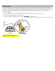
mass of the bar was considered to be 5 Kg and the length of the cord and the bar to be 1m. The
MATLAB code is given below.
% to find the eigen values and the eigen vectors.
l1=1;
l2=1;
m2=5;
g=9.81;
w2=m2*g;
M=[m2*l1^2 (m2*l1*l2)/2;(m2*l1*l2)/2 (m2*l1^2)/3];
K=[l1*w2 0;0 (w2*l2)/2];
[v,d]=eig(K,M)
The columns ‘v’ represent the eigen vectors corresponding to each eigen value ‘d’.
‘M’ represents the inertia matrix and ‘K’ represents the stiffness matrix. The square root of the
eigen values gives the natural frequencies of the system.
The eigen values were found to be 6.2892 and 91.8108 and the corresponding eigen vectors were
⎧0.6661⎫
⎧− 0.4885⎫
⎨ ⎬and
⎨ ⎬respectively.
⎩0.7458⎭
⎩ 0.8726 ⎭
Initial response
To plot the initial response of the system the original nonlinear differential equation has to be
used. Moreover the second order differential equation has to be converted into a vector of first
φ = y(1);
.
φ = y(2);
θ = y(3);
.
θ = y(4);
order differential equation. This step is done by following the procedure given below.
Substituting the above relations in the original nonlinear differential equation, we get the
following nonlinear first order differential equation, which when represented in matrix form is
. ⎧
y(2)
⎫
⎡1
0 0 0 ⎤⎧
⎫
⎪
⎪
− ⎪
⎢
− ⎪
(1)
2
m ⎥
sin( (3) (1))
2l2
cos( y(3)
y(1))
y
m2l2θ
y y
⎪−
sin +
⎪ ⎪
⎪
⎢0
m 0
.
2l
w2
φ
1
2 ⎥ y(2)
2
⎢0
0 1 0 ⎥⎨
. ⎬ = ⎨
y(4)
⎬
⎢
⎢0
⎢⎣
m2l1l
2
cos( y(3)
− y(1))
2
0
m2l
3
2
2
⎥⎪y(3)
⎪
⎥⎪
. ⎪
⎥⎦
⎩y(4)
⎭
⎪
⎪
⎪
⎩
− w l
2 2
sinθ
+ m2l1l
2
. 2
2
φ
sin( θ −φ)
⎪
⎪
⎪
⎭