Chapter 6: Impedance measurements

Acoustic impedance measurements
S u1u2 is the cross-spectrum of both probes and S u1u1 the auto-spectrum of
probe u 1 . Rewriting the transfer function H 2u results in an expression for the
reflection coefficient at the sample material (x=0):
ik ( L−s)
ikL
e − H2u
( ω)
e
−ik ( L−s)
−ikL
−
2u
( ω)
R( ω)
=
e H e
(6.11)
Analogously to the ratio of the velocities measured at x=L and x=L-s, it
is possible to define a quotient of p 1 and p 2 , yielding:
H
S e + R e
ik ( L−s) −ik ( L−s)
( )
p1 p2
2
ω = =
−
p ikL ikL
S
p p
e + R e
1 1
(6.12)
where p 1 and p 2 represent the measured pressures at x=L and x=L-s.
Applying some mathematics, it can be deduced that there is a mutual
and unique relation between H 2u and H 2p , i.e.
H
2iks
iks
(1 + e ) H 2 p − 2e
= (6.13)
iks
2
2e
H − (1 + e )
2u
iks
2 p
Expression (6.13) shows that, since H 2u and H 2p are uniquely related and
only the spacing s (not even L) appears, the 2u and 2p-method are not
fundamentally different.
10 2
10 2
10 1
10 1
|H |
10 0
|H |
10 0
10 -1
10 -1
10 -2
10 -2
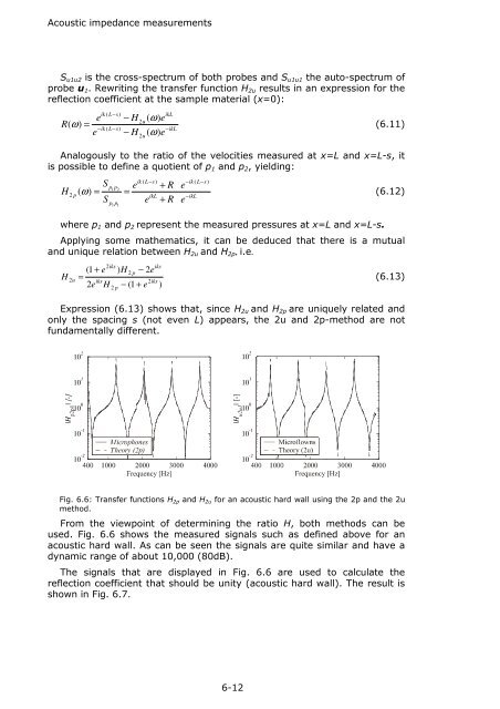
Fig. 6.6: Transfer functions H 2p and H 2u for an acoustic hard wall using the 2p and the 2u
method.
From the viewpoint of determining the ratio H, both methods can be
used. Fig. 6.6 shows the measured signals such as defined above for an
acoustic hard wall. As can be seen the signals are quite similar and have a
dynamic range of about 10,000 (80dB).
The signals that are displayed in Fig. 6.6 are used to calculate the
reflection coefficient that should be unity (acoustic hard wall). The result is
shown in Fig. 6.7.
6-12