editorial team

EDITORIAL TEAM 

Editors 

Celso Augusto Guimarães Santos, Federal University of Paraíba, Brazil 

Masuo Kashiwadani, Ehime University, Japan 

Dragan Savic, University of Exeter, United Kingdom 

Vicente L. Lopes, Texas State University, United States 

Associate Editors 

Koichi Suzuki, Ehime University, Japan 

Hafzullah Aksoy, Istanbul Technical University, Turkey 

António Pais Antunes, University of Coimbra, Portugal 

Roberto Leal Pimentel, Federal University of Paraíba, Brazil 

Max Billib, Hannover University, Germany 

Bernardo Arantes do Nascimento Teixeira, Federal University of São Carlos, Brazil 

Generoso de Angelis Neto, State University of Maringá, Brazil 

FOCUS and SCOPE 

Journal of Urban and Environmental Engineering (JUEE) provides a forum for original papers and for the exchange of 

information and views on significant developments in urban and environmental engineering worldwide. The scope of the 

journal includes: 

(a) Water Resources and Waste Management: This topic includes (i) waste and sanitation; (ii) environmental 

issues; (iii) the hydrological cycle on the Earth; (iv) surface water, groundwater, snow and ice, in all their physical, 

chemical and biological processes, their interrelationships, and their relationships to geographical factors, atmospheric 

processes and climate, and Earth processes including erosion and sedimentation; (v) hydrological extremes and their 

impacts; (vi) measurement, mathematical representation and computational aspects of hydrological processes; (vii) 

hydrological aspects of the use and management of water resources and their change under the influence of human 

activity; (viii) water resources systems, including the planning, engineering, management and economic aspects of 

applied hydrology. 

(b) Constructions and Environment: Buildings and infrastructure constructions (bridges/footbridges, pipelines etc) 

are part of every urban area. In recent years there is a growing interest in seeking rationality of construction systems, in 

balance with environmental adequacy and harmony in an urban area. This involves, among others, adequacy of structural 

systems (shapes, functionality, rational design etc), use of alternative materials for construction (recycled, 

environmentally friendly materials etc) and solutions seeking energy efficiency. 

(c) Urban Design: This topic covers the arrangement, appearance and functionality of towns and cities, and in 

particular the shaping and uses of urban public space (e.g. streets, plazas, parks and public infrastructure), including also 

urban planning, landscape architecture, or architecture issues (e.g. thermic and acoustic comfort). 

(d) Transportation Engineering: This topic covers such area as Traffic & Transport Management, Rail Transport, Air 

Transport, International Transport, Logistics/Physical Distribution/Supply Chain Management, Management Information 

Systems & Computer Applications, Motor Transport, Regulation/Law, Transport Policy, and Water Transport.

SUMMARY 

LEAD DISTRIBUTION BY URBAN SEDIMENTS ON IMPERMEABLE AREAS OF PORTO 

ALEGRE – RS, BRAZIL……………………………………………………………………………………………….. 1-8 

Leidy Luz Garcia Martinez, Cristiano Poleto 

MODELING OF WEATHER DATA FOR THE EAST ANATOLIA REGION OF TURKEY…………….. 9-22 

Ebru Akpinar, Sinan Akpinar 

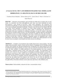
VIABILITY OF PRECIPITATION FREQUENCY USE FOR RESERVOIR SIZING IN 

CONDOMINIUMS………………………………………………………………………………………………………. 23-28 

Isabelle Yruska de Lucena Gomes Braga, Celso Augusto Guimarães Santos 

STUDY ON NEED FOR SUSTAINABLE DEVELOPMENT IN EDUCATIONAL INSTITUTIONS – 

A CASE STUDY OF COLLEGE OF ENGINEERING- GUINDY, CHENNAI……………………………….29-36 

Gobinath Ravindran, R. Nagendran 

DEFLUORIDATION OF DRINKING WATER BY ELECTROCOAGULATION/ 

ELECTROFLOTATION - KINETIC STUDY……………………………………………………………………… 37-45 

Bennajah Mounir, Mostafa Maalmi, Yassine Darmane, Mohammed Ebn Touhami

Martínez and Poleto 

1 

J U E E 

Journal of Urban and Environmental 

Engineering, v.4, n.1, p.1-8 

ISSN 1982-3932 

doi: 10.4090/juee.2010.v4n1.001008 

Journal of Urban and 

Environmental Engineering 

www.journal-uee.org 

LEAD DISTRIBUTION BY URBAN SEDIMENTS ON 

IMPERMEABLE AREAS OF PORTO ALEGRE – RS, BRAZIL 

Leidy L.G. Martínez 1∗ and Cristiano Poleto 2 

1 Hidraulic Research Institute, Federal University of Rio Grande do Sul, Brazil 

2 State University of Maringá, Brazil 

Received 23 April 2009; received in revised form 15 June 2010; accepted 18 June 2010 

Abstract: 

Keywords: 

Heavy metals, like lead (Pb), are subproducts of industrial activities; however, in recent 

years, studies have shown that even in non-industrial areas, elevated concentrations of 

this element have been found. In this study, Pb concentrations were measured in 20 

composite samples of urban sediments collected in an urban watershed of 4.85 km² 

with three types of soil use (commercial/residential, commercial and industrial) in the 

city of Porto Alegre, RS, Brazil. Concentrations were determined by acid digestion 

(EPA 3050) of the 209 µm, 150 µm, 90 µm, 63 µm and 45 µm fractions followed by 

atomic emission spectrophotometry with inductively coupled plasma. Average values 

of 178.1 µg.g -1 (± 332); 226.5 µg.g -1 (± 500); 245.2 µg.g -1 (± 454.1); 272.4 µg.g -1 (± 

497.3) and 251.5 µg.g -1 (± 322.6) were obtained in the 209, 150, 90, 63 and 45 µm 

fractions, respectively. Concentrations of the metals studied were interpolated and 

represented geographically using Idrisi © Andes. Results show that the greatest 

concentrations are located in the commercial part of the study area, characterized as 

presenting high vehicle flow most of the day, with this being considered a potential 

source of lead. All concentrations were above that of the local background. Studies of 

this type are important because they make the establishment of control targets possible 

within sustainable management of water resources, allowing inferences regarding 

future pollution scenarios of local water resources. 

Urban sediment; diffuse pollution; GIS; lead 

© 2010 Journal of Urban and Environmental Engineering (JUEE). All rights reserved. 

∗ Correspondence to: Leidy L.G. Martínez, Tel.: + 55 51 3308 6686. 

E-mail: luxgm@yahoo.es 

Journal of Urban and Environmental Engineering (JUEE), v.4, n.1, p.1-8, 2010


2 

INTRODUCTION 

Most South American cities present accelerated growth 

trends; however, they are disorganized, generating 

negative impacts especially on bodies of water (Poleto 

et al,. 2009a; Deletic et al,. 1997), principally due to the 

increase of impermeable surfaces like roadways, roofs, 

parking lots, among other things, which reduce the rate 

of infiltration and increase surface runoff, thus 

increasing transport of urban sediment and pollutant 

loads to watercourses (Poleto et al., 2009b; Taylor 

2007; Charlesworth et al., 2003; Deletic et al., 1997). 

Urban drainage networks are responsible for conveying 

these loads and it is now known that they constitute 

important sources of degradation of rivers, lakes and 

estuaries Horowitz (2009), (Deletic et al., 1997). 

Sediments in urban areas are submitted to man-made 

alterations from different sources, as for example, the 

input of organic matter coming from discarding sewage 

in a clandestine manner, in the same way as particles of 

human origin present in large quantities in urban 

environments, such as glass particles, metallic particles, 

residues from industrial processes and civil 

construction, which present chemical and mineralogical 

properties different from sediment particles from natural 

sources, which results in these sediments interacting in a 

different way within the environment (Poleto & 

Martínez, 2009); Taylor (2007). Sediments deposited in 

roadways have become, through time, an important 

means for determining the human contribution of 

pollutants, especially that of heavy metals. The 

ubiquitous nature of road deposited sediments, their 

ease of sampling, their strong association with 

automobile emissions, and their relationship with 

nonpoint source pollution make them a valuable archive 

of environmental information (Sutherland 2003). 

More precisely, one of the chemical characteristics 

of vital importance in the study of urban sediments is 

adsorption of heavy metals. Banerjee (2003) defines the 

behavior of heavy metals in terms of the most common 

different solid phases found in urban sediments in Table 1. 

Affinity of heavy metals by sediments is strongly 

influenced by particle size (Deletic et al., 1997; 

Charlesworth et al., 2003; Sutherland, 2003; Taylor, 

2007; Poleto et al., 2009a). There is sufficient evidence 

that shows the fact that sediments are enriched with 

heavy metals, above all in the fine particle fraction. In a 

similar way to sediments in other environments, 

increase in the pollutant load in finer sized particles is 

generally associated with the increase of surface area in 

smaller sized particles, providing greater space for 

adsorption of metals in clay minerals or in organic 

matter present in sediment particles. Understanding that 

heavy metal loads are heterogeneously distributed is 

important in the formulation of pollution management 

and control strategies (Horowitz, 2009; Poleto et al., 

2009b; Taylor, 2007). Fergusson & Ryan (1984) studied 

Table 1. Affinity of heavy metals in sediments 

Solid phase fraction 

Exchangeable 

Carbonate 

Fe-Mn oxide bonding 

Organic matter 

Residual 

Adapted from: Banerjee (2003). 

Affinity of heavy metal 

Cd > Pb > N i> Zn > Cu > Cr 

Cd > Zn > Pb > Ni > Cu > Cr 

Zn > Pb > Ni = Cu > Cd > Cr 

Cu > Pb > Zn > Ni > Cd > Cr 

Cr > Ni > Cu > Cd > Pb > Zn 

the composition of particles deposited in urban areas, 

specifically particle size and the sediment source; they 

found that many of the elements analyzed increased 

with reduction in particle size, a result corroborated by 

Al-Rajhi et al. (1996). 

In urban environments, heavy metals are part of our 

daily activities and many of them enter in the urban 

environment as subproducts of economic activities 

which are considered typical in urbanizing watersheds 

(Poleto & Charlesworth, 2010; Poleto et al., 2009a; 

Poleto & Martínez 2009; Irvine et al., 2009); in the case 

of lead, it frequently appears as a subproduct from 

petroleum and coal combustion; tire, oil, paint and 

welded part residues (Horowitz, 2009; Poleto & Merten, 

2008; Charlesworth & Lees 1999). Lead concentration 

values are variable and depend in large part on 

surrounding local conditions; Sutherland (2003) found 

that 51% (221 µg.g -1 ) of the lead load present in 

sediments deposited in urban roadways in Hawaii were 

found in the < 63 µm fraction; Robertson et al. (2003) 

found concentrations of 354 µg.g -1 within the city of 

Manchester (United Kingdom); Charlesworth et al. 

(2003) found average values of 48 and 47.1 µg.g -1 in the 

cities of Birmigham and Coventry (United Kingdom), 

respectively; Irvine et al. (2009) reported values of 276 

µg.g -1 in the city of Hamilton, Ontario (Canada); an 

average value of 230.52 µg.g -1 with a maximum of 3060 

µg.g -1 were found by Yongming et al. (2006) in the 

province of Xi’an in China; McAlister et al. (2005) 

reported concentrations from 200 to 700 µg.g -1 in areas 

with diverse soil uses in the city of Rio de Janeiro 

(Brazil) and Poleto et al. (2009) found concentrations 

from 16 to 110 µg.g -1 in 20 cities in the South of Brazil. 

Sediments deposited in roadways are commonly 

associated with risks to the environment and to 

human health, mainly in children (Taylor, 2007; 

Charlesworth et al., 2003; Al-Rajhi et al., 1996). 

Environmental and health effects initially depend on 

the mobility and availability of the elements, and the 

mobility and availability in terms of their chemical 

speciation and fractionation within or on particles 

(Banerjee, 2003). In the case of lead, there is 

evidence that indicates that exposure to this metal 

(inhalation or through consumption of contaminated 

foods) can trigger problems in the central nervous 

system, as well as having carcinogenic effects (Wang 

et al., 2005). 



3 

In the present study, the lead concentration present in 

20 composite samples of urban sediments collected at 

different points of the Tamandaré Basin (which drains 

into Guaíba Lake) and which present different soil uses 

was evaluated. Lead (Pb) concentrations were 

determined in different granulometric fractions of the 

sediments for the purpose of establishing a correlation; 

afterwards they were geographically represented 

through the use of a GIS, with values corresponding to 

the < 63 µm fraction, considered by diverse studies as 

that which presents the greatest heavy metal adsorption 

capacity. 

MATERIAL AND METHODS 

Study area 

The study area chosen is located between the center 

downtown area and the northern part of the city of Porto 

Alegre, capital of the state of Rio Grande do Sul, in the 

South of Brazil (Fig. 1). 

In accordance with the Koppen (1936) classification, 

the climate in the region is temperate, subtropical and 

humid. The study area is inserted within the urban 

Almirante Tamandaré sub-basin, which drains into Lake 

Guaíba and is georeferenced between the coordinates 

476 561.77 E; 6 676 956.05 S and 481 482.71 E; 

6 682 109.55 S. Within the study area, three areas 

representative of predominant soil uses in the city were 

chosen: industrial (3.0 km²), commercial (1.02 km²) and 

residential/commercial (0.83 km²), as represented in 

Fig. 2. The limits of the study area represent avenues of 

high vehicular traffic volume. 

Sediment monitoring 

During the month of June, composite samples of 

sediments accumulated from the streets of the study area 

were collected. The samples were the result of the 

Fig. 2 Study area. 

composition of various sub-samples of dry sediment 

collected in an area of approximately 200 m² for each 

point chosen (thus reducing the influence of point 

source pollution, making the samples more 

representative), as represented in Fig. 3 and following 

a methodology similar to that used by Poleto et al. 

(2009), Krčmová et al. (2009), Yetimoglu et al. 

(2008), Banerjee (2003), Charlesworth et al. (2003), 

Charlesworth & Lees (1999) and Deletic et al. (1997). 

Approximately 500 g of dry sediment were 

collected for each point (Poleto et al., 2009; 

Sutherland, 2003). 

Samples were collected using a portable vacuum 

without metallic parts and which facilitated the 

collection of samples without direct manual contact 

and which lead to sampling of finer particle fractions. 

Collected samples were deposited in plastic bags and 

refrigerated for later performance of physical and 

chemical analyses. 

Fig. 1 Geographical location of the study area. 

Fig. 3 Sample collection points. 

Adapted from: Poleto et al. (2009a). 


4 


Lead analyses by granulometric fraction 

Each sample collected was submitted to sieving 

(polyethylene sieves – without metallic parts), using 

screens or openings of 45 µm, 63 µm, 90 µm, 150 µm 

and 209 µm, following the methodology used by 

Banerjee (2003) and Charlesworth et al. (2003) and 

which shows the separation of the most important 

granulometric fractions for urban sediment quality 

studies. 

Granulometric analysis was made by a laser particle 

analyzer Cilas ® 1180 located at the Laboratory of the 

UFRGS Density Currents Study Center – Núcleo de 

Estudos de Correntes de Densidade da UFRGS. This 

piece of equipment allows one to differentiate particles 

from 0.04 to 2500 µm. The methodology used is 

described by Poleto et al. (2009a). 

Samples were submitted to acid digestion (HCl, HF, 

HCLO4, HNO3), in accordance with methodology from 

the U. S. Environmental Protection Agency (EPA 

3050). These analyses were duplicated and two USGS 

reference materials (SGR-1b and SCO-1) for quality 

control were used. Afterwards, total metal 

concentrations were determined by inductively coupled 

plasma optical emission spectrometry (ICP-OES) on a 

Perkin Elmer brand piece of equipment by the UFRGS 

Soil Laboratory. 

All equipment and glass items used in the sample 

collection procedure and sample treatments were 

washed with distilled water, remained soaking in a 14% 

(v/v) nitric acid solution for 24 hours and once more 

rinsed with distilled water. 

Interpretation of results 

Descriptive statistics of the concentration data obtained 

from chemical analyses were calculated and, afterwards, 

linear regression of the concentrations was applied in 

terms of particle size for the purpose of establishing a 

correlation between these two variables, widely 

mentioned in studies of this type. In the event that the 

adjusted model presents poor correlation, the best 

adjustment would be applied with the averages from the 

data of each fraction studied, in accordance with that 

suggested by Al-Rajhi et al. (1996). 

After this process, the non parametric Kruskall- 

Wallis Test was undertaken, followed by the Bonferroni 

test for the purpose of analyzing the significance of the 

sample collection location in respect to the Pb 

concentrations found, in accordance with that suggested 

by Irvine et al. (2009), Norra et al. (2006) and Kuang et 

al. (2004). The statistical analyses were undertaken 

using the software XLSTAT © v. 2009. 

The lead values of the < 63 µm fraction were 

interpolated through the IDW (Inverse Distance Weight) 

method and the result was represented on a thematic 

map using the SIG Idrisi © Andes, which allowed 

visualization of the greatest lead concentration areas 

within the study area, as well as allowing inferences 

regarding the factors which had an influence on these 

results. 

RESULTS AND DISCUSSIONS 

Granulometry of urban sediments 

The results of granulometric analysis undertaken in the 

samples collected in the study area are presented in 

Fig. 4. The < 63 µm fraction, which according to Poleto 

et al. (2009a), Poleto et al. (2009b), Irvine et al. (2009), 

Charlesworth et al. (1999; 2003), Robertson et al. 

(2003) and Sutherland (2003) is strongly correlated with 

the greatest concentrations of heavy metals, represents 

approximately 40% of the sediments collected in the 

area with commercial/residential soil use and 60% for 

the two other sampled areas. Sutherland (2003) found 

that the dominant fraction was the < 63 µm one with 

38% of the total of analyzed fractions. 

Descriptive statistics 

The values of Pb concentrations obtained in the 20 

sediment samples are presented in Table 2. 

The fact of the median being greater than the average 

of the data says that the data distribution is 

asymmetrical to the right, which is corroborated by the 

Fisher coefficient (α = 0.05). This asymmetry obeys the 

peaks of concentration found in some sampling points, 

which generates a considerable standard deviation for 

the data. Yonming et al. (2006) found values from 29 to 

3060 µg.g -1 and a Fisher coefficient of 5.34 in samples 

of urban sediments collected in the Xi’an province in 

Central China, showing the same trend of the values 

found in this study. 

Fig. 4 Granulometric analyses of the urban sediment samples. 



5 

Table 2 Descriptive statistics of lead concentrations (µg.g -1 ) 

Descriptive Statistic 

Particle size (µm) 

209 150 90 63 45 

Minimum 22 39 58 76 86 

Maximum 1500 2300 2100 2300 1300 

Median 91.00 93.00 121.00 123.50 147.00 

Mean 178.10 226.45 245.20 272.35 251.54 

Standard Deviation 331.99 499.99 454.15 497.29 322.59 

Skewness (Fisher) 1.82 2.15 1.81 1.78 1.23 

In the minimum values, one may observe the 

increase in lead concentration with reduction in particle 

size, which is corroborated by Poleto et al. (2009a), 

Irvine et al. (2009), Norra et al. (2006), Kuang et al. 

(2004), Charlesworth et al. (2003), Charlesworth & 

Lees (1999). Maximum values are commonly found in 

this type of study and were cited by Charlesworth et al. 

(2003) who found lead concentrations of 2 582.5 µg.g -1 

for New York and 2241 µg.g -1 for London. Al-Rahji et 

al. (1996) perceived that these maximum values 

increase the standard deviation of the data and usually 

alter the correlations between particle diameter and 

concentrations of heavy metals. 

Lead concentration values were correlated (α = 0.05) 

with the opening of the mesh through a linear model; 

however, the results showed poor correlation, 

established by the value of the regression coefficient 

(R² = 0.005). This is explained by the fact that most of 

the values are outside the statistical confidence interval 

(95%), above all in the 63 to 150 µm fractions. Linear 

regression may be observed in Fig. 5. 

To correct this, the average of the values of the 

concentrations in each one of the fractions was 

calculated and regression models were once more 

calculated. Of all the models tested, the exponential 

model presented the best correlation (R² = 0.87) at the 

same level of significance. This result is similar to that 

reported by Al-Rajhi et al. (1996), who found 

correlations above 80%. Figure 6 presents the result of 

the exponential adjustment of the data obtained. 

Fig. 6 Exponential regression model chosen. 

The mathematical model obtained in this regression 

is presented in Eq. (1). 

Y = 298.4e -0.002x (1) 

where x represents the particle diameter (µm) and Y 

the Pb concentration (µg.g -1 ). 

Results demonstrate that urban sediments are 

enriched with Pb, above all in the fine fraction of the 

particles. In a similar way to sediments in other 

environments, the increase in pollution load in finer 

sized particles is generally associated with the 

increase in surface area in smaller sized particles, 

supplying a greater space for adsorption of metals in 

clay minerals or in the organic matter present in 

sediment particles. Robertson et al. (2003) suggested 

that the particles generated by automotive vehicles 

present a high Fe/Pb ratio and concluded that in their 

case the principal source of lead in urban areas was 

vehicular traffic. 

Understanding that heavy metal loads are 

heterogeneously distributed is important in the 

formulation of pollution management and control 

strategies (Poleto et al., 2009a; Irvine et al., 2009; 

Taylor, 2007; Charlesworth et al., 2003; Sutherland, 

2003). 

Spatial distribution of lead in the study area 

Fig. 5 Lead linear regression in terms of sieve size. 

Studies of lead associated with urban sediment particles 

were the first to be performed for the purpose of 



6 

establishing the risk to human health generated by 

vehicle traffic, which in the past used lead in gasoline in 

abundance (Taylor, 2007; Robertson et al., 2003). The 

results obtained were important in the decision to reduce 

lead concentration in gasoline in many countries. 

To determine what the increase of Pb concentrations 

due to human activity is, there is the need to verify the 

value of the local background. As the study area is 

densely urbanized, it was not possible to find a naturally 

preserved area (without any human interference); for 

that reason we took into consideration the data obtained 

in the studies of Poleto & Merten (2005) and Poleto et 

al. (2008) which were obtained for the same watershed, 

which is a sub-watershed in the Porto Alegre 

metropolitan area. The value found by the authors is 

31.30 µg.g -1 , thus, configuring elevated human 

enrichment in the study area. 

Distribution of concentrations by soil use, 

represented in Fig. 7, shows how the lead concentration 

is greater in the commercial area, even greater than in 

the industrial area where gasoline selling stations and 

industries that use metals as raw material predominate. 

Nevertheless, most of the points sampled in the 

industrial area present a traffic volume in a lower 

proportion than in the two other areas studied. In this 

commercial area, two of the points sampled presented 

values above the average of the rest of the data and 

these points coincide precisely with a street of high city 

bus traffic. At this point, the presence of vehicle oil and 

tire particles on the surface was observed, indicating 

that this potential source would be the main lead 

potential in this area. 

The result of the Kruskall-Wallis Test showed that 

the data is derived from the same population; whereas 

the Bonferroni Test showed that there is no significant 

relationship between the lead concentrations and the 

respective area of sample collection, to a 5% level of 

significance, similar to the results found by 

Charlesworth et al. (2003) in the city of Birmigham. 

The fact that soil use is not correlated with the lead 

concentration may indicate that there is an external 

factor that influences this behavior, which is probably 

the chemical composition of the sediment particles, 

which influences the rate of lead adsorption, in 

accordance with results presented by Banerjee (2003) 

and Robertson et al. (2003) who define that lead is 

associated with the residual fraction > Fe/Mn oxides > 

organic matter > exchangeable fraction > carbonates. 

According to Krčmová, et al. (2009) and Charlesworth 

et al. (2003), it is still difficult to establish the main 

source of lead in urban sediments; nevertheless, some 

studies suggest that the presence of this metal together 

with zinc is associated with tire residues, which 

is directly associated with vehicular traffic volume. 

Fig. 7 Lead distribution by soil use. 

Figure 8 presents the spatial distribution of Pb in the 

study area. 

It is fitting to highlight that the commercial area of 

Porto Alegre presents a high volume of people and that 

high metal concentrations like the lead adsorbed in the 

finer particles may present health risks since this finer 

range is breathable. Likewise, the nearness of these 

areas to Guaíba Lake (main local body of water) may be 

contributing in a significant way to the increase of 

heavy metals in these ecosystems since the Lake is the 

final point in the urban drainage systems of this 

watershed. 

Fig. 8 Spatial distribution of Pb (µg.g -1 ) in urban sediments in the 

study area. 



7 

CONCLUSIONS 

- Pb is a heavy metal which is closely associated with 

urban sediment particles; 

- Samples are composed of large percentages of fine 

particles (< 63 µm) in the three areas monitored; 

- Maximum values of concentration were found in the 

finest particles of the collected sediment samples, 

regardless of the point of origin of the sample; 

- The mathematical model which best explained the 

regression between the Pb concentration and the 

particle size was based on an exponential adjustment 

of the variables; 

- The highest Pb values were found in commercial 

areas, a situation that may be explained in terms of 

vehicular traffic volume and this coincides with other 

studies in different cities in the world; 

- Lead concentrations in urban sediments of the three 

areas went far beyond the local background 

concentration which was adopted; 

- Research should be increased in regard to how to make 

urban systems more sustainable, reducing their 

pollution potential and minimizing the entrance of 

potentially polluting particles into bodies of water that 

pass through these urbanized areas. 

Acknowledgments The Authors would like to thank 

CAPES, CNPq and Soils Analysis Laboratory of 

UFRGS. 

REFERENCES 

Al-Rajhi, M.A., Al-Shayeb , S.M., Seaward, M.R. & Edwards, H.G. 

(1996) Particle size effect for metal pollution analysis of 

atmospherically deposited dust. Atmospheric Environment 30(1), 

145–163. 

Banerjee, A.D.K. (2003) Heavy metal levels and solid phase 

speciation in street dusts of Delhi, India. Environmental Pollution 

23(1), 95–105. doi: 10.1016/S0269-7491(02)00337-8. 

Charlesworth, S.M., Everett, M., McArthy, R., Ordoñez, A. & de 

Miguel, E. (2003) A comparative study of heavy metal 

concentration and distribution in deposited street dusts in a large 

and a small urban area: Birmingham and Coventry, West 

Midlands, UK. Environment International 29(5), 563–573. doi: 

10.1016/S0160-4120(03)00015-1. 

Charlesworth, S.M. & Lees, J.A. (1999) Particulate-associated heavy 

metals in the urban environment: their transport from the source 

to deposit, Coventry, UK. Chemosphere 39(5), 833–848. doi: 

10.1016/S0045-6535(99)00017-X. 

Deletic, A., Maksimovic, C. & Ivetic, M. (1997) Modelling of storm 

wash-off of suspended solids from impervious surfaces. J. Hydr. 

Res. 35(1), 99–118. doi: 10.1080/00221689709498646. 

Fergusson, J.E. & Ryan, D.E. (1984) The elemental composition of 

street dust from large and small urban areas related to city type, 

source and particle size. Sci. Total Envir. 34(1), 101–116. doi: 

10.1016/0048-9697(86)90363-3. 

Horowitz, A.J. (2009) Monitoring suspended sediments and 

associated chemical constituents in urban environments: lessons 

from the city of Atlanta, Georgia, USA Water Quality Monitoring 

Program. J. Soils and Sediments 9(4), 342–363. doi: 

10.1007/s11368-009-0092-y. 

Irvine, K., Perrelli, M.F., Ngoen-klan, R. & Droppo, I. (2009) Metal 

levels in street sediment from an industrial city: spatial trends, 

chemical fractionation, and management implications. J. Soils and 

Sediments 9(4), 328–341. doi: 10.1007/s11368-009-0098-5. 

Krčmová, K., Robertson, D., Cvecková, V. & Rapant, S. (2009) 

Road deposit-sediment, soil and precipitation (RDS) in Bratislava, 

Slovakia: Compositional and spatial assessment of contamination. 

J. Soils and Sediments 9(4), 304–316. doi: 10.1007/s11368-009- 

0097-6. 

Koppen, W. (1936) Das geographisca system der climate. In: 

Handbuch der klimatologie, (Ed. By G. Geiger), 1–44. Gebr, 

Borntraeger. 

Kuang, C., Neumann, T., Norra, S. & Stuben, D. (2004) Land-used 

related chemical composition of street sediments in Beijing. 

Environ. Sci & Poll Res. 11(2), 73–83. doi: 10.1007/BF02979706. 

McAlister, J., Smith, B., Baptista, J. & Simpson, J. (2005) 

Geochemical distribution and bioavailability of heavy metals and 

oxalate in street sediments from Rio de Janeiro, Brazil: a 

preliminary investigation. Environ. Geochem. Health 27(6), 427– 

441. doi: 10.1007/s10653-005-2672-0. 

Norra, S., Lanka-Panditha, M., Kramar, U. & Stuben, D. (2006) 

Mineralogical and geochemical patterns of urban surface soils, the 

example of Pforzheim, Germany. Applied Geochemistry 21(12), 

2064–2081. doi: 10.1016/j.apgeochem.2006.06.014. 

Poleto, C. & Charlesworth, S. (2010) Sedimentology of Aqueous 

Systems. London: Wiley-Blackwell. 

Poleto, C., Bortoluzzi, E. Charlesworth, S. & Merten, G. (2009a) 

Urban sediment particle size and pollutants in Southern Brazil. J. 

Soils and Sediments 9(4), 317 – 327. doi: 10.1007/s11368-009- 

0102-0. 

Poleto, C., Merten, G. & Minella, J.P. (2009b). The identification of 

sediment sources in a small urban watershed in southern Brazil: 

An application of sediment fingerprinting. Environ. Techn. 

30(11), 1145–1153. doi: 10.1080/09593330903112154. 

Poleto, C. & Merten, G.H. (2005) Otimização do uso de metodologia 

de digestão ácida total de sedimentos para a identificação de 

fontes de sedimentos urbanos. In: XVII Simpósio Brasileiro de 

Recursos Hídricos, 16p. 

Poleto, C., Merten, G.H. (2008) Elementos traço em sedimentos 

urbanos e sua avaliação por Guidelines. Holos Environment 8(2), 

100–119. 

Poleto, C. & Martínez, L.G. (2009) Introdução aos Estudos de 

Sedimentos. In: C. Poleto (Ed.), Introdução ao Gerenciamento 

Ambiental. Rio de Janeiro: Editora Interciência. 

Robertson, D.J. & Taylor, K.G., Hoon, S.R. (2003) Geochemical and 

mineral magnetic characterization of urban sediment particulates, 

Manchester, UK. Applied Geochemistry 18(2), 269–282. doi: 

10.1016/S0883-2927(02)00125-7. 

Sutherland, R. (2003) Lead in grain size fractions of roaddeposited 

sediment. Environ. Pollution 121(2), 229–237. doi: 

10.1016/S0269-7491(02)00219-1. 

Taylor, K. (2007) Urban Environments. In: Environmental 

Sedimentology (Ed. by K. Taylor, C. Perry), Manchester: 

Blackwell, 191–222. 

Wang, X., Sato, T., Xing, B. & Tao, S. (2005) Health risks of heavy 

metals to the general public in Tianjin, China via comsumption of 



8 

vegetables and fish. Sci. Total Environ. 350(1), 28–37. doi: 

10.1016/j.scitotenv.2004.09.044. 

Yetimoglu, S. & Ercan, O. (2008) Multivariate analysis of metal 

contamination in street dusts of Istanbul D-100 highway. J. Braz. 

Chem. Soc. 19(7), 1399–1404. 

Yongming, H., Peixuan, D., Junji, C. & Posmentier, E. (2006) 

Multivariate analysis of heavy metal contamination in urban dust 

of Xi’an, Central China. Sci. Total Environ. 355(1), 176–186. doi: 

10.1016/j.scitotenv.2005.02.026. 


Akpinar and Akpinar 

9 

J U E E 



ISSN 1982-3932 

doi: 10.4090/juee.2010.v4n1.009022 




MODELING OF WEATHER DATA FOR THE EAST ANATOLIA 

REGION OF TURKEY 

S. Akpinar¹ and Ebru K. Akpinar² ∗ 

¹Physics Department, Firat University, TR-23119, Elazig, Turkey 

²Department of Mechanical Engineering, Firat University, TR-23119, Elazig, Turkey 

Received 08 March 2010; received in revised form 21 May 2010; accepted 24 May 2010 

Abstract: 

Monthly average daily data of climatic conditions over the period 1994–2003 of cities 

in the east Anatolia region of Turkey is presented. Regression methods are used to fit 

polynomial and trigonometric functions to the monthly averages for nine parameters. 

The parameters namely temperature, maximum–minimum temperature, relative 

humidity, pressure, wind speed, rainfall, solar radiation and sunshine duration are 

useful for renewable energy applications. The functions presented for the parameters 

should enable determination of specific parameter values and prediction of missing 

values. They also provide some insight into the variation of these parameters. The 

models developed can be used in any study related to climatic and its effect on the 

environment and energy. 

Keywords: Energy; environment; temperature, maximum–minimum temperature, relative 

humidity, wind speed, pressure, rainfall, solar radiation, sunshine duration; weather 

parameters 


∗ 

Correspondence to: Dr. Ebru Kavak Akpinar, Mechanical Eng. Department, Firat University, TR-23119, Elazig, 

Turkey. E-mails: ebruakpinar@firat.edu.tr, kavakebru@hotmail.com; Tel: +90-424-2370000/5325; Fax: +90- 

424-2415526. 



10 

INTRODUCTION 

Energy is one of the precious resources in the world. 

Energy conservation becomes a hot topic around 

people, not just for deferring the depletion date of 

fossil fuel but also concerning the environmental 

impact due to energy consumption (Apple et al., 

2006). Performance of environment-related systems, 

such as heating, cooling, ventilating and airconditioning 

of buildings (HVAC systems), solar 

collectors, solar cells, greenhouses, power plants and 

cooling towers, are dependent on weather variables 

like solar radiation, dry-bulb temperature, wet-bulb 

temperature, humidity, wind speed, etc. In order to 

calculate the performance of an existing system or to 

predict the energy consumption of a system in design 

step, the researcher/designer needs appropriate weather 

data (Üner & İleri, 2000). 

Accurate weather data are needed for design 

optimization and performance prediction of solar 

technologies and environmental control systems. 

However, these types of data are not often readily 

available in easily usable form. Analyzed weather data 

developed into an atlas provides useful information on 

renewable energy sources. The modeling of weather 

data results in mathematical and statistical models, 

which enable the determination of data and prediction 

of weather conditions (Dorvlo & Ampratwum, 1999). 

A number of studies are found in the literature 

dealing with the climatic characteristics, solar and 

wind energy related issues for different region of the 

World. Global solar irradiation (GSI) had been 

estimated in a number of studies by the known climatic 

parameters of bright sunshine duration (Sen, 2007; 

Abdul-Aziz et al., 1993), cloud fraction (Norris, 1968; 

Kasten and Czeplak, 1980), air temperature range 

(Bristow & Campbell, 1984), precipitation status 

(McCaskill, 1990), both temperature and rainfall 

(Hansen, 1999) and both sunshine duration and cloud 

(Tasdemiroglu and Sever, 1991; Ododo, 1996), trends 

to years of the weather parameters such as 

temperature, relative humidity, wind speed, dust and 

fog (Al-Garni et al., 1999). 

Climatic differences between urban and suburban 

have been studied by many other authors (Unger, 

1997; Unkasevic, 2001; Roba, 2003; Bernatzky, 1982; 

Wilmers, 1988; Nowak et al., 1998; Yılmaz et al., 

2007). Cañada et al. (1997) developed correlation 

models for global diffuse and tilted irradiation, 

ambient temperature, sunshine hours and specific 

humidity for Valencia in Italy. The coefficients of 

determination of their models were 0.75 or more. 

Coppolino (1994) developed a polynomial relationship 

between the clearness index and relative sunshine 

hours. Raja & Twidell (1994) have carried out 

statistical analysis of measured global insolation data 

for up to 15 years from six locations in Pakistan. They 

obtained cumulative frequency information for 

application when planning solar installations. Dorvlo 

& Ampratwum (1999) developed regression models 

for the weather data of Oman for the period 1987– 

1992. However, there is limited information and 

research dealing with the climatic characteristics, solar 

and wind energy related issues for different region of 

the Turkey in the literature (Tatli et al., 2005; Sahin et 

al., 2006; Sahin 2007; Türkes & Erlat, 2008; Tatli, 

2007). 

This paper models weather data for the 

determination of specific climatic parameter values 

that could be used for developing solar and wind 

technologies and environmental control systems, and 

for the calculation of missing data required for the 

development of a solar and wind atlas for the east 

Anatolia region of Turkey. 


Features of study area 

There are thirteen cities at the east Anatolia region of 

Turkey. Table 1 gives the names and locations of the 

major meteorological stations in the east Anatolia 

region of Turkey. The east Anatolia region of Turkey 

has a typical highland climate, in that it is generally 

cold in winter and hot in summer and there are 

considerable temperature differences between day and 

night. Location of cities at the east Anatolia region of 

Turkey can be shown from Fig. 1. The parameters 

observed daily at the stations are temperature, 

maximum–minimum temperature, relative humidity, 

wind speed, pressure, rainfall, solar radiation and 

sunshine duration. The measurements have been 

carried out by conventional meteorological instruments 

by the Turkish Meteorological State Department 

(TMSD). The Department produces monthly 

summaries of this data. The data for the present study 

is obtained from the summaries of 1994 to 2003. 

Fig. 1 Location of cities in the east Anatolia region of Turkey. 



11 

Table 1. Geographic location of weather stations in the east Anatolia region of Turkey 

Location Longitude east Latitude north 

Agri 43º 03’ 39º 44’ 

Bingöl 40º 29’ 38º 53’ 

Bitlis 42º 06’ 38º 22’ 

Elazig 39º 14’ 38º 41’ 

Erzincan 39º 29’ 39º 44’ 

Erzurum 41º 17’ 39º 55’ 

Hakkari 43º 45’ 37º 34’ 

Igdir 44º 02’ 39º 55’ 

Kars 43º 05’ 40º 36’ 

Malatya 38º 19’ 38º 21’ 

Muş 41º 30’ 38º 44’ 

Tunceli 39º 33’ 39º 07’ 

Van 43º 20’ 38º 28’ 

Modeling of climatic parameters 

Statistical techniques of regression models are 

frequently used to study a set of experimental data. 

Adequacy and validity of the model is performed to 

determine if the model will function in a successful 

manner in its intended operating field. 

Linear regression analysis is a statistical tool by 

which a line is fitted through a set of experimental data 

using the least-squares method. Regression is used in a 

wide variety of applications in order to analyze how a 

single dependent variable is affected by the values of 

one or more independent variables. In this study, 

temperature, maximum temperature, minimum 

temperature, relative humidity, wind speed, pressure, 

rainfall, solar radiation and sunshine duration collected 

for a period of 10 years (1994–2003) is modeled using 

linear regression analysis with 95% confidence level. 

The correlation coefficient (R) was primary criterion 

for selecting the best equation to describe the curve 

equation. In addition to R, the reduced χ 2 as the mean 

square of the deviations between the observed and 

calculated values for the models and root mean square 

error analysis (RMSE) were used to determine the 

goodness of the fit. The higher the values of the R, and 

lowest values of the χ 2 and RMSE, the better the 

goodness of the fit (Akpinar and Akpinar, 2004; 

Akpinar et al., 2006). These can be calculated as: 

R 

n 

n 

2 

∑( Yexp,i 

−Yexpmean 

) −∑( Ypre, 

i −Yexp,i 

) 

i= 

1 

i= 

1 

2 

∑( Yexp,i 

−Yexpmean 

) 

2 

= 

n 

χ 

2 

= 

n 

∑ 

i=1 

i= 

1 

( Yexp 

,i 

− Ypre,i 

) 

N − n 

2 

( Y pre 

− Y ) 

1/ 2 

2 

(1) 

(2) 

N 

⎡ 1 

2 ⎤ 

RMSE = ⎢ ∑ , i exp, i ⎥ 

(3) 

⎣ N i= 

1 

⎦ 

where, Y exp,i is the ith experimentally observed value, 

Y expmean, is the mean of experimentally observed value, 

Y pre,i the ith predicted value, N the number of 

observations and n is the number constants. 

Validation of the established model was made by 

comparing the computed climatic data with the 

observed climatic data in any particular run under 

certain conditions. The performance of the models for 

the climatic data was illustrated. The experimental data 

are generally banded around the straight line 

representing data found by computation, which 

indicates the suitability of the model in describing the 

computed climatic data. 

RESULTS 

The monthly daily summaries over the ten years 1994– 

2003 for the nine meteorological parameters were used 

in developing the models presented (Table 2). The 

summaries are calculated over all the meteorological 

stations where possible. Scatter diagrams of the monthly 

average daily measurements for each year are presented 

in Figs 2, 4, 6, 8, 10, 12, 14, 16, and 18. Polynomial and 

trigonometric models were fitted to the data with the 

months (m: 1–12) as the predictor variable. The 

performance of these models was investigated by 

comparing the determination of coefficient (R), reduced 

chi-square (χ 2 ) and root mean square error (RMSE) 

between the observed and predicted values. Over fitting 

was avoided by listing only the functions with 

statistically non-zero coefficients. 

The monthly average temperatures 

From Fig. 2, it can be seen that there is an evident 

difference at monthly average temperatures between the 

investigated cities. The overall average temperature for 

10 years was found to be about 13.19 o C for Elazig, 

11.50 o C for Erzincan, 5.18 o C for Erzurum, 5.58 o C for 

Kars, 6.83 o C for Agri, 12.74 o C for Igdir, 13.28 o C for 

Tunceli, 10.11 o C for Van, 14.14 o C for Malatya, 12.56 o C 

for Bingöl, 10.69 o C for Muş, 9.87 o C for Bitlis, 10.70 o C 

for Hakkari. While the Erzurum city is the coldest area 


for the whole period, Malatya city is the hottest area for 

the whole period. The monthly average temperatures 

showed changing between -9.4 and 19.4°C for Erzurum 

city, 1.6 and 27.9°C for Malatya city. 

The simple function of the monthly average 

temperature (AT 1 ) fit the ambient temperature data very 

well. The results of statistical analyses undertaken on 

trigonometric model for the monthly average 

temperature are given in Table 3. The model was 

evaluated based on R, χ 2 and RMSE. Generally, R, χ 2 

and RMSE values were varied between 0.99660– 

0.99920, 0.226–0.979 and 0.395–0.823, respectively. 

The function has coefficients of determination of better 

than 0.99 and the lowest values of χ 2 and RMSE for all 

cities. Hence, the trigonometric model (AT 1 ) 

satisfactorily described characteristics of the monthly 

average temperature. Considering trigonometric model 

(AT 1 ), the observed monthly average temperature 

values were compared with calculated ones. Figure 3 

shows the predicted and observed values of monthly 

average temperature. As seen from Fig. 3, there is a 

good agreement between predicted and observed values. 

Table 2. Models for the weather data 

Monthly average 

AT1 = a+b·sin(m)+c·sin((m/2)+d) 

temperature 



maximum temperature 



minimum temperature 


RH = a+b·sin(m)+c·sin((m/2)+d) 

relative humidity 

Monthly average WS = a+b·m+c· (m²)+ 

wind speed 

d·(m 3 )+e·(m 4 ) 

Monthly average P = a+b·m+c· (m²)+ 

pressure 

d·(m 3 )+e·(m 4 ) 

Monthly average RF = a+b·m+c· (m²)+ 

rainfall 

d·(m 3 )+e·(m 4 ) 


SR = a+b·sin(m)+c·sin((m/2)+d) 

solar radiation 

Monthly average SD = a +b·sin(m)+c·sin(2·m)+ 

sunshine duration d·sin(m/2+e) +f·m 


Predicted valu 

30 

25 

20 

15 

10 

5 

0 

-15 -10 -5 

-5 

0 5 10 15 20 25 30 

-10 

-15 

Observed values 

Elazig 

12 

Erzincan 

Erzurum 

Kars 

Agri 

Igdir 

Tunceli 

Van 

Malatya 

Bingöl 

Muş 

Bitlis 

Hakkari 

Fig. 3 Observed and predicted values of the monthly average 

temperatures. 

The monthly average maximum temperatures 

The overall average maximum temperature for 10 years 

was found to be about 19.35 o C for Elazig, 18.05 o C for 

Erzincan, 12.64 o C for Erzurum, 12.72 o C for Kars, 

13.7 o C for Agri, 19.59 o C for Igdir, 19.7 o C for Tunceli, 

15.05 o C for Van, 19.62 o C for Malatya, 18.95 o C for 

Bingöl, 16.52 o C for Muş, 16.22 o C for Bitlis, 15.18 o C for 

Hakkari. While maximum temperatures are at highest 

values in August and July, at lowest values in January. 

While Erzurum is coldest city for the whole period, 

Tunceli is warmest city. Monthly average maximum 

temperatures changed between -3.2 and 28.1°C for 

Erzurum city, 4.8 and 35.3°C for Tunceli city at Fig. 4. 


maximum temperature (AT 2 ) fit the maximum 

temperature data very well. The results of statistical 

analyses undertaken on trigonometric model for the 

monthly average maximum temperature are given in 

Table 4. Generally, R, χ 2 and RMSE values were varied 

between 0.99380–0.99911, 0.194–1.832 and 0.366– 

1.126, respectively. The function has coefficients of 

determination of better than 0.99 and the lowest values 

of χ 2 and RMSE for all cities. Hence, the trigonometric 

model (AT 2 ) satisfactorily described characteristics of 

the monthly average maximum temperature. 

Considering trigonometric model (AT 2 ), the observed 

monthly average maximum temperature values were 

Temperature ( o C) 

30 

25 

20 

15 

10 

5 

0 

-5 

-10 

-15 

1 2 3 4 5 6 7 8 9 10 11 12 

Month 

Elazig 

Erzincan 

Erzurum 

Kars 

Agri 

Igdir 

Tunceli 

Van 

Malatya 

Bingöl 

Muş 

Bitlis 

Hakkari 

Fig. 2 Monthly average temperatures during the years 1994–2003 

for the cities. 

o 

Temperature C ( ) 

40 

35 

30 

25 

20 

15 

10 

5 

0 

-5 

-10 

1 2 3 4 5 6 7 8 9 10 11 12 

Month 

Elazig 

Erzinc an 

Erzurum 

Kars 

Agri 

Igdir 

Tunceli 

Van 

Malatya 

Bingöl 

Muş 

Bitlis 

Hakkari 

Fig. 4 Monthly average maximum temperatures during the years 

1994–2003 for the cities. 



13 

Table 3. The results of statistical analyses according to the model 

(AT 1 ) for the monthly average temperature 

Model 

Monthly average temperature 

= a + b·sin(m) + c·sin((m/2) + d) 

City Constant 

Model 

constants 

R χ 2 RMSE 

a 12.611 

Elazığ b 1.1621 

c -13.494 

0.99 880 0.284 0.443 

d 7.387 

Erzincan 

Erzurum 

Kars 

Agri 

Igdir 

Tunceli 

Van 

Malatya 

Bingöl 

Muş 

Bitlis 

Hakkari 

a 

b 

c 

d 

a 

b 

c 

d 

a 

b 

c 

d 

a 

b 

c 

d 

a 

b 

c 

d 

a 

b 

c 

d 

a 

b 

c 

d 

a 

b 

c 

d 

a 

b 

c 

d 

a 

b 

c 

d 

a 

b 

c 

d 

a 

b 

c 

d 

11.055 

0.7980 

-13.090 

1.1222 

4.5316 

0.1522 

-14.733 

1.0937 

4.9791 

-0.1157 

-13.62 

1.0898 

6.1518 

-0.0053 

-15.555 

1.0638 

12.1077 

0.7469 

-14.032 

1.1860 

12.6769 

1.08504 

-13.893 

1.1011 

9.5648 

0.9691 

-12.663 

1.0589 

13.577 

1.0822 

-13.473 

1.1070 

11.947 

0.8917 

-14.214 

1.088 

9.9987 

0.3676 

-15.886 

1.0665 

9.3095 

0.9693 

-12.917 

1.0696 

10.0726 

0.9066 

-14.744 

1.0315 

0.99 812 0.415 0.536 

0.99 679 0.897 0.788 

0.99 660 0.812 0.750 

0.99 686 0.979 0.823 

0.99 667 0.843 0.764 

0.99 864 0.340 0.485 

0.99 858 0.295 0.452 

0.99 890 0.257 0.422 

0.99 881 0.311 0.464 

0.99 747 0.823 0.755 

0.99 863 0.297 0.454 

0.99 920 0.226 0.395 

compared with calculated ones. Figure 5 shows the 

predicted and observed values of the monthly average 

maximum temperature. There is a good agreement 

between predicted and observed values. 

The monthly average minimum temperatures 

The overall average minimum temperature for 10 years 

was determined to be about 7.06 o C for Elazig, 5.70 o C 

Predicted valu 

40 

35 

30 

25 

20 

15 

10 

5 

0 

-10 -5 -5 0 5 10 15 20 25 30 35 40 

-10 



maximum temperatures. 

Elazig 

Erzincan 

Erzurum 

Kars 

Agri 

Igdir 

Tunceli 

Van 

Malatya 

Bingöl 

Muş 

Bitlis 

Hakkari 


(AT 2 ) for the monthly average maximum temperature 

Model 

Monthly average maximum temperature 

= a + b·sin(m) + c·sin((m/2) + d) 

City Constant 

Model 

constants 

R χ² RMSE 

a 18.688 


c -15.392 

0.99 873 0.390 0.519 

d 1.0942 

Erzincan 

Erzurum 

Kars 

Agri 

Igdir 

Tunceli 

Van 

Malatya 

Bingöl 

Muş 

Bitlis 

Hakkari 

a 

b 

c 

d 

a 

b 

c 

d 

a 

b 

c 

d 

a 

b 

c 

d 

a 

b 

c 

d 

a 

b 

c 

d 

a 

b 

c 

d 

a 

b 

c 

d 

a 

b 

c 

d 

a 

b 

c 

d 

a 

b 

c 

d 

a 

b 

c 

d 

17.409 

0.9192 

-14.693 

7.372 

11.946 

0.4447 

-16.044 

1.0534 

12.082 

0.3482 

-14.860 

1.0479 

12.951 

0.4140 

-17.455 

1.0296 

18.916 

0.6014 

-15.117 

1.1388 

19.021 

1.1777 

-15.723 

1.0700 

14.512 

1.0207 

-12.956 

1.0194 

18.970 

1.0786 

-14.898 

1.114 

18.249 

1.2421 

-16.236 

1.0714 

15.739 

0.5124 

-18.122 

1.0546 

15.580 

1.299 

-15.252 

7.312 

14.509 

1.0466 

-15.983 

1.0133 

0.99 752 0.692 0.692 

0.99 618 1.272 0.938 

0.99 576 1.212 0.916 

0.99 698 1.189 0.907 

0.99 380 1.832 1.126 

0.99 805 0.625 0.658 

0.99 911 0.194 0.366 

0.99 814 0.534 0.608 

0.99 884 0.396 0.523 

0.99 753 1.048 0.852 

0.99 906 0.284 0.443 

0.99 874 0.419 0.538 



(AT 3 ) for the monthly average minimum temperature 

Monthly average minimum temperature 

Model 

= a + b·sin(m) + c·sin((m/2) + d) 

Constant 

constants 

Model 

City 

R χ² RMSE 

a 6.6105 


0.99 587 0.612 0.651 

c -10.65 

d 1.0598 

Erzincan 

Erzurum 

Kars 

Agri 

Igdir 

Tunceli 

Van 

Malatya 

Bingöl 

Muş 

Bitlis 

Hakkari 

a 

b 

c 

d 

a 

b 

c 

d 

a 

b 

c 

d 

a 

b 

c 

d 

a 

b 

c 

d 

a 

b 

c 

d 

a 

b 

c 

d 

a 

b 

c 

d 

a 

b 

c 

d 

a 

b 

c 

d 

a 

b 

c 

d 

a 

b 

c 

d 

5.2303 

0.4802 

-10.804 

1.1158 

-2.9692 

-0.54468 

-12.450 

1.1088 

-1.4663 

-0.4760 

-12.415 

1.1056 

-0.2878 

-0.6481 

-13.192 

1.0772 

6.0989 

0.7160 

-12.440 

1.1732 

6.7410 

0.8648 

-11.326 

1.0893 

4.8203 

0.7447 

-10.920 

1.0275 

8.1937 

0.9545 

-11.172 

1.0725 

6.6144 

0.6555 

-11.942 

1.0754 

4.4451 

-0.06851 

-13.0715 

1.0561 

4.3441 

0.6756 

-10.589 

1.0588 

4.944 

0.6985 

-13.086 

1.0560 

0.99 727 0.461 0.554 

0.99 206 1.593 1.050 

0.99 437 1.119 0.880 

0.99 326 1.519 1.025 

0.99 720 0.558 0.622 

0.99 630 0.616 0.653 

0.99 781 0.340 0.485 

0.99 804 0.318 0.469 

0.99 725 0.508 0.593 

0.99 544 1.006 0.834 

0.99 688 0.454 0.561 

0.99 906 0.208 0.379 

for Erzincan, -2.40 o C for Erzurum, -0.90 o C for Kars, 

0.3 o C for Agri, 6.65 o C for Igdir, 7.23 o C for Tunceli, 

5.28 o C for Van, 8.67 o C for Malatya, 7.13 o C for Bingöl, 

5.01 o C for Muş, 4.8 o C for Bitlis, 5.50 o C for Hakkari 

(Fig. 6). While minimum temperatures are at highest 

values in July, at lowest values in January and February. 

Minimum temperatures reach the warmest values in the 

Malatya. The monthly average minimum temperatures 

demonstrated changing between -1.5 and 20.3°C for 

Malatya city. 



minimum temperature (AT 3 ) fit the minimum 

temperature data very well. The results of statistical 

analyses undertaken on trigonometric model for the 

monthly average minimum temperature are given in 


between 0.99 206–0.99 906, 0.208–1.593 and 0.379– 




model (AT 3 ) satisfactorily described characteristics of 

the monthly average minimum temperature. 

Considering trigonometric model (AT 3 ), the observed 

mean minimum monthly temperature values were 



minimum temperature. There is a good agreement 


o 

Temperature C ( ) 

P redicted valu 

Relative humidity (% 

25 

20 

15 

10 

5 

0 

-5 

-10 

-15 

-20 

1 2 3 4 5 6 7 8 9 10 11 12 

Month 

14 

Elazig 

Erzinc an 

Erzu ru m 

Kars 

Agri 

Ig dir 

Tunceli 

Van 

Malatya 

Bingöl 

Muş 

Bitlis 

Hakkari 

Fig. 6 Monthly average minimum temperatures during the years 


25 

20 

15 

10 

5 

0 

-20 -15 -10 -5 

-5 

0 5 10 15 20 25 

-10 

-15 

-20 


Elazig 

Erzincan 

Erzurum 

Kars 

Agri 

Igdir 

Tunceli 

Van 

Malatya 

Bingöl 

Muş 

Bitlis 

Hakkari 


minimum temperatures. 

90 

80 

70 

60 

50 

40 

30 

20 

10 

0 

1 2 3 4 5 6 7 8 9 10 11 12 

Month 

Elazig 

Erzincan 

Erzurum 

Kars 

Agri 

Igdir 

Tunceli 

Van 

Malatya 

Bingöl 

Muş 

Bitlis 

Hakkari 

Fig. 8 Monthly average relative humidity values during the years 




15 


(RH) for the monthly average relative humidity 

Monthly average relative humidity 

Model 

= a + b·sin(m) + c·sin((m/2) + d) 

Constant 

constants 

Model 

City 

R χ 2 RMSE 

a 58.040 

Elazığ b -4.347 

0.99 772 1.099 0.872 

c 18.755 

d 32.524 

Predicted values 

Erzincan 

Erzurum 

Kars 

Agri 

Igdir 

Tunceli 

Van 

Malatya 

Bingöl 

Muş 

Bitlis 

Hakkari 

90 

80 

70 

60 

50 

40 

30 

a 

b 

c 

d 

a 

b 

c 

d 

a 

b 

c 

d 

a 

b 

c 

d 

a 

b 

c 

d 

a 

b 

c 

d 

a 

b 

c 

d 

a 

b 

c 

d 

a 

b 

c 

d 

a 

b 

c 

d 

a 

b 

c 

d 

a 

b 

c 

d 

63.721 

-1.975 

-12.168 

17.077 

64.193 

-2.596 

14.599 

51.322 

72.1167 

-0.5718 

8.7419 

88.968 

70.881 

-1.754 

11.593 

95.207 

50.135 

-2.866 

12.430 

-17.219 

57.918 

-4.836 

17.532 

20.038 

58.635 

-3.148 

11.330 

45.070 

53.114 

-4.430 

19.897 

7.473 

56.892 

-4.236 

17.329 

32.515 

64.806 

-4.973 

19.633 

70.174 

69.792 

-1.024 

12.222 

95.400 

54.555 

-3.332 

18.185 

0.9574 

0.99 382 1.211 0.915 

0.98 907 3.167 1.481 

0.95 044 5.308 1.917 

0.99 479 0.941 0.807 

0.97 286 5.918 2.024 

0.99 545 1.961 1.165 

0.98 484 2.795 1.391 

0.99 415 3.163 1.480 

0.99 622 1.572 1.043 

0.99 549 2.427 1.296 

0.98 791 2.373 1.282 

0.99 294 3.185 1.485 

20 

20 30 40 50 60 70 80 90 


Elazig 

Erzincan 

Erzurum 

Kars 

Agri 

Igdir 

Tunceli 

Van 

Malatya 

Bingöl 

Muş 

Bitlis 

Hakkari 

Fig. 9 Observed and predicted values of the monthly average relative 

humidity. 

Wind speed (m/s) 

4 

3.5 

3 

2.5 

2 

1.5 

1 

0.5 

0 

1 2 3 4 5 6 7 8 9 10 11 12 

Month 

Elazig 

Erzincan 

Erzurum 

Kars 

Agri 

Igdir 

Tunceli 

Van 

Malatya 

Bingöl 

Muş 

Bitlis 

Hakkari 

Fig. 10 Monthly average wind speed values during the years 1994– 

2003 for the cities. 

The monthly average relative humidity 

Kars city is the most humid area almost throughout the 

period while Igdir is the least humid area. The monthly 

average relative humidity showed changing between 63 

and 81% for Kars city and 38 and 65% for Igdir city 

(Fig. 8). The overall average humidity ratio was about 

a57.69% for Elazig, 63.52% for Erzincan, 63.58% for 

Erzurum, 71.75% for Kars, 70.41% for Agri, 49.58% 

for Igdir, 57.40% for Tunceli, 58.16% for Van, 52.76% 

for Malatya, 56.59% for Bingol, 64% for Muş, 69.25% 

for Bitlis, 53.83% for Hakkari. While relative humidity 

is at highest values in December and January, at lowest 

values in July and August. 

The simple function of the monthly average relative 

humidity (RH) fit the relative humidity data very well. 

The results of statistical analyses undertaken on 

trigonometric model for the monthly average relative 

humidity are given in Table 6. Generally, R, χ 2 and 

RMSE values were varied between 0.95 044–0.99 772, 

1.099–5.308 and 0.872–1.91, respectively. The function 

has coefficients of determination of better than 0.95 and 

the lowest values of χ 2 and RMSE for all cities. 

Therefore, the trigonometric model (RH) satisfactorily 

described characteristics of the monthly average relative 

humidity. Considering trigonometric model (RH), the 

observed monthly average relative humidity values were 



relative humidity. There is a good agreement between 

predicted and observed values. 


4 

3.5 

3 

2.5 

2 

1.5 

1 

0.5 

0 

0 0.5 1 1.5 2 2.5 3 3.5 4 

Elazig 

Erzincan 

Erzurum 

Kars 

Agri 

Igdir 

Tunceli 

Van 

Malatya 

Bingöl 

Muş 

Bitlis 

Hakkari 


Fig. 11 Observed and predicted values of the monthly average wind 

speed. 



16 

Pressure (mbar) 

940 

920 

900 

880 

860 

840 

820 

800 

780 

760 

1 2 3 4 5 6 7 8 9 10 11 12 

Elazig 

Erzincan 

Erzurum 

Kars 

Agri 

Igdir 

Tunceli 

Van 

Malatya 

Bingöl 

Muş 

Bitlis 

Hakkari 

Months 

Fig. 12 Monthly average pressure values during the years 1994– 

2003 for the cities. 

The monthly average wind speed 

The overall average of wind speed for the same period 

was obtained to be approximately 2.69 m/s for Elazig, 

1.47 m/s for Erzincan, 2.80 m/s for Erzurum, 2.54 m/s 

for Kars, 1.50 m/s for Agri, 1.11 m/s for Igdir, 1.21 m/s 

for Tunceli, 2.55 m/s for Van, 1.79 m/s for Malatya, 1.3 

m/s for Bingol, 1.15 m/s for Mus, 1.94 m/s for Bitlis, 

1.60 m/s for Hakkari. The windiest city is Erzurum. The 

monthly average wind speed showed changing between 

2.3 and 3.5 m/s for Erzurum city. 

The simple function of the monthly average wind 

speed (WS) fit the wind speed data very well. The 

results of statistical analyses undertaken on polynomial 

model for the monthly average wind speed are given in 


between 0.82965–0.98047, 0.007–0.049 and 0.067– 



of χ 2 and RMSE for all cities. Therefore, the polynomial 

model (WS) satisfactorily described characteristics of 

the monthly average wind speed. Considering 

polynomial model (WS), the observed monthly average 

wind speed values were compared with calculated ones. 

Figure 11 shows the predicted and observed values of 

the monthly average wind speed. There is a good 

agreement between predicted and observed values. 

The monthly average pressure 

The overall pressure was found to be about 902.74 mbar 

for Elazig, 878.03 mbar for Erzincan, 822.89 mbar for 

Erzurum, 820.79 mbar for Kars, 834.63 mbar for Agri, 

916.84 mbar for Igdir, 903.79 mbar for Tunceli, 831.53 

mbar for Van, 907.19 mbar for Malatya, 886.50 mbar 

for Bingol, 868.95 mbar for Mus, 841.53 mbar for 

Bitlis, 827.20 mbar for Hakkari. While pressure values 

are at highest values in November and December, at 

lowest values in July. Pressure reaches the highest 

values in the Igdir. Pressure values are at lowest values 

in Kars. The monthly average pressure changed between 

818 and 823.8 mbar for Kars city and 832.1 and 838.2 

mbar for Agri city. 


(WS) for the monthly average wind speed. 

Model 

Monthly average wind speed 

= a+b·m+c(m 2 )+d(m 3 )+e(m 4 ) 

City Constant 

Model 

constants 

R χ 2 RMSE 

a 2.023 

Elazığ 

b 0.737 

c -0.188 0.84 615 0.015 0.097 

d 

e 

0.0178 

-0.00 057 

Erzincan 

Erzurum 

Kars 

Agri 

Igdir 

Tunceli 

Van 

Malatya 

Bingöl 

Muş 

Bitlis 

Hakkari 

a 

b 

c 

d 

e 

a 

b 

c 

d 

e 

a 

b 

c 

d 

e 

a 

b 

c 

d 

e 

a 

b 

c 

d 

e 

a 

b 

c 

d 

e 

a 

b 

c 

d 

e 

a 

b 

c 

d 

e 

a 

b 

c 

d 

e 

a 

b 

c 

d 

e 

a 

b 

c 

d 

e 

a 

b 

c 

d 

e 

1.086 

0.0634 

0.0790 

-0.0155 

0.00 071 

2.031 

0.131 

0.0969 

-0.018 

0.00 084 

1.517 

0.391 

0.0244 

-0.0111 

0.00 055 

0.819 

0.0071 

0.1132 

-0.0185 

0.000 772 

0.655 

0.005 955 

0.101 663 

-0.01 795 

0.000 794 

0.939 

0.2319 

-0.0277 

-0.00 146 

0.000 189 

1.970 

0.3716 

-0.0725 

0.00 665 

-0.00 025 

0.953 

0.5166 

-0.063 

0.00 166 

0.000 018 

0.9186 

-0.112 

0.112 

-0.0158 

0.000 605 

0.6712 

-0.0738 

0.1176 

-0.0175 

0.000 692 

2.022 

0.0392 

-0.0117 

0.0012 

-0.00 006 

0.392 929 

0.523 326 

-0.05 629 

0.002 995 

-0.00 013 

0.92 905 0.017 0.103 

0.90 236 0.049 0.174 

0.96 062 0.021 0.113 

0.92 233 0.027 0.130 

0.94 967 0.012 0.088 

0.82 965 0.018 0.104 

0.88 004 0.010 0.078 

0.94 573 0.016 0.100 

0.96 260 0.009 0.073 

0.97 545 0.007 0.067 

0.87 855 0.009 0.074 

0.98 047 0.009 0.072 



17 

The simple function of the monthly average (P) fit 

the pressure data very well. The results of statistical 

analyses undertaken on polynomial model for the 

monthly average pressure are given in Table 7. 

Generally, R, χ 2 and RMSE values were varied between 

0.83 395–0.96 460, 0.728–2.286 and 0.669–1.186, 

respectively. The function has coefficients of 


of χ 2 and RMSE for all cities. The polynomial model 

(P) satisfactorily described characteristics of the 

monthly average pressure. Considering polynomial 

model (P), the observed monthly average pressure 

values were compared with calculated ones (Fig. 13). 

As seen from Fig. 13, there is a good agreement 


The mean rainfall 

The overall average pressure is found to be about 

32.65 mm for Elazig, 32.15 mm for Erzincan, 32.53 mm 

for Erzurum, 41.26 mm for Kars, 41.32 mm for Agri, 

20.78 mm for Igdir, 71.61 mm for Tunceli, 31.32 mm 

for Van, 29.94 mm for Malatya, 79.89 mm for Bingol, 

65.03 mm for Mus, 93.49 mm for Bitlis, 61.61 mm for 

Hakkari. While rainfall values are at highest values in 

April and May, at lowest values in August. Rainfall 

reaches the highest values in the Bitlis. Rainfall values 

are at lowest values in Igdir. The monthly average 

rainfall showed changing between 3.6 and 196.4 mm for 

Bitlis city and 6.5 and 46.1 mm for Igdir city. 


Rainfall (mm 

940 

920 

900 

880 

860 

840 

820 

800 

800 820 840 860 880 900 920 940 

Elazig 

Erzincan 

Erzurum 

Kars 

Agri 

Igdir 

Tunceli 

Van 

Malatya 

Bingöl 

Muş 

Bitlis 

Hakkari 

Observed Values 


pressure. 

200 

180 

160 

140 

120 

100 

80 

60 

40 

20 

0 

1 2 3 4 5 6 7 8 9 10 11 12 

Elazig 

Erzincan 

Erzurum 

Kars 

Agri 

Igdir 

Tunceli 

Van 

Malatya 

Bingöl 

Muş 

Bitlis 

Hakkari 

Month 

Fig. 14 Monthly average rainfall values during the years 1994–2003 

for the cities. 


200 

180 

160 

140 

120 

100 

80 

60 

40 

20 

0 

0 20 40 60 80 100 120 140 160 180 200 

Elazig 

Erzincan 

Erzurum 

Kars 

Agri 

Igdir 

Tunceli 

Van 

Malatya 

Bingöl 

Muş 

Bitlis 

Hakkari 



rainfall. 

The simple function of the monthly average rainfall 

(RF) fit the rainfall data very well. The results of 

statistical analyses undertaken on polynomial model for 

the monthly average rainfall are given in Table 9. 

Generally, R, χ 2 and RMSE values were varied between 

0.70 915–0.98 088, 115.818–2075.940 and 8.220– 



of χ 2 and RMSE for all cities. Hence, the polynomial 

model (RF) satisfactorily described characteristics of the 

monthly average rainfall. Considering polynomial 

model (RF), the observed the monthly average rainfall 

values were compared with calculated ones (Fig. 15). 

There is a good agreement between predicted and 

observed values. 

The monthly average direct solar radiation 

The overall average of solar radiation for the same 

period is obtained to be approximately 363.06 cal/cm 2 

for Elazig, 356.69 cal/cm 2 for Erzincan, 369.72 cal/cm 2 

for Erzurum, 338.37 cal/cm 2 for Kars, 314.26 cal/cm 2 

for Agri, 344.58 cal/cm 2 for Igdir, 387.25 cal/cm 2 for 

Tunceli, 449.39 cal/cm 2 for Van, 382.37 cal/cm 2 for 

Malatya, 373.01 cal/cm 2 for Bingol, 339.51 cal/cm 2 for 

Mus, 340.99 cal/cm 2 for Bitlis, 378.92 cal/cm 2 for 

Hakkari. While direct solar radiation values are at 

highest values in June and July, at lowest values in 

December. Direct solar radiation reaches the highest 

values in the Tunceli. 

Direct solar radiation (cal/cm 2 ) 

800 

700 

600 

500 

400 

300 

200 

100 

0 

1 2 3 4 5 6 7 8 9 10 11 12 

Elazig 

Erzincan 

Erzurum 

Kars 

Agri 

Igdir 

Tunceli 

Van 

Malatya 

Bingöl 

Muş 

Ardahan 

Bitlis 

Hakkari 

Month 

Fig. 16 Monthly average solar radiation values during the years 




18 


(P) for the monthly average pressure 

Model 

Monthly average pressure 

= a+b·m+c(m 2 )+d(m 3 )+e(m 4 ) 

City 

Constant 

constants 

Model 

R χ 2 RMSE 

a 902.284 

Elazığ 

b 5.0578 

c -2.327 0.94 263 1.868 1.072 

d 

e 

0.2966 

-0.0112 

Erzincan 

Erzurum 

Kars 

Agri 

Igdir 

Tunceli 

Van 

Malatya 

Bingöl 

Muş 

Bitlis 

Hakkari 

a 

b 

c 

d 

e 

a 

b 

c 

d 

e 

a 

b 

c 

d 

e 

a 

b 

c 

d 

e 

a 

b 

c 

d 

e 

a 

b 

c 

d 

e 

a 

b 

c 

d 

e 

a 

b 

c 

d 

e 

a 

b 

c 

d 

e 

a 

b 

c 

d 

e 

a 

b 

c 

d 

e 

a 

b 

c 

d 

e 

880.768 

0.2636 

-0.7429 

0.1207 

-0.00501 

822.793 

-0.1523 

-0.2463 

0.05768 

-0.00292 

821.693 

-1.808 

0.3053 

-0.0054 

-0.00058 

833.869 

0.7709 

-0.6021 

0.10181 

-0.00459 

920.707 

1.5712 

-1.4437 

0.2048 

-0.00785 

903.710 

4.1956 

-1.9108 

0.2376 

-0.0087 

829.202 

2.9758 

-1.2465 

0.1686 

-0.00691 

907.553 

4.0417 

-1.9701 

0.2521 

-0.00944 

885.310 

4.8864 

-2.1285 

0.2677 

-0.01008 

867.718 

4.8704 

-2.1587 

0.2768 

-0.01065 

839.499 

2.8874 

-1.2416 

0.16710 

-0.00676 

825.666 

5.2156 

-2.1874 

0.27324 

-0.01035 

0.90 961 1.518 0.966 

0.87 859 0.931 0.757 

0.91 362 0.728 0.669 

0.88 911 1.324 0.902 

0.96 460 1.399 0.928 

0.93 011 1.831 1.061 

0.83 395 1.567 0.982 

0.93 946 1.801 1.053 

0.91 095 2.286 1.186 

0.92 736 1.680 1.017 

0.86 872 1.346 0.910 

0.92 909 1.352 0.912 


(RF) for the monthly average rainfall 

Model 

Monthly average rainfall 

= a+b·m+c(m 2 )+d(m 3 )+e(m 4 ) 

City Constant 

Model 

constants 

R χ 2 RMSE 

a -56.982 

Elazığ 

b 107.576 

c -31.259 0.86 088 199.420 10.786 

d 

e 

3.221 

-0.1086 

Erzincan 

Erzurum 

Kars 

Agri 

Igdir 

Tunceli 

Van 

Malatya 

Bingöl 

Muş 

Bitlis 

Hakkari 

a 

b 

c 

d 

e 

a 

b 

c 

d 

e 

a 

b 

c 

d 

e 

a 

b 

c 

d 

e 

a 

b 

c 

d 

e 

a 

b 

c 

d 

e 

a 

b 

c 

d 

e 

a 

b 

c 

d 

e 

a 

b 

c 

d 

e 

a 

b 

c 

d 

e 

a 

b 

c 

d 

e 

a 

b 

c 

d 

e 

-52.909 

87.434 

-24.342 

2.5168 

-0.0871 

-51.482 

71.919 

-17.286 

1.604 

-0.0514 

7.777 

1.091 

6.258 

-1.110 

0.0494 

-61.609 

100.500 

-25.801 

2.451 

-0.0782 

-28.595 

40.091 

-8.296 

0.6222 

-0.01527 

-32.314 

163.579 

-51.424 

5.375 

-0177 

-51.714 

89.996 

-25.495 

2.5873 

-00855 

-29.828 

80.942 

-24.104 

2.479 

-0.0825 

-29.922 

183.345 

-56.892 

5.789 

-0.184 

-49.587 

172.713 

-53.263 

5.546 

-0.1847 

-120.213 

291.074 

-86.801 

8.895 

-0.293 

-10.777 

131.047 

-39.702 

3.869 

-0.116 

0.70 915 2075.940 34.799 

0.72 121 205.650 10.953 

0.88 245 125.651 8.561 

0.71 498 388.614 15.056 

0.74 827 117.670 8.285 

0.95 607 306.989 13.382 

0.87 435 128.233 8.649 

0.89 658 115.818 8.220 

0.98 088 195.252. 10.672. 

0.97 455 153.141 9.452 

0.96 716 460.725 16.394 

0.95 756 292.439 13.061 



19 


(SR) for the monthly average solar radiation 

Model 

Monthly average solar radiation = 

a+b·sin(m)+c·sin((m/2)+d) 

City Constant 

Model 

constants 

R χ 2 RMSE 

a 352.441 


c 227.146 

0.99 783 142.643 9.937 

d -158.72 

Erzincan 

Erzurum 

Kars 

Agri 

Igdir 

Tunceli 

Van 

Malatya 

Bingöl 

Muş 

Bitlis 

Hakkari 

a 

b 

c 

d 

a 

b 

c 

d 

a 

b 

c 

d 

a 

b 

c 

d 

a 

b 

c 

d 

a 

b 

c 

d 

a 

b 

c 

d 

a 

b 

c 

d 

a 

b 

c 

d 

a 

b 

c 

d 

a 

b 

c 

d 

a 

b 

c 

d 

347.345 

10.931 

202.003 

142.948 

361.205 

26.720 

-186.07 

45.543 

330.177 

18.630 

178.119 

180.663 

305.321 

21.509 

193.157 

-20.477 

334.978 

11.145 

205.287 

-114.693 

376.126 

23.556 

239.240 

61.156 

438.504 

20.299 

-234.433 

-11.019 

371.562 

18.861 

231.646 

36.048 

361.769 

24.394 

242.097 

-246.684 

329.416 

17.294 

-216.399 

-42.496 

330.900 

26.0458 

-218.294 

-42.469 

370.263 

15.914 

-186.987 

51.843 

0.99 862 71.532 7.037 

0.99 617 173.440 10.958 

0.99 678 132.002 9.560 

0.99 689 149.901 10.187 

0.99 767 125.225 9.311 

0.99 719 207.375 11.982 

0.99 823 124.832 9.296 

0.99 893 73.750 7.145 

0.99 705 222.535 12.412 

0.99 836 98.421 8.255 

0.99 537 286.837 14.092 

0.99 658 153.909 10.322 

Direct solar radiation values are at lowest values 

in Agri. The monthly average direct solar radiation 

demonstrated changing between 139.78 and 

628.3 cal/cm² for Tunceli city, 102.01 and 504.6 

cal/cm 2 for Agri city. 

The simple function of the monthly average solar 

radiation (SR) fit the solar radiation data very well. The 

results of statistical analyses undertaken on 

trigonometric model for the monthly average solar 


800 

700 

600 

500 

400 

300 

200 

100 

0 

0 100 200 300 400 500 600 700 800 

Elazig 

Erzincan 

Erzurum 

Kars 

Agri 

Igdir 

Tunceli 

Van 

Malatya 

Bingöl 

Muş 

Bitlis 

Hakkari 


Fig. 17 Observed and predicted values of the monthly average solar 

radiation. 

Sunshine duration (min) 

800 

700 

600 

500 

400 

300 

200 

100 

0 

1 2 3 4 5 6 7 8 9 10 11 12 

Elazig 

Erzincan 

Erzurum 

Kars 

Agri 

Igdir 

Tunceli 

Van 

Malatya 

Bingöl 

Muş 

Ardahan 

Bitlis 

Hakkari 

Month 

Fig. 18 Monthly average sunshine duration values during the years 


radiation are given in Table 10. Generally, R, χ 2 and 

RMSE values were varied between 0.99 537–0.99 893, 

71.532–286.837 and 7.037–14.092, respectively. The 

function has coefficients of determination of better than 

0.99 and the lowest values of χ 2 and RMSE for all cities. 

Hence, the trigonometric model (SR) satisfactorily 

described characteristics of the monthly average solar 

radiation. Considering trigonometric model (SR), the 

observed monthly average solar radiation values were 

compared with calculated ones (Fig. 17). As seen from 

Fig. 17, there is a good agreement between predicted and 

observed values. 

The mean sunshine duration 

The overall average sunshine duration for 10 years is 

found to be about 464.76 min for Elazig, 369.48 min for 

Erzincan, 381.33 min for Erzurum, 396.75 min for Kars, 

389.83 min for Agri, 393.25 min for Igdir, 441.33 min 

for Tunceli, 506.08 min for Van, 476 min for Malatya, 

391.33 min for Bingol, 439.58 min for Mus, 347.58 min 

for Bitlis, 468.66 min for Hakkari. While sunshine 

duration values are at highest values in August and July, 

at lowest values in December. Sunshine duration 

reaches the highest values in the Van. Sunshine duration 

values are at lowest values in Bitlis. The monthly 

average sunshine duration displayed changing between 

266 and 729 min for Van, 79 and 569 min for Bitlis. 

The simple function of the monthly average sunshine 

duration (SD) fit the sunshine duration data very well. 

The results of statistical analyses undertaken on 



20 

Erzincan 

Erzurum 

Kars 

Agri 

Igdir 

Tunceli 

Van 

Malatya 

Bingöl 

Muş 

a 

b 

c 

d 

e 

f 

a 

b 

c 

d 

e 

f 

a 

b 

c 

d 

e 

f 

a 

b 

c 

d 

e 

f 

a 

b 

c 

d 

e 

f 

a 

b 

c 

d 

e 

f 

a 

b 

c 

d 

e 

f 

a 

b 

c 

d 

e 

f 

a 

b 

c 

d 

e 

f 

a 

b 

c 

d 

e 

f 

421.032 

17.0438 

-12.181 

194.336 

41.901 

-8.9174 

414.286 

23.909 

-5.732 

242.411 

431.515 

-6.719 

395.491 

25.163 

4.144 

197.954 

167.760 

-1.168 

467.961 

-3.520 

-13.659 

280.737 

481.627 

-13.875 

417.268 

21.314 

-9.135 

206.320 

180.239 

-5.136 

556.415 

6.835 

-16.133 

299.924 

412.514 

-19.677 

580.767 

15.243 

-25.283 

244.779 

242.953 

-13.192 

527.667 

16.933 

-15.242 

266.057 

280.692 

-9.786 

493.351 

3.722 

-27.953 

243.847 

85.825 

-17.382 

551.319 

-8.0482 

-15.795 

321.562 

211.469 

-19.343 

0.99 224 449.272 15.554 

0.99 382 578.584 17.651 

0.99 126 577.074 17.628 

0.99 874 140.660 8.703 

0.98 664 927.253 22.345 

0.99 521 602.599 18.013 

0.99 757 216.658 10.801 

0.99 520 522.684 16.776 

0.98 983 860.435 21.525 

0.99 931 99.569 7.322 



(SD) for the monthly average sunshine duration 

Model 

Monthly average sunshine duration = 

a+ b·sin(m)+c·sin(2m) +d·sin(m/2+e) +f·m 

City 

Constant 

constants 

Model 

R χ 2 RMSE 

a 

b 

550.849 

9.476 

Elazığ c -17.66 

d 309.566 

0.99 606 560.581 17.374 

e 

f 

29.334 

-15.503 

Table 11. Continuation 

Constant 

City 

a 

b 

Bitlis c 

d 

e 

f 

a 

b 

Hakkari c 

d 

e 

f 

800 

700 

600 

500 

400 

300 

200 

100 

Model 

constants 

402.781 

30.753 

-23.861 

257.439 

16.897 

-10.337 

522.847 

-10.204 

25.971 

-19.386 

269.957 

268.132 

R χ 2 RMSE 

0.98 818 1278.975 26.243 

0.99 625 426.125 15.148 

0 

0 100 200 300 400 500 600 700 800 

Elazig 

Erzincan 

Erzurum 

Kars 

Agri 

Igdir 

Tunceli 

Van 

Malatya 

Bingöl 

Muş 

Bitlis 

Hakkari 



sunshine duration. 

trigonometric model for the monthly average sunshine 

duration are given in Table 11. The model was 

evaluated based on R, χ 2 and RMSE. Generally, R, χ 2 

and RMSE values were varied between 0.98 664– 

0.99 931, 99.569–1278.975 and 7.322–26.243 

respectively. The function has coefficients of 



model (SD) satisfactorily described characteristics of 

the monthly average sunshine duration. Considering 

trigonometric model (SD), the observed the monthly 

average sunshine duration values were compared with 

calculated ones. Figure 19 shows the comparison of the 


sunshine duration. There is a good agreement between 

predicted and observed values. 

CONCLUSION 

In the study, it was attempted to determine and model 

how much the climatic elements for the period 1994– 

2003 of thirteen cities in the east Anatolia region of 

Turkey. These data can be seen that: 

(1) Malatya city is the hottest area whole period, while 

the Erzurum city is the coldest area. Maximum 

temperatures are at highest values in Tunceli. 

Minimum temperatures reach the warmest values in 

the Malatya. Minimum temperatures reach the 



21 

coldest values in the Erzurum. Kars city is the most 

humid area almost throughout the period while Igdir 

is the least humid area. Wind speed reaches the 

highest values in the Erzurum and the lowest values 

in the Igdir. Pressure reaches the highest values in 

the Igdir and the lowest values in the Kars. Bitlis 

city is the most rainfall almost throughout the 

period while Igdir is the least rainfall area. Direct 

solar radiation reaches the highest values in the 

Tunceli and the lowest values in the Agri. 

Sunshine duration reaches the highest values in the 

Van and the lowest values in the Bitlis. 

(2) Regression models are presented for the weather 

data at the period 1994–2003 of thirteen cities in 

the east Anatolia region of Turkey. The best fits 

were for the monthly average temperature, 

maximum–minimum temperature, relative 

humidity, wind speed, solar radiation and sunshine 

duration. The model for the monthly average 

pressure and rainfall is also adequate. As seen 

from Figs 3, 5, 7, 9, 11, 13, 15, 17, 19, there are 

good agreements between predicted and observed 

values. In other words the new equations are able 

to predict effectively the monthly average 

variations of observed values. The three good 

indicators of solar and wind energy potential, 

temperature, maximum–minimum temperature, 

global radiation and sunshine hours have very high 

averages. These high values are maintained for a 

considerable part of the year. The functions 

presented for the parameters should enable the 

determination of specific parameter values and the 

prediction of missing values. 

(3) The factors thought to be effective on the climatic 

differences mentioned above may result from the 

features of the investigated cities. The factors 

thought to be effective on the differences 

determined in the present study are briefly canopy 

and evapotranspiration effects, elevation difference 

between the areas and surface roughness, radiation 

and reflection factors, smoke and dust, the duration 

and color of snow cover on the ground, wind 

direction and other anthropogenic effects of the 

investigated city. Depending on the location of the 

city center, prevalent easterly and northerly winds 

in this area is effective on temperatures and 

humidity, which can decrease temperatures and 

increase humidity. As is known, there is a true 

relationship between the population and 

temperature in a city center. This effect may be 

smaller compared to those aforementioned, 

because of the relatively low population and the 

city lacks of any industrial facilities that may 

influence the temperature in the city. 

This study is expected to be useful in analyzing and 

interpreting the environmental and energy related 

issues. 

REFERENCES 

Abdul-Aziz, J., Nagi, A. A. & Zumailan, A.A.R. (1993) Global solar 

radiation estimation from relative sunshine hours in 

Yemen. Renewable Energy 3(7), 645–653. doi: 10.1016/0960- 

1481(93)90071-N. 

Al-Garni, A.Z., Şahin, A.Z. & Al-Farayedhi, A. (1999) Modelling of 

weather characteristics and wind power in the Eastern Part of 

Saudi Arabia. Int. J. Energy Res. 23(8), 805–812. doi: 

10.1002/(SICI)1099-114X(199907). 

Akpinar, E.K. & Akpinar, S. (2004) An analysis of the wind Energy 

Potential of Elazig. Turkey. Int. J. Green Energy 1(2), 193–207. 

doi: 10.1081/GE-120038752. 

Akpinar, E.K., Akpinar, S. & Öztop, H.F. (2006) Effects of 

meteorological parameters on air pollutant concentrations in 

Elazig, Turkey. Int. J. Green Energy 3(4), 407–421. doi: 

10.1080/01971520600873392. 

Apple, L.S.C., Chow, T.T., Square, K.F.F. & Lin, J.Z. (2006) 

Generation of a typical meteorological year for 

Hong Kong. Energy Convers. Manag. 47(1), 87–96. doi: 

10.1016/j.enconman.2005.02.010. 

Bernatzky, A. (1982) The contribution of trees and green spaces to a 

town climate. Energy and Buildings 5(1), 1–10. doi: 

10.1016/0378-7788(82)90022-6. 

Bristow, K.L. & Campbell, G.S. (1984) On the relationship between 

incoming solar radiation and daily maximum and minimum 

temperature. Agric. Forest Meteorol. 31(2), 159–166. doi: 

10.1016/0168-1923(84)90017-0. 

Cañada, J., Pinazo, J.M. & Bosca, J.V. (1997) Analysis of weather 

data measured in Valencia during the years. Renewable Energy 

11(2), 211–222. doi: 10.1016/S0960-1481(96)00124-3. 

Coppolino, S. (1994) A new correlation between the clearness index 

and the relative sunshine hours. Renewable Energy 4(4), 417–423. 

doi: 10.1016/0960-1481(94)90049-3. 

Dorvlo, A.S.S. & Ampratwum, D.B. (1999) Technical note 

modelling of weather data for Oman. Renewable Energy 17(3), 

421–428. doi: 10.1016/S0960-1481(98)00121-9. 

Hansen, J.W. (1999) Stochastic daily solar irradiance for biological 

modeling applications. Agric. Forest Meteorol. 94(1), 53–63. doi: 

10.1016/S0168-1923(99)00003-9. 

Kasten, F. & Czeplak, G. (1980) Solar and terrestrial radiation 

dependent on the amount and type of cloud. Solar Energy 24(2), 

177–189. doi: 10.1016/0038-092X(80)90391-6. 

McCaskill, M.R. (1990) Prediction of solar radiation from rainday 

information using regionally stable coefficients. Agric. Forest 

Meteorol. 51(2), 247–255. doi: 10.1016/0168-1923(90)90111-I. 

Nowak, D.J., McHale, R.J., Ibarra, M., Crane, D., Stevens, J.C. & 

Luley, C. (1998) Modeling the effects of urban vegetation on air 

pollution. Air pollution modeling and its application, XII. New 

York: Plenum Pres, 399–407. 

Norris, D.J. (1968) Correlation of solar radiation with clouds. Solar 

Energy 12(1), 107–112. doi: 10.1016/0038-092X(68)90029-7. 

Ododo, J.C., Agbakwuru, J.A. & Ogbu, F.A. (1996) Correlation of 

solar radiation with cloud cover and relative sunshine duration. 

Energy Convers. Manag. 37(10), 1555–1559. doi: 10.1016/0196- 

8904(96)86837-3. 

Raja I.A. & Twidell, J.W. (1994) Statistical Analysis of measured 

Global Insolation data for Pakistan. Renewable Energy 4(3),199– 

216. doi: 10.1016/0960-1481(94)90005-1. 

Roba, S.M. (2003) Urban–suburban/rural differences over Greater 

Cairo. Egypt Atmosfera 16(3), 157–171. 

Sahin, A.D., Dincer, I. & Rosen, M.A. (2006) New spatio-temporal 

wind exergy maps. J. Energy Res. Techn. 128(3), 194–202. doi: 

10.1115/1.2213271. 



22 

Sahin, A.D. (2007). A new formulation for solar irradiation and 

sunshine duration estimation. Int. J. Energy Res. 31(2), 109–118. 

doi: 10.1002/er.1229. 

Sen, Z. (2007) Simple nonlinear solar irradiation estimation 

model. Renewable Energy 32(3), 342–350. doi: 

10.1016/j.renene.2006.02.015. 

Tasdemiroglu, E. & Sever, R. (1991) Estimation of total solar 

radiation from cloudiness in Turkey. Renewable Energy 1(6), 

775–778. doi: 10.1016/0960-1481(91)90026-L. 

Tatli, H. (2007) Synchronization between the North Sea-Caspian 

pattern (NCP) and surface air temperatures in NCEP. Int. J. 

Climatol. 27(9), 1171–1187. doi: 10.1002/joc.1465. 

Tatli, H., Dalfes, H.N. & Menteş, S.S. (2005) Surface air 

temperature variability over turkey and its connection to largescale 

upper air circulation via multivariate techniques. Int. J. 

Climatol. 25(3), 331–350. doi: 10.1002/joc.1133. 

Türkes, M. & Erlat, E. (2008) Influence of the Arctic Oscillation on 

variability of winter mean temperatures in Turkey. . Theor. Appl. 

Climatol. 92(1), 75–85. doi: 10.1007/s00704-007-0310-8. 

Üner, M. & İleri, A. (2000) Typical weather data of main Turkish 

cities for energy applications. Int. J. Energy Res. 24(8) 727–748. 

doi: 10.1002/1099-114X(20000625). 

Unger, J. (1997) Urban climatology of Szeged (in Hungarian). Acta 

Climatologica Univ. Szegediensis, 30B (Urban climate special 

issue). Szeged, Hungary. 

Unkasevic, M., Jovanovic, O. & Popovic, T. (2001) Urban– 

suburban/rural vapor pressure and relative humidity differences at 

fixed hours over the area of Belgrade City. Theor. Appl. Climatol. 

68(1), 67–73. doi: 10.1007/s007040170054. 

Wilmers, F. (1988) Green for melioration of urban climate. 

Energy and Building 11(1–3), 289–299. doi: 10.1016/0378- 

7788(88)90045-X. 

Yılmaz, S., Toy, S. Irmak, M.A. & Yilmaz, H. (2007) Determination 

of climatic differences in three different land uses in the city of 

Erzurum, Turkey. Build. Environ. 42(4), 1604–1612. doi: 

10.1016/j.buildenv.2006.01.017. 


Santos, Suzuki, Kashiwadani, Savic and Lopes 

23 

J U E E 



ISSN 1982-3932 

doi: 10.4090/juee.2010.v4n1.023028 




VIABILITY OF PRECIPITATION FREQUENCY USE FOR 

RESERVOIR SIZING IN CONDOMINIUMS 

Isabelle Yruska L.G. Braga and Celso A.G. Santos ∗ 

Department of Civil and Environmental Engineering, Federal University of Paraíba, Brazil 

Received 11 April 2010; received in revised form 21 May 2010; accepted 25 June 2010 

Abstract: 

Keywords: 

The increase of house condominiums in the Brazilian cities is gradually increasing due 

to problems concerning traffic tie-up, air pollution level, amongst others. In these 

condominiums, large green areas for leisure, comfort and better life quality for the joint 

owners are reserved. The large house gardens need hard maintenance, which raises the 

water demand in the condominiums. The use of the rainwater is an alternative that 

could be used in Brazil and other countries to minimize the use of potable water in nonpotable 

water needs, such as car wash, garden irrigation, etc. This paper evaluates the 

precipitation in João Pessoa city (capital of Paraíba state, Brazil), according to the 

frequency analysis and significance test. Thus, it was applied a robust tool to analyze 

signal frequency, named wavelet transform, which is appropriated to analyze irregular 

events and non-stationary series. It was analyzed two precipitation series of João 

Pessoa city, 1937–1970 and 1980–1996, when it was observed a significant annual 

signal at level 10%, which revealed the existence of an annual rainy season, which is 

very convenient for the water storage for further using during the dry season. Finally, 

the reservoir is an important item in the rainwater system and it has to be correctly 

design in order to make the system economically practicable. The Rippl method was 

used for the reservoir sizing analysis. 

Rainwater; frequency analysis; João Pessoa. 


∗ Correspondence to: Celso A.G. Santos, Tel.: +55 83 3216 7684 Ext 27; Fax: +55 83 3216 7684 Ext 23. 

E-mail: celso@ct.ufpb.br 


Braga and Santos 

24 

INTRODUCTION 

The population increase generates high level of 

violence, traffic jam, sonorous and environmental 

pollution in the Brazilian cities, which increases the 

population stress level amongst other problems. In 

consequence of these factors, the population life quality 

is constantly decreasing in way that the people with 

better social conditions are changing to the so called 

condominiums. The launching of condominiums 

reached significant numbers in some Brazilian cities, 

consolidating itself as a new concept of housing that 

joins the shelter function, security, basic infrastructure 

and leisure. The water consumption in these 

condominiums is generally high due to the existing 

large gardens in the individual residences and in the 

common areas. An alternative for the reduction of the 

water consumption would be the rainwater use through 

gutters in the roofs. The rainwater is a simple and cheap 

alternative source to minimize the problems of water 

scarcity in the world nowadays. In order to the system 

of rainwater exploitation function with efficiency, it is 

necessary to carry out economic, technical and social 

acceptance studies. For the technical studies, a special 

attention must be given to the analysis of rainfall 

frequency within the region, because low frequency in 

the signal turns the system impracticable. 

A robust tool for analysis of signals called wavelet 

transformed is a recent advance in signal processing that 

has attracted much attention since its theoretical 

development in 1984 by Grossman & Morlet (1984). 

Some applied sciences that work with study of signals 

have used wavelets, such as astronomy, acoustics, 

compression of data, and nuclear engineering (Farge, 

1992; Graps, 1995). The analysis for wavelet 

trasnformed (TW) is an alternative the Fourier 

transformed (TF) for preserving local, non-periodic and 

multiscaled phenomena, it is appropriate to analyze 

irregularly distributed events and time series that 

contain nonstationary power at many different 

frequencies. The application of wavelets is not 

frequently seen in hydrology, but its use has increased, 

e.g., Santos et al. (2001), Santos et al. (2003) and 

Santos & Ideião (2006) had shown its use in the analysis 

of precipitation data for identification of regularities and 

dry/rainy periods. 

Thus, the present paper shows the analysis of the 

rainfall signal in João Pessoa city, Paraíba, Brazil, in 

order to verify the technical viability of the rainwater 

use for non-potable uses in condominiums and the 

reservoir sizing analysis based on the Rippl method. 


Localization of the study area 

The study area is João Pessoa city (Fig. 1), located in 

Paraíba state in the Brazilian northeastern region. It is 

the state capital and the most populous city of the State 

with 597,934 inhabitants (IBGE, 2000) and area of 

210,551 km², with a strong trend for the increase of the 

quantity of condominiums. 

Data 

Two precipitation series daily in João Pessoa city had 

been chosen for analysis. The first series is for the 

period from 1937 to 1970, which was obtained from the 

Brazilian National Water Agency (ANA) at 

www.ana.gov.br and the second one was obtained from 

the Laboratory of Solar Energy (LES) of the Federal 

University of Paraíba, for the period from 1980 to 1996. 

The Wavelet Transform 

Wavelets are mathematical functions that widen data 

intervals, separating them in different frequency 

components, allowing the analysis of each component in 

its corresponding scale. The wavelet analysis keeps the 

localization of the time and the frequency, in a signal 

analysis, by decomposing or transforming a onedimensional 

time series into a diffuse two-dimensional 

time-frequency image, simultaneously. Then, it is 

possible to get information on both the amplitude of any 

“periodic” signals within the series, and how this 

amplitude varies with time. Figure 2 shows basic 

examples of wavelets or wavelets-mother, as it is called 

in literature. These wavelets have the advantage to 

incorporating a wave of a certain period, as well as 

being finite in extent. Assuming that the total width of 

this wavelet is about 10 years, it is possible to find the 

correlation between this curve and the first 10 years of 

the original series. 

MAP OF BRAZIL 

ψ 0 

0.3 

ψ 0 

0.3 

ψ 0 

0.3 

0.0 

0.0 

0.0 

-0 .3 

-0 .3 

-0 .3 

-4 -2 0 2 4 

η 

-4 -2 0 2 4 

η 

-4 -2 0 2 4 

η 

Fig. 1 Location of João Pessoa city, Paraíba state, Brazil. 

(a) (b) (c) 

Fig. 2 Wavelets-mother. (a) Morlet, (b) Paul and (c) Derivative of 

Gaussian (DOG). 



25 

This correlation gives a measure of the projection of 

this wave package on the data during the period; that is, 

how much [amplitude] does the 10-year resemble a Sine 

wave of this width [frequency]. By sliding this wavelet 

along the time series, a new time series of the projection 

amplitude versus time can be constructed. Finally, the 

scale of the wavelet can be varied by changing its width. 

In addition to the amplitude of any periodic signals, it is 

worth to get information on the phase. In practice, the 

Morlet wavelet, for example, shown in Fig. 2a, is 

defined as the product of a complex exponential wave 

and a Gaussian envelope: 

4 

/ 2 

( ) 1/ −η 2 

− iω 

η 

η = π e o e 

ΨO (1) 

where ψ 0 (η) is the value at nondimensional time η; ω 0 is 

the nondimensional frequency, equal to 6 in this study 

in order to satisfy an admissibility condition; i.e., the 

function must have zero mean and be localized in both 

time and frequency space to be “admissible” as a 

wavelet. This is the basic wavelet function, but some 

artifice will be now needed to some way change the 

overall size as well as slide the entire wavelet along in 

time. Thus, the “scaled wavelets” are defined as: 

1/ 2 

⎡( 

n ' −n) 

δt 

⎤ ⎛ δt 

⎞ ⎡( 

n' 

−n) 

δt 

⎤ 

Ψ⎢ 

⎥ = ⎜ ⎟ Ψ0⎢ 

⎥ 

⎣ s ⎦ ⎝ s ⎠ ⎣ s ⎦ 

(2) 

where s is the “dilation” parameter used to change the 

scale, and n is the translation parameter used to slide in 

time. The factor of s -1/2 is a normalization to keep the 

total energy of the scaled wavelet constant. We are 

given a time series X, with values of x n , at time index n, 

where each value is separate in time by a constant time 

interval δt. The wavelet transform W n (s) is just the inner 

product (or convolution) of the wavelet function with 

the original time series: 

W ( s) 

= 

n 

N 

∑ − 1 

n' 

= 0 

⎡( 

n' 

−n) 

δt 

⎤ 

xn' 

Ψ * ⎢ ⎥ 

⎣ s ⎦ 

where the asterisk (*) denotes complex conjugate. This 

integral can be evaluated for various values of the scale 

s (usually taken to be multiples of the lowest possible 

frequency), as well as all values of n between the start 

and end dates. 

Rippl method 

The Rippl method estimates the required capacity for a 

reservoir to regulate the average water supply, based on 

knowledge of the historical rainfall series. Even some 

limitations are detected in this method, even today, after 

more than a century, it has many supporters. According 

(3) 

to McMachon (1993), the Rippl method is easy to use, 

and considers the seasonality and other factors. 

RESULTS 

Wavelet power spectrum 

Figures 3a and 4a show the monthly rainfall in João 

Pessoa city and Figs 3b and 4b show the wavelet power 

spectra that represent the absolute value squared of the 

wavelet transform. This value gives information on the 

relative power at a certain scale and a certain time. 

These figures show the actual oscillations of the 

individual wavelets, rather than just their magnitude. 

For example, the concentration of the power in the 

frequency or time domains can be identified. 

These figures also present a cross-hatched region 

which is the cone of influence, where zero padding has 

reduced the variance, since we are dealing with finitelength 

time series. The peaks within these regions have 

presumably been reduced in magnitude due to the zero 

padding. The black contours in the same Figs 3c, 3d, 4c 

and 4d are the 10% significance level, using a red-noise 

background spectrum. If a peak in the wavelet power 

spectrum is significantly above this background 

spectrum, then it can be assumed to be a true feature 

with a certain percent confidence. For definitions, 

“significant at the 10% level” is equivalent to “the 90% 

confidence level”, and implies a test against a certain 

background level, while the “90% confidence interval” 

refers to the range of confidence about a given value. 

The 90% confidence implies that 10% of the wavelet 

power should be above this level. The power spectra 

had shown clearly the existing concentrations in some 

bands, disclosing that the annual regularity was the 

frequency that was remained all permanent in the 

analyzed period. A regularity of four years also was 

observed from the decade of 60, as well as from the 

decade of 90. 

Global wavelet spectrum 

Figures 3c and 4c represents the global wavelet spectra 

that provide an unbiased and consistent estimation of 

the true power spectra of the time series, and thus it is a 

simple and robust way to characterize the time series 

variability. These spectra are obtained by the integration 

of the wavelet power spectra over time. These global 

spectra show that the studied time series have an annual 

regularity, which is a true signal feature (peaks above of 

the red line) for the 90% confidence level. Implying that 

exists in João Pessoa city a rainy station per year. 

Scale-average time series 

The scale-average wavelet power (Figs 3d and 4d) is a 

time series of the average variance in a certain band; it 



26 

is used to examine modulation of one time series by 

another, or modulation of one frequency by another 

within the same time series, showing the behavior of 

each year for the studied series. These figures are made 

respectively by the average of Figs 3b and 4b over all 

scales between 8 and 16 months, which give a measure 

of the average year variance versus time. This 8–16- 

month band was chosen to portrait all year in the studied 

series. The important reductions of the power within the 

band represent the dry periods, and the opposite 

represents the rainy periods. The rainy periods are 

identified as 1939–1942, 1944–1946, 1948–1952, 1954– 

1956, the year of 1960, 1963–1970, 1984–1987, 1988– 

1991 and 1993–1996, in accordance to the significance 

test of 10%. 

Reservoir sizing analysis 

The value assumed for the demand of drinking water 

per capita per day was 250 L/person per day, of which 

48% is earmarked for less noble purposes, which results 

in a value of 120 L/person per day for this purpose. 

Multiplying this value by the number of days in the 

month and average number of inhabitants per 

household, it is possible to compute the non-potable 

demand of each month, which resulted in 14.40 m³. For 

this calculation, it was considered that each month has 

30 days and the average number of inhabitants in each 

household is equal to 4. The volume of the reservoir by 

the Rippl method, using the average rainfall, was 46.31 

m³, which corresponds to 96 days of supply during the 

dry season. Table 1 shows the Rippl method using the 

monthly mean rainfall. 

CONCLUSIONS 

Since there are a great number of rainy periods in João 

Pessoa city, it is evident that the use of rainwater in 

condominiums for non-potable uses is viable. This 

affirmation was obtained based on the rainfall frequency 

analysis using a new and robust mathematical tool, 

wavelet transform, from which the characteristics of the 

signal frequency components could be identified and 

analyzed, without losing the time localization of the 

main events. The power spectra had shown clearly the 

existing concentrations in some bands, revealing that the 

annual regularity was the frequency that was remained 

all permanent in the analyzed period. Although, a 

regular four-year event was observed in 60th’s, as well 

as for the decade of 90. 

Fig. 3 (a) Total monthly precipitation in João Pessoa city. (b) Normalized wavelet power spectrum using Morlet wavelet. (c) Global wavelet 

power spectrum. (d) Scale-average time series of the 8–16-month band. The red lines in (c) and (d) are the 90% confidence level red noise α 

= 0.54. 



27 

Fig. 4 (a) Total monthly precipitation in João Pessoa city. (b) Normalized wavelet power spectrum using Morlet wavelet. (c) Global wavelet 

power spectrum. (d) Scale-average time series of the 8–16-month band. The red lines in (c) and (d) are the 90% confidence level red noise α 

= 0.56. 

Table 1. Rippl method using average precipitation 

Months 

Precipitation 

(mm) 

Capture Area 

(m²) 

Monthly Rain 

Volume 

(m³) 

Non-potable 

Demand 

(m³) 

Differences between 

precipitation and demand 

volumes (m³) 

Cumulative Difference 

in Column 6 

(m³) 

(1) (2) (3) (4) (5) (6) (7) 

Sep 66.18 150 7.94 14.4 -6.46 -6.46 

Oct 25.05 150 3.01 14.4 -11.39 -17.85 

Nov 27.38 150 3.29 14.4 -11.11 -28.97 

Dec 37.77 150 4.53 14.4 -9.87 -38.83 

Jan 83.83 150 10.06 14.4 -4.34 -43.17 

Feb 93.87 150 11.26 14.4 -3.14 -46.31 

Mar 197.33 150 23.68 14.4 9.28 

April 246.67 150 29.60 14.4 15.20 

May 286.22 150 34.35 14.4 19.95 

June 320.84 150 38.50 14.4 24.10 

July 235.64 150 28.28 14.4 13.88 

Aug 137.14 150 16.46 14.4 2.06 

However, the analysis through the global wavelet 

spectrum revealed that only the annual frequency is a 

true feature of the signal with 90% confidence level. 

Finally, through the separate analysis of the 8–16- 

month band it was possible to precisely identify some 

rainy periods, when the systems of rainwater 

harvesting must be used, which must use the principle 

to collect and store to supply condominium dweller 



28 

during the dry season. This practice would contribute 

for the reduction of clean water consumption since the 

rainwater could be used for non-potable uses even 

during the rainy seasons. The reservoir of rainwater is 

an item that can harm the system as a whole, because 

its poor design can endear the system and should be 

taken into account the local rainfall, the area of 

collection and demand. In order to supply water for 

non-potable uses in the condominium, a reservoir of 

46.31 m³ is proposed based on the Rippl method which 

dimensions could be 4 × 4 × 2.9 m. 

Acknowledgement The authors thank Brazilian 

National Water Agency (ANA) and the Laboratory of 

Solar Energy of UFPB (LES) for the precipitation data 

and to CNPq and MCT/CT-Hidro for the financial 

supports. 

REFERENCES 

Farge, M. (1992) Wavelet transforms and their applications to 

turbulence. Ann. Rev. Fluid Mech. 24, 395–457. 

Graps, A. (1995) An introduction to wavelets. IEEE Comp. Sci. 

Engng. 2(2), 50–61. 

Grossman, A.; Morlet, J. (1984) Decomposition of Hardy functions 

into square integrable wavelets of constant shape. SIAM J. Math. 

Anal. 15, 723–736. 

IBGE – Instituto Brasileiro de Geografia e Estatística. Available at: 

. Accessed in: 20 March 2010. 

McMachon, T.A. Hydrology design for water use. In Handbook of 

Hydrology, David Maidment, 1993. 

Santos, C.A.G. & Ideião, S.M.A. (2006) Application of the wavelet 

transform for analysis of precipitation and runoff time series. 

IAHS Publ. 303, 431–439. 

Santos, C.A.G., Galvão, C.O. & Trigo, R.M. (2003) Rainfall data 

analysis using wavelet transform. IAHS Publ. 278, 195–201. 

Santos, C.A.G.; Galvão, C.O.; Suzuki, K.; Trigo, R.M. (2001) 

Matsuyama city rainfall data analysis using wavelet transform. 

Ann. J. Hydraul. Engng., JSCE 45, 211–216. 


Gobinath and Nagendran 

J U E E 



ISSN 1982-3932 

doi: 10.4090/juee.2010.v4n1.029036 




STUDY ON NEED FOR SUSTAINABLE DEVELOPMENT IN 

EDUCATIONAL INSTITUTIONS, AN ECOLOGICAL 

PERSPECTIVE – A CASE STUDY OF COLLEGE OF 

ENGINEERING – GUINDY, CHENNAI 

Gobinath Ravindran 1∗ and R. Nagendran 2 

1 Department of Civil Engineering, VSB Engineering College, India 

2 Center for Environmental studies, Anna University, India 

Received 17 March 2010; received in revised form 7 June 2010; accepted 19 June 2010 

Abstract: 

Keywords: 

Sustainability has become the key word of developing world and it’s evident in many 

issues, the growing economy is facing nowadays. Sustainability is the need of the hour 

for Indian economy to support our future generation with a cleaner, safer environment. 

Legal framework implemented by governing bodies such as Pollution control board is 

also supporting the implementation of sustainable development by new enforcements 

introduced then and there, but it is questionable about the effectiveness of this 

frameworks. Most of the enforcements are focusing to imply the sustainability in 

industries or equivalent organizations but not putting thrust on all polluting bodies, 

educational institutions are one among them. Recent growth in educational scenario in 

India had increased the number of educational institutions to a large extent, also 

increased the effect on environment by their activities. Growth of educational sector and 

the number of institutions catering various fields of education is needed for India but the 

growth should be optimized in a way such that it’s sustainable and eco friendly. Various 

methods are developed recently to find out the exact problems associated with the 

environment, Geograpchial Information System (GIS) is one among them taking a big 

leap in the recent years in the area of environmental problem identification. This paper 

provides the details of the environmental impacts of educational institutions with case 

studies and also suggests a sustainable framework to make them environmental friendly 

by the use of (GIS). 

Sustainable development, GIS, optimization, framework, legislation 


∗ Correspondence to: Gobinath Ravindran, +91 9003394964, India. 

E-mail: gobinathdpi@gmail.com 

Journal of Urban and Environmental Engineering (JUEE), v.4, n.1, p. 29-36, 2010

Ravindran and Nagendran 

30 

INTRODUCTION 

Ecology is being associated with the growth of any 

industry, organization or even a nation and it’s not still a 

low key issue and its sustainability had become the buzz 

word of developing world and it’s evident in many 

issues. Sustainable development is a pattern of resource 

use that aims to meet human needs while preserving the 

environment so that these needs can be met not only in 

the present, but in the indefinite future. The term was 

used by the Brundtland Commission which coined what 

has become the most often-quoted definition of 

sustainable development as development that “meets the 

needs of the present without compromising the ability of 

future generations to meet their own needs.” As early as 

the 1970s “sustainability” was employed to describe an 

economy “in equilibrium with basic ecological support 

systems”. Ecologists have pointed to the “limits of 

growth” and presented the alternative of a “steady state 

economy” in order to address environmental concerns 

(Van den Bergh & Nijkamp, 1991). 

Sustainable development implies using renewable 

natural resources in a manner which does not eliminate 

or degrade them, or otherwise diminish their usefulness 

for future generations. It further implies using nonrenewable 

(exhaustible) mineral resources in a manner 

which does not unnecessarily preclude easy access to 

them by future generations. Sustainable development 

also requires depleting non-renewable energy resources 

at a slow enough rate so as to ensure the high 

probability of an orderly society transition to renewable 

energy sources. Sustainable development ties together 

concern for the carrying capacity of natural systems 

with the social challenges facing humanity. 

Sustainable development is defined as a pattern of 

social and structured economic transformations (i.e. 

development) which optimizes the economic and 

societal benefits available in the present, without 

jeopardizing the likely potential for similar benefits in 

the future. A primary goal of sustainable development is 

to achieve a reasonable and equitably distributed level 

of economic well-being that can be perpetuated 

continually for many human generations. The field of 

sustainable development can be conceptually divided 

into four general dimensions: social, economic, 

environmental and institutional. The first three 

dimensions address key principles of sustainability, 

while the final dimension addresses key institutional 

policy and capacity issues 

A nation’s growth starts from its educational 

institutions, where the ecology is thought as a prime 

factor of development associated with environment. 

Educational institutions nowadays are becoming more 

sensitive to environmental factors and more concepts 

were being introduced to make them eco friendly. To 

preserve the environment within the campus, there are 

various viewpoints that several Universities are 

applying in order to tackle with their environmental 

problems such as promotion of the energy savings, 

recycle of waste, water reduction, etc. Eco- Campus is 

one such concepts or principles introduced to make the 

Universities environmentally sustainable. 

Sustainable development in campuses 

Eco-campus or Ecological Campus has its meaning in 

itself. The meaning of eco-campus has been expressed 

in its targets and objectives. By all means, eco-campus 

means “environmental sustainability within the school”. 

School is a center for generating of education; 

moreover, it is also a research center where the students 

and teachers are attempting to develop the best strategy 

for achieving their purposes. Due to this reason, the 

development of eco-campus has been pointed out and 

established recently. 

Eco-campus concept mainly focuses on the efficient 

uses of energy and water; minimize waste generation or 

pollution and also economic efficiency. Eco-campus 

focuses on the reduction of the University’s contribution 

to emissions of green house gases, procure a cost 

effective and secure supply of energy, encourages and 

enhance staff and student energy issues, also promotes 

personal action, reduce the University’s energy and 

water consumption, reduce wastes to landfill and 

integrate environmental considerations into all contracts 

and services considered to have significant 

environmental impacts. 

While these various measures are promoted 

synthetically and systematically, an “Environmental 

Management System” is introduced, in order to realize 

certainly the “Eco-campus" which considered 

environment, and clarifying the posture of a University 

to society. It aims at establishing the organization which 

may be evaluated objective. Most recently, the concept 

of cleaner production (CP) has entered the global 

environmental arena. Cleaner production fits within 

pollution prevention's broader commitment toward the 

prevention rather than the control of pollution. 

Cleaner production means the continuous application 

of an integrated preventive environmental strategy to 

processes and products to reduce risks to humans and 

the environment. For production processes, cleaner 

production includes conserving raw materials and 

energy, eliminating toxic raw materials, and reducing 

the quantity and toxicity of all emissions and wastes 

before they leave a process. 

Pollution prevention is an approach which can be 

adopted within all sectors, whether it is a small service 

operation or a large industrial complex. Cleaner 

production, on the other hand, directs activities toward 

production aspects. Unlike in the past when pollution 

was simply controlled, P2 and CP programs attempt to 

reduce and/or eliminate air, water, and land pollution. 

Therefore, the P2 and CP approaches benefit both the 



environment and society. Economically, P2 and CP can 

actually reduce costs and in some cases, generate profit. 

Both approaches are practical and feasible, and can 

consequently contribute to a sustainable future (Devi, 

2005). 

Cleaner production, pollution prevention, etc. are all 

subsets of the concept of sustainable development, 

which states the basic problem that the other concepts 

attempt to address: There are limits to what the 

environment can tolerate, and society needs to ensure 

that development today does not cause environmental 

degradation that prevents development tomorrow. There 

are many issues here but the role of industry and 

industrial pollution is obvious. Industrial systems and 

individual companies will need to make changes in 

order to prevent future generations from being unable to 

meet their own needs. Sustainable development is thus 

the long-term goal of individual companies rather than a 

business practice. 

Eco-campus approaches must be implemented step 

by step. First of all, data collection has to be conducted 

in order to find out what the status of the campus is. 

After collecting all information and data, the next step is 

determining of problematic areas and find out what the 

reasons are. Finally, proposing the way that can solve 

the issues, in order to achieve the sustainable 

development. Eco campus is a concept implemented in 

many Universities across the globe to make them 

sustainable because of their mass consumption of 

resources and creation of waste. Waste minimization 

plans inside the Universities for solid and wastewater is 

now mandatory to maintain the cleanliness inside the 

Universities. The number of Universities in the near 

future will be doubled and it is ripe time to emphasis the 

creation of Eco campuses and its implementation for 

making the Universities sustainable 

Educational scenario in India 

India with the second largest population in the world is 

now one of the fastest growing economies with a rapid 

growth in GDP. In the past few decades the need for 

trained people is rapidly increasing in the industrial and 

other fields to support our countries technological 

growth. This has lead to the establishment of more and 

more technological and educational institutions in India. 

India has a large number of Universities, colleges, and 

other institutions and the number is growing rapidly in 

the past few decades. In Tamilnadu itself more than 

2000 educational institutions are now operating to cater 

to the needs of students from various areas of study. 

Environmental problems associated with educational 

institutions 

It is well known that educational institutions consume 

resources like water, electricity; forest product’s and 

generates wastes like many industries. Establishment 

and operating of Universities are not covered by any of 

the environmental laws in India (Devi, 2005). 

As a result, the importance of making the Universities 

operate with self consciousness in the utility of 

resources inside the campus is least understood. 

Colleges and Universities that adopt the attractive but 

abstract goal of sustainability are intellectually honest 

only if they go on to devise operational approaches to 

meet that goal. Improved environmental performance is 

laudable, but may or may not be equivalent to 

sustainability. University performance can be definitely 

linked with sustainability: energy use, water use, use of 

land, purchase of products and treatment of them at the 

end of their useful lives, and emissions to air, water, and 

land. For each, a quantitative target can be defined and 

defended. Colleges and Universities that meet these 

targets can legitimately call themselves “sustainable”. 

Implying sustainable development in educational 

institutions 

To study the possible ways to convert the campus into 

Eco campus and to apply the principles of sustainable 

utilization of resources the first step is to identify the 

resource utilization inside the campus by using various 

techniques or by conducting a detailed audit. The 

primary investigation can be done to check the usage of 

electricity, water consumption, solid waste generation, e 

waste generation, hazardous or bio medical waste 

generation (in medical colleges), noise level etc. A 

detailed audit can also be done inside the campus for a 

certain period which is decided according to the nature 

of institution and the results can be used to identify what 

is exactly going on inside the campus, what is the 

current usage pattern and the level of consumption. 

Electricity, water usage is to be given importance since 

both are commodities and the reduction in usage of 

these will ultimately increase the economical 

conditions. This can be accompanied by a survey among 

the students and staff members to check their general 

awareness about improving the environmental 

performance of the campus. 

Case study 

To study the above details a study was conducted at 

College of Engineering, Anna University, Guindy 

Campus in which all the areas including administrative 

locations, class rooms, residential areas, Sports 

facilities, canteen, library and recreational areas were 

studied in different audits. In the study area various 

environmental components were studied analyzed for 

improving the sustainability inside the campus and to 

reduce the resource utilization pattern inside the 

University. The studies conducted are: 



• Electricity consumption pattern 

• Water consumption pattern 

• Noise Audit 

• Social responsibility Studies. 

The data collection is done for a period of 6 months 

and in various stages of the educational year to check 

the detailed usage pattern of various resources, the 

details studied are used for the analysis. 

Energy audit 

Energy audit primarily is focusing on having efficient 

campus electricity consumption. The actions that will 

have significant electricity savings, reduction in the 

power factor and also providing a more efficient 

refrigerating system, as well as water distribution was 

determined. The following actions was carried out, real 

time readings of electrical energy consumption was 

taken in energy meters installed inside the campus at 

various locations, refrigerated water system operation 

wherever necessary (Ductable split A/C’s and other 

cooling units inside the campus ) was studied for the 

emission of CFC’s Lighting concepts in class rooms, 

laboratories, Computer rooms, Conference halls, 

Libraries, and other utility areas was be studied for the 

luminance and the comfort of the user by various 

methods and the techniques for lower power 

consumption was arrived by comparing it with 

literatures and brain storming session, i.e., substitution 

of lower power consumption methods instead of high 

power consumption techniques in all areas of the 

campus. Meter reading, campus electricity consumption 

details were utilized for the calculation. 

Each selected buildings were monitored for their 

power consumption rate on three separate periods; (1) 

examination period, (2) weekend, and (3) semester 

break period and the results were identified. The details 

calculated after the energy audit were given in the 

Table 1 from which the total energy consumption of 

Anna University per year is calculated. 

With the studies conducted it was found that the 

power consumption of a University is as follows: 

‣ Total electricity consumed per month (Average) = 

103 198 kWh. 

‣ Cost of electricity per month (Average) = 

1 076 911.00 Indian Rupees (U$D 4 120.00). 

This detail excludes unaccounted energy utilized in 

the form of power generator usage and miscellaneous 

uses. The above tables clearly prove the way the energy 

is utilized inside the campus for its operations and the 

amount spend on each department. 

With the collected information it’s also evident that 

the major electricity usage is by air conditioners inside 

Table 1. Summary of electricity bill 

Sl. 

HT5 

Total 

Month 

HT547 (kWh) 

N. 

(kWh) 

(kWh) 

1 July 75 839 28 200 104 039 

2 June 73 950 31 690 105 610 

3 May 70 500 25 010 95 510 

4 August 75 730 27 940 103 670 

5 September 81 730 31 890 113 620 

6 October 71 730 25 010 967.40 

Total 

(Indian Rupees ) 

619 189 

21% 

10% 

3% 

6% 3% 

15% 

42% 

Air Conditioners 

Computers 

Fans 

Lighting 

Laboratory 

Others (Xerox, Motor & OHP) Unaccounted 

Fig. 1 Energy usage pattern inside a University. 

the campus which is also the potential source of CFC 

emission, which is to be controlled to make the campus 

a Green campus. The usage pattern is given in Fig. 1. 

It is advised to use the air conditioners more 

effectively and only in areas of necessity so that the 

power utilization is saved primarily for other major 

operations of the University The amount spend on 

electricity is also to be reduced since its more than 

greater than amount spend on any other resources 

(Bailey, 1997). Special measures are to be provided to 

prevent energy loss and wastage, guidance for the 

students is to be given by authorities to use electricity 

effectively. 

Water audit 

Water is biggest over head in any campus, process or 

operations and its essential for any business. A water 

audit can identify productive use and needless waste 

such as leaks prevention, reduced consumption, and 

money savings. A comprehensive water audit was done 

to uncover any costly inefficiency in the water 

distribution, utilization system that results in money 

literally pouring in drains. The water audit will 

eliminate the flaws in the unwanted utilization, wastage 

of water inside the University campus. The water audit 

was done on total water consumption, cost, 

consumption per capita, and other usage of water inside 



the campus. A comprehensive waste water 

characterization was done or the available reliable data 

will be used for the calculations and analysis. This was 

done by calculating the following 

• Real time water source finding – University water 

supply data was taken from the Estate office or from the 

different departments and the storage methods was 

analyzed. 

• Trends of water usage for Gardening, Laboratory, 

Canteen, official purposes was calculated by taking real 

time reading with the departments of the University and 

with secondary data available in Estate office. 

• Per capita water consumption for the University for 

the past one decade was arrived with the data calculated 

and secondary data. 

Water Audit is done with the following method: 

Water Lost = Water supply – Wastewater discharge × 

Wastewater discharge 

Water Lost = (operational time of the pumps, h/d) × 

(pumps’ capacity, m³/h) 

Water usage pattern 

To find out the usage of water for the university 

activities the detailed water audit was conducted and the 

flow of water from the starting point is analyzed. Anna 

University’s daily water consumption is found to be 

0.8 million liters per day including hostels, gardening, 

canteen and other usages. The only source of water is 

corporation supply of 0.8 million liters per day provided 

as continues supply. The internal water sources like 

bore well are stopped temporarily and the main water 

supply is used all over the campus. 

The incoming water is connected in the main sump 

and distributed to other sumps and over head tanks for 

distribution. The main water usage inside the campus is 

found to be hotels, canteens and main buildings owing 

to the number of dwellers and this accounts more than 

65% of the total water usage. The water flow pattern 

inside the University is given in Fig. 2. 

adapted now by the authorities is crude and there is no 

standard procedure for the pumping as of now. With this 

pattern of pumping it’s found that calculating the water 

usage requirements for each and every building or usage 

is difficult. 

To eliminate this a standard method of pumping is to 

be adopted throughout the campus and the total water 

supply is to be exactly equal to the water need of the 

University campus since water is one of the prime 

resource which is to be effectively used. This indicates 

that there is a loss of approximately 15-20 % which is 

occurs owing to the crude operating procedures. It was 

found that effective usage of water inside the campus is 

the need of the hour, to achieve this both social and 

technological approach is to be followed to avoid 

wastage of water, effective point to point utilization. 

The major source of water inside the campus is found to 

be corporation water supply and saving water aims at 

economical point of view also. 

The water intense buildings and areas were clearly 

demarked for easy identification, where the prime focus 

is to be implemented for the study noise pollution inside 

the campus. Universities are the places very unwanted 

noise is one of the important factors to be avoided to 

provide a quite atmosphere for studying. To analyze the 

present noise level inside the campus which will one of 

the most important factor to determine the aesthetic 

features of Anna University detailed Noise Audit was 

done throughout the campus at certain periods of time. 

Noise level readings (db) were taken using noise meter 

and the readings were tabulated in Table 2. 

Water consumption details 

Total in flow = 0.8 million litres per day. 

Water available at end point = 0.77 million litres per 

day. Net loss = 35 000.00 – 40 000.00 litres per day in 

the form of loss, wastage, unaccounted, etc. 

This is evident from the readings taken from all over 

the campus for the water audit and in most of the areas 

of the University it’s found that the water usage is 

mostly unaccounted or wasted. The method of pumping 

Fig. 2 Distribution of water inside the campus. 



34 

Table 2. Noise level inside the campus 

Sl. No. Location Remarks Noise level (db) 

1 Class Room Silent 53.7 

( Main Building ) Slight noisy 58.6 

2 Ladies Hostel Backside 54.3−55.0 

Near Boys Hostel 

48.2−56.2 

3 Canteen Near Hostel Location 1 67.2 

Location 2 66.9 

Location 3 59.6 

4 Flight crossing Boeing type 72.6 

( Low Flying) Emberar 68.3 

Near CES Building Wide Bodied 76.4 

Four Engine type 82.6 

5 Flight Crossing Boeing type 68.6 

Emberar 69.2 

6 Vehicle Passing Car 67.2–67.8 

Bike 63.0 

7 Near Running Machine Near Hall of Guiness 66.2 

Inside Workshop 78.2 

Normal labs 62.4 

8 Near Garden Normal time 49.0–54.2 

9 Near Class rooms Working time 51.6−57.8 

Second time 

48.6−62.4 

10 Inside Canteen Building Afternoon 84.6−88.6 

11 Main Building ( Location1) Near SBI Bank 82.4–85.0 

(Location 2) Left Side front 48.1−53.6 

(Location 3) Left Side rear 46.0−48.3 

(Location 4) Central Portion 1 52.0−53.6 




(Location 9) Near Swimming Pool 58.6−61.4 

(Location 10) Front side rear 56.0−59.4 

12 Noisy Class room Main Building 78.6 

13 Inside Office Room Main Building 46.2−67.8 

14 Near Road Side Main entrance 84.8−89.2 

15 Near Road side Kotturpuram Side 82.8–88.0 

16 Near Vice Chancellor Office Location 1 68.7−74.2 

Location 2 (Road Side) 

84.4−88.2 

Generator Running 88.6 

17 Near NCC Office Lunch Time 58.6 

18 Near Generator room Location 1 87.8 

19 Near Library Afternoon 48.3−56.4 

20 Near Hostel Wing Location1 51.2−52.0 

Noise audit 

The noise pollution inside the campus will affect the 

serenity of the campus and will create distraction among 

the students which will directly affect the teaching 

learning process. The noise pollution is mainly due to 

the vehicular movement, anthropogenic sounds, 

laboratory works, operation of generator’s, machineries 

etc. 

The comprehensive study was done inside the 

campus to calculate the noise level at various important 

locations such as class rooms, pavements, laboratories, 

library location and the data will be interpreted for 

solutions. Noise meter readings are taken at various 

locations and near the sound sources such as generators, 

class rooms, canteen blocks, vehicular movement areas, 

hostel blocks, main building, conference halls, etc. 

The data available (secondary data) is utilized. The 

water intensive buildings and areas were also identified 

which will serve as an effective tool to identify the 

water wastage and the necessary areas of focus. 

Noise level readings were taken both indoor and 

outdoor of the classrooms, verandah, main noise sources 

such as generators, canteen, road sides (vehicle traffic), 

front side entrance, side entrance of the campus, near 

hostel blocks. The readings were taken in certain period 



35 

of interval and specific timings such as mornings, 

evenings, afternoon, leave days, working days and 

specific readings were tabulated. 

With the calculated readings in was clearly evident 

that Anna University campus is not much affected by 

the noise pollution but in certain areas standard 

measures are to be taken to bring down the noise level 

to ambient level. Areas such as Power house, 

Canteens, etc were to be isolated from the main utility 

areas such as class rooms, laboratories, library etc and 

special noise barricades are to be provided over the 

front side entrance or the wall height can be increased 

to a certain level so that the impact of noise in 

minimized. 

Vehicular traffic inside the campus is to be banned 

completely to preserve the noise pollutions inside the 

campus and the classrooms are to be provided with 

proper sound facilities such as noise absorbents inside 

the class rooms. When building new hostel blocks or 

class rooms special care is to be taken to locate them in 

an area where the noise level is minimum. 

Social developmental perspective 

Even though all the studies were done and many 

solutions were provided for the sustainable utilization 

of resources and the effective reduction in any waste 

generation, the concepts was perfectly shaped if the 

social element is also added into the project such as 

educating the students and staff for the same. In this 

paper the solution to improve the social awareness 

among the students and faculties of the campus was 

analyzed and a solution to improve the present 

scenario was given. For analyzing this area initially a 

brain storming session was done with other department 

heads, staffs, students, with a questionnaire focusing 

primarily on the issues related to social awareness 

creation for the staffs and the students. Also a 

questionnaire about the current awareness on 

environmental preservation is prepared, given to 

representative sample of students and staff members. 

Social Impact analysis 

Universities were not just bricks and mortar; it’s made 

up of the people using the facilities inside the campus. 

The maintenance and the resource utilization inside the 

campus are directly in the hands of the students and 

staff using the University resources for day to day 

operations. Most of the resource utilization is by the 

student community for their study aids such as 

laboratories, library, classrooms, etc and they play a 

major role in saving the resource utilization inside the 

campus. It is found after discussing with the concerned 

authorities that most of the students are unaware of the 

magnitude of resource utilization inside the campus for 

day to day operations and it’s mandatory for the 

University authorities to inculcate knowledge among 

the student and staff community on the preservation 

and optimization of resources inside the university. 

This starts with small posters inside the class rooms 

for saving electricity and water which are major 

resources wasted inside the campus, which may 

directly results in huge savings to the University 

authorities. Students should be made aware of the total 

amount of water and electricity usage inside the 

campus for the operations and they should be well 

known to the methods of savings it. 

Posters and hand outs were prepared for distributing 

to the students to increase the awareness among them 

about the resource savings that can be done by them 

using simple methods such as switching off lights and 

fans while leaving, using water properly without 

wastage in laboratories, canteens, toilets , etc. It’s also 

suggested to the University authorities to make some 

simple rules as mandatory for the students to form a 

team of students in all courses to improve the methods 

of resource usage while in the University. 

This will be a major tool for resource optimization 

(Bailey, 1997) since the students will normally used to 

the conditions soon if it was practiced particularly in 

the hostel blocks students should be advised about 

saving electricity and water which are prime resources. 

Using GIS for sustainable development 

Geographical Information System (GIS) is a tool to 

look at data that has a location. A GIS transforms data 

into information by integrating different data sets, 

applying focused analysis and providing output, in 

such a way that it supports decision making. It is tool 

for managing spatial information. The key objective of 

a GIS is the analysis of complex relationships 

contained in a database. 

These relationships, representing a multitude of 

geographic, descriptive and statistical data, must be 

readily accessible for a variety of queries and analyses. 

By exploring the spatial dimension, spatial analysis 

introduces a framework that can largely enhance 

decision making and problem solving. 

Advantages of using GIS for environmental 

protection 

GIS provides wider range of environmental protections 

applications such as: 

• Disaster Management 



36 

• Forest Fires Management 

• Managing Natural Resources 

• Waste Water Management 

• Oil Spills and its remedial actions 

• Sea Water - Fresh water interface Studies 

• Coal Mine Fires 

Environmentally, GIS technology can help assess 

large quantities of environmental sampling data. Most 

environmental problems are defined by boundaries and 

most corrective actions are driven by the spatial 

distribution of contaminants. The efficiency and rapid 

decision-making achieved by using GIS is significant. 

Traditional environmental investigation techniques can 

also be enhanced using GIS. By using GIS inside the 

campus for identifying the various resources, their 

utilization it will be easy for the authorities to mark the 

areas of resource wastage and various measures of 

reducing them can be employed. 

CONCLUSION 

Each resource conservation measure should be given 

top priority inside the University campus and the 

proposal to conserve resources was to be implemented 

immediately. Universities being the one of the largest 

consumer of electricity, water and other consumables 

main focus are to be given to conserver these resources 

and to optimize the utilization of resources inside the 

campus. By doing the same, Universities will become 

Eco-Campus, which will be an example for other 

industries to follow. 

Noise level inside the campus is found not be a main 

problem inside the campus even though it seems to be 

and its evident from the readings taken at various points 

inside the campus but its suggested that the main source 

of noise such as generators, heavy equipments are to be 

isolated from main study areas such as class rooms, 

library. Energy being a main commodity is to be saved 

precisely inside the campus and its main utilization 

should be on core applications such as laboratory 

equipments, and other appliances. Air conditioners are 

consuming more energy and are to be replaced by cost 

effective solutions wherever viable. Awareness among 

the students and staff members of the University to 

conserve the resource utilization is to be improved 

considerably which will have direct impact over the 

resource conservation. 

REFERENCES 

Bailey, J. (1997) Environmental Impact Assessment and 

Management: An Unexplored Relationship. Environ. Managem. 

21(3), 317−327. doi: 10.1007/s002679900032. 

Devi, V. (2005) Studies on energy usage of educational Institutions. 

Anna University, Chennai. M. Tech Thesis, 23−45. 

Van den Bergh, J.C.J.M. & Nijkamp, P. (1994) Modelling 

ecologically sustainable economic development in a region: a case 

study in the Netherlands. The Annals of Regional Science 28(1), 

7−29. doi: 10.1007/BF01581346. 


Bennajah, Maalmi, Darmane and Touhami 

37 

J U E E 



ISSN 1982-3932 

doi: 10.4090/juee.2010.v4n1.037045 




DEFLUORIDATION OF DRINKING WATER BY 

ELECTROCOAGULATION/ELECTROFLOTATION: KINETIC 

STUDY 

Mounir Bennajah 1∗ , Mostafa Maalmi 1 , Yassine Darmane² and Mohammed Ebn Touhami 3 

1 Chemical Engineering Laboratory, National School of Mineral Industries, Morocco 

2 Poly Disciplinary Faculty of Ouarzazate, Morocco 

3 Engineering Materials Laboratory, Faculty of Sciences Kenitra, Morocco 

Received 17 May 2010; received in revised form 27 June 2010; accepted 29 June 2010 

Abstract: 

Keywords: 

A variable order kinetic (VOK) model derived from the langmuir-freundlish equation 

was applied to determine the kinetics of fluoride removal reaction by 

electrocoagulation (EC). Synthetic solutions were employed to elucidate the effects of 

the initial fluoride concentration, the applied current and the initial acidity on the 

simulation results of the model. The proposed model successfully describes the fluoride 

removal in Airlift reactor in comparison with the experimental results. In this study two 

EC cells with the same capacity (V = 20 L) were used to carry out fluoride removal 

with aluminum electrodes, the first is a stirred tank reactor (STR) the second is an 

airlift reactor (ALR). The comparison of energy consumption demonstrates that the 

(ALR) is advantageous for carrying out the defluoridation removal process. 

Defluoridation; electrocoagulation; variable order kinetics; stirred tank reactor; kinetics 

modeling 


∗ Correspondence to: Mounir Bennajah, Tel.: +212664860936. 

E-mail: cbennajah@enim.ac.ma 



38 

INTRODUCTION 

An excess amount of fluoride anions in drinking water 

has been known to cause adverse effects on human 

health. To prevent these harmful consequences, 

especially problems resulting from fluorosis, the World 

Health Organization (WHO) fixed the maximum 

acceptable concentration of fluoride anions in drinking 

water to 1.5 mg L -1 . Differents techniques have been 

used to carry out water defluoridation: Membrane 

separation techniques were also investigated for the 

effective separation of fluoride using electrodyalysis 

(Amor et al., 1998; Amor et al., 2001), nanofiltration 

(Hu et al. 2006; Cohen & Conrad, 1998), ion exchange 

membrane (Singh et al., 1999, Castel et al., 2000, 

Chubar et al., 2007; Tor, 2007), chemical treatment 

(Huang et al., 1999; Hu et al., 2005; Menakshi et al., 

2006) and adsorption into materials (Srimulari et al., 

1999; Fan et al., 2003; Wu et al., 2007). 

As an example, Garmes .et al. (2002) performed 

defluoridation of ground water by a hybrid process 

containing adsorption and donna dialysis. Integrated 

biological and physicochemical treatment process for 

nitrate and fluoride removal was investigated by 

Mekonen et al. (2001). 

A common problem of the processes mentioned 

above is their poor selectivity. Moreover, these 

processes not only remove the beneficial content present 

in water during defluoridation, but also increase the 

operational cost. Therefore, membrane processes are 

only suitable for treatment of brackish industrial water 

containing high content of fluoride which needs 

simultaneous defluoridation and desalination. 

Although, EC may be cost effective at chemical 

dosing (Bayramoglu et al., 2007; Hansen et al., 2007; 

Holt et al., 2005; Danshvar et al., 2004; Kobaya et al., 

2003; Sheng et al., 2003; Lounici et al., 1997), its main 

deficiency is the lack of sufficient reactor design and 

modelling procedures. Mollah et al. (2001) and Mollah 

et al. (2004) described six typical configurations for 

industrial EC cells, and report their respective 

advantages and drawbacks. Bennajah et al. (2009) 

demonstrated that airlift reactors are suitable units to 

carry out EC with complained flotation, using only 

electrochemically generated bubbles, to achieve an 

overall liquid circulation and good mixing conditions. 

Emamjomeh & Sivakumar (2006) and Mameri et al. 

(1998) reported that the defluoridation rate of the EC 

follows first order kinetics with respect to fluoride 

concentration: 

[F] = [F] 0 e (-k ¹ t) (1) 

were k 1 represents the first order rate constant and t the 

reaction time. According to the following chemistry: 

Anode: 

Al (s) → Al 3+ +3e − 

Cathode: 

2H 2 O + 2e − → H 2(g) +2OH − 

Adsorption on Al(OH) 3 particles: 

Al n (OH) 3n +m·F − → Al n F m (OH) 3n−m +m·OH − 

Coprecipitation: 

n·Al + (3n−m)·OH − +m·F − → Al n F m (OH) 3n−m 

If the inference is true, k 1 should be independent of 

the initial fluoride concentration and other 

system parameters (i.e. hydrodynamic). However, many 

experimental results demonstrate that k 1 decline as the 

initial fluoride concentration increases (Emamjomeh, 

2006). The defluoridation of the EC process, therefore, 

should be a pseudo first order reaction. According to Hu 

et al. (2008), the defluoridation reaction can also follow 

Langmuir law if good mixing, which can minimize 

external transfer of adsorbent, is assumed. 

Consequently, the defluoridation model kinetics 

depends of EC cells hydrodynamic configuration. 

In the present work, the EC mechanisms effect of 

defluoridation is studied in order to develop a kinetic 

model to simulate defluoridation in a specific EC cell 

based on Langmuir-Freundlich adsorption model, which 

takes into account mixing degree and coagulation 

beyond monolayer deposition which takes place in large 

reactors. 

The objective of the present investigation is also to 

evaluate the removal of fluoride from drinking water, 

and assess the influence of operating parameters on 

removal efficiency dosage, in order to define the kinetic 

defluoridation model that can be applied in airlift 

reactor (used in previous work as EC cell) to predict 

operating time for realizing an effective flouride 

removal. 


The defluoridation of drinking water was studied in two 

types of electrocoagulation reactors working under 

batch flow conditions: an electrochemical, 

mechanically-stirred reactor (STR) and an external-loop 

airlift reactor (ALR). Both had the same clear liquid 

volume V = 20 L. The ALR is an innovative reactor for 

Electro-Coagulation/Electro-Flotation process (EC/EF): 

its geometrical configuration and its operating 



39 

Table 1. Water properties 

Properties 

pH 

Alkalinity (◦f) 

Total hardness (◦f) 

Turbidity (NTU) 

Conductivity (µS) 

Chloride [Cl − ] (mg L -1 ) 

Values 

7.85 

15 

35 

0.15 

1600 (20°C) 

400 

Fig. 1 External-loop airlift reactor (1: downcomer section; 2: riser 

section; 3: conductivity probes; 4: conductimeter; 5: analog 

output/input terminal panel (UEI-AC-1585-1); 6: 50-way ribbon 

cable kit; 7: data acquisition system; 8: electrodes; 9: separator; 10: 

electrochemically-generated bubbles). 

conditions are presented in Fig. 1. The desired liquid 

volume corresponded to a clear liquid level (h) of 14 cm 

in the separator section as shown in Fig. 1. 

The overall liquid circulation velocity in the riser U Lr 

can be predicted from an energy balance using the 

following Equation (Chisti, 1989). 

Contrary to conventional operations in airlift 

reactors, no gas phase was injected at the bottom of the 

riser; only electrolytic gases (H 2 microbubbles) induced 

the overall liquid recirculation resulting from the 

density difference between the fluids in the riser and the 

downcomer as shown by Eq. 2. 

⎡ 

2ghD ( εr − εd 

) 

( 1 ) + ( ) ( 1 ) 

U 

Lr= ⎢ 

2 2 2 

⎢ K 

T / -ε 

r A 

r / A 

d K 

B / -ε 

d 

⎣ 

⎤ 

⎥ 

⎥⎦ 

05 . 

(2) 

The STR consisted of a dished-bottom cylindrical 

tank of internal diameter D=23 cm and ratio H/D=2.4 

equipped with a two-blade marine propeller of 6 cm 

diameter placed 6 cm from the bottom in order to avoid 

settling and to favour EC/EF. The anode and cathode 

were both flat aluminium electrodes of rectangular 

shape (250 × 70 × 1 mm), they were vertically centred 

between the bottom of the reactor and the liquid level 

and placed 6.5 cm from the shaft of the impeller to 

maintain an equal distance between the wall and the 

center of the impeller blades. The effective area of the 

electrodes was 175 cm 2 . 

The same electrodes were used in the ALR, but the 

distance between electrodes was e = 20 mm. Further 

details on the role of the axial position of the electrodes 

are available in a previous work on the decolourization 

of textile dye wastewater in a similar setup (Essadki et 

al., 2008). Previous results showed that flocs erosion 

could be prevented when the liquid velocity in the 

downcomer U Ld was less than 8–9 cm s -1 in the presence 

of dispersive dyes. This corresponds to the maximum 

possible velocity that could be correlated to current 

density and dispersion height h D . 

In both reactors, all experiments were conducted at 

room temperature (20 ± 0,1°C) and atmospheric 

pressure. The desired potential (U) between electrodes 

was monitored by a digital DC power supply (Didalab, 

France) and the current intensity was measured by an 

amperemeter. Current density values (j) between 2.8 

and 17 mA cm -2 were investigated, which corresponded 

to current (I = j·S) in the range of 0.5–3 A. Conductivity 

and pH were measured using a CD810 conductimeter 

(Radiometer Analytical, France) and a ProfilLine 

pH197i pHmeter (WTW, Germany). Samples were 

filtered and the concentration measurements of the 

remaining fluoride were determined in the solution by 

means of a combined selective fluoride electrode 

ISEC301F and a PhM240 ion-meter (Radiometer 

Analytical, France), using the addition of a TISAB II 

buffer solution to prevent interference from other ions. 

The pH could be adjusted by minute addition of either 

HCl or NaOH aqueous solutions. The evolution of 

turbidity over time was measured on non-filtered 

samples in order to follow floc separation by flotation 

using a 550 IR turbidimeter (WTW, Germany). The 

quality of water used to carry out the experiments was 

drinking water of Casablanca (Morocco), the 

characteristics of this water are given in Table 1. 

The initial fluoride concentration [F - ] 0 of this water 

was between 10–20 mg L -1 and was obtained by adding 

sodium fluoride NaF (Carlo Erba Réactifs, France). The 

efficiency of fluoride removal could be calculated as 

follows: 


40 


− 

− 

⎣ 

⎡F 

⎤ 

⎦ 

− ⎡F 

0 ⎣ 

⎤ 

⎦ 

Y(%) = 100 × 

− 

⎡ 

⎣ 

F ⎤ 

⎦ 

0 

(3) 

The remaining concentration of fluoride [F - ] was 

measured over time by means of the combined selective 

electrode. 

The specific electrical energy consumption per kg F - 

removed (E) was calculated as follow: 

- 

( ) 

E kWh / kg F 

RESULTS AND DISCUSSION 

UI⋅ 

t 

= 

(4) 

VY ⋅ ⎡ ⎣ F − ⎤ ⎦ 

Adsorption equilibrium isotherms (STR) 

The experimental adsorption equilibrium isotherms are 

useful for describing the adsorption capacity of a 

specific adsorbent. Moreover, the isotherm plays a vital 

role for the analysis and the design of adsorption 

systems as well as for model prediction. Several models 

have been used in the literature to describe the 

experimental data of adsorption isotherms. Two general 

purpose models and a modified combined model were 

used in an attempt to fit the experimental data: (a) the 

Langmuir model (Eq. 5), (b) the Freundlich model (Eq. 

5), and (c) the Langmuir-Freundlich model Eq. (6): 

q 

q 

k 

C 

max L e 

e 

= (5) 

1 + kLCe 

e 

F 

1 

p 

e 

q = k C 

(6) 

n 

LFCe 

n 

LFCe 

qmax k 

qe 

= (7) 

1 + k 

In these above equations q e is defined as the mole of 

removed fluoride anions per mole of Al(III) cations 

(Al(OH) 3 ) at equilibrium, q max is the maximum fluoride 

adsorption, k L is the Langmuir constant related to the 

strength of adsorption, k F and p are the Freundlich 

constants and C e is the equilibrium fluoride 

concentration. 

The experiments data of defluoridation by 

electrocoagulation in mechanically-stirred reactor (STR) 

were used in order to obtain adsorption equilibrium 

isotherm at N = 200 rpm. The experiments were 

conducted by changing initial fluoride concentration 

from 0.33 to 1.05 mM, keeping all other experimental 

0 

conditions unchanged (N = 200 rpm, initial pH = 7.0, 

conductivity κ = 7.5 mS cm -1 , current density j = 17.1 

mA cm - ². The flocs recovered correspond exactly to the 

first point of equilibrium, these flocs were dried and 

weighed leading to the amount of Al(OH) 3 . The fluoride 

concentration retained in the flocs was calculated by the 

following equation: 

q 

− 

− 

( [ F ] − [ F ] ) 

0 eq 

. V 

= M 

(8) 

Al( 

OH ) 3 

m 

Al( 

OH ) 3 

where [F-] 0 and [F-] e are initial and equilibrium fluoride 

concentrations respectively, m and M are mass quantity 

and molecular weight of Al(OH) 3 respectively, and V is 

the volume of solution. 

The results for the test of the three models of fluoride 

adsorption described in Eqs 4, 5 and 6 are discussed 

below. 

Langmuir-Freundlich model 

For the model of Langmuir-Freundlich (LF), q e was 

directly plotted against C e as shown in Eq. (6), and the 

three parameters (q max , k LF and n) were determined by 

nonlinear regression. 

The comparison between the models was made on 

the basis of regression coefficients and Chi-square test 

for non-linear χ 2 is given by the following Eq. (9): 

2 

( q − q ) 

exp 

mod 

2 

mod 

χ = ∑ (9) 

q 

Small number of χ 2 indicates that data from the 

model is close to the experimental and this test can 

confirm the best fit. 

Table 2 summarizes all the coefficient of the three 

models, from which we can conclude that L-F model is 

the one that fits well the experimental results 

(x² = 0.0003, R 2 F 

= 0.998). This result is in fact, 

expected because the equilibrium concentrations are 

relatively weak (Fig. 2). Thus, as predicted by L-F 

model Eq. (7) and n is closer to unity. 

Table 2. Comparaison between the three adsorption models 

Langmuir, Freundlich and Langmuir-Freundlich 

Parameter Langmuir Freundlich 

Langmuir- 

Freundlich 

q max 0.885 ± 0.06 – 0.75 ± 13 

k L (L mol -1 ) 

– 

k F (L mol -1 1614 ± 15 

) 

697 ± 6.5 

– 

k LF (L mol -1 ) -n – 1600 ± 9.8 

P – 1.07 ± 0.05 – 

N – – 1.15 ± 0.03 

R 2 0.799 0.969 0.998 



41 

Fig. 2 Non linear representation of the three adsorption models. 

Hu et al. (2008) limited their VOK model to the 

particular situation in which q e could be fitted using 

Langmuir isotherm. This approach was tested, but 

again, it did not fit the experimental data of Essadki et 

al. (2009). It must be reminded that Hu et al. (2008), as 

Emamjomeh & Sivakumar (2006), used small 

laboratory electrolytic cells with magnetic stirring, 

whereas a 20 L mechanically stirred reactor was used in 

this work. This may explain why their and our results do 

not agree. 

Similar trends were, however, observed when the 

Freundlich isotherm was introduced in Eq. (10), even 

though it was retained in Section 1.1: neither Langmuir, 

nor Freundlich isotherms were able to represent 

adequately the experimental results. Another difference 

with the literature was that the S/V ratio was lower both 

in the Airlift and the STR (0.875 m 2 m -3 ) than in the 

conventional EC cells in which the S/V ratio ranged 

between 10 and 40 m 2 m -3 (Mameri et al., 2001; Hu et 

al., 2005). At high S/V ratios, Zhu et al. (2007) 

demonstrated that fluoride adsorption/attachment on the 

electrode was primarily responsible for defluoridation 

efficiency, while other mechanisms played only a 

secondary role. 

Conversely, fluoride removal by attachment on the 

electrodes was negligible when S/V = 0.875 m 2 m -3 and 

the prevailing mechanisms were in the bulk, i.e. the 

simultaneous formation of soluble fluoroaluminium 

compounds, their coprecipitation with Al(OH) 3 and the 

simultaneous adsorption of fluoride anions on the 

insoluble species. 

This may also explain why the conventional 

isotherms are not able to fit experimental data, as the 

quantity of adsorbent was close to zero at the beginning 

of EC in the STR, while it was not negligible due to 

electrode attachment at high S/V ratio. As a result, only 

the VOK model based on the Langmuir–Freundlich 

isotherm will be developed in this section. 

Variable Order Kinetic approach (ALR) 

The kinetics of the defluoridation by electrcoagulation 

in (ALR) needs to be examined for estimating the time 

required for defluoridation. This kinetics was 

established by some authors in stirred reactor, they 

agreed roughly on the following expression (Mameri et 

al., 1998): 

[F] = [F] 0 e (-k ¹ t) (10) 

where, k 1 represents the first-order rate constant. 

However, the kinetic constant k 1 was reported to depend 

on the initial fluoride concentration, current and 

electrode distances for a constant temperature and pH. 

On the other hand, Hu et al. (2008) proposed a variable 

order kinetic (VOK) based on Langmuir isotherm in 

order to estimate the time required to defluoridation by 

EC in a 1L stirred cell. 

Our experimental results were firstly confronted to 

the VOK with Langmuir model, and to the VOK with 

Freundlich model, but neither fitted well the 

experimental results. In this work, we consider that 


42 

fluoride adsorption by aluminium compounds follows 

the Langmuir-Freundlich adsorption isotherm instead of 

the Langmuir isotherm model or Freundlich model. 

Generally the defluoridation rate is related to the 

aluminium liberation, as follows: 

[ ] 

- 

d⎡F 

d Al 

- 

⎣ 

⎤ 

⎦ 

=φAlqe 

dt 

dt 

tot 


(11) 

where φ Al and [Al] tot are the efficiency of hydro-fluoroaluminium 

formation and the total aluminium dosage 

liberated from the anode, respectively. The rate of Al 

liberation from anode can be determined from Faraday’s 

law: 

d 

[ Al] 

dt 

Tot 

I 

= φc. 

(12) 

Z.F.V 

where, φ c is the current efficiency, I is the applied 

current, Z is the valence of the Al (Z = 3), F is 

Faraday’s constant and V is the volume of the reactor. 

Combining Eqs (12) and (13) gives: 

d 

n 

− 

− 

[ F ] q k[ F ] I 

φ φ max . 

dt Al c 

− n 

1 + k[ F ] ZFV 

= (13) 

According to Eq. (14), the pseudo-first-order rate 

constant is then deduced and can be expressed as 

follows: 

k 

− n-1 

[ F ] I 

− n 

[ F ] ZFV 

qmaxk 

= φ 

Al 

φc 

. 

(14) 

1+ 

k 

The retention time required (t N ) for a targeted 

residual fluoride concentration [F - ] e can be determined 

by integrating Eq. (15): 

t 

N 

ZFV 

= 

φφ . I. 

q 

c Al 

( ) 1- n ⎤ 

0 e ⎥⎦ 

− − 1 − 1-n − 

([ F ] −[ F ] ) + [ F ] −[ F ] 

⎡ 

⎢ 

⎣ 

0 e 

max 

k(1 

−n) 

Effect of current density: 

(15) 

The effects of current density and initial fluoride 

concentration on the kinetics of the EC process in ALR 

are studied below. The initial pH and initial fluoride 

concentration were fixed respectively at 7.4 and 

15 mg L -1 , i.e. 0.8 mol l -1 . 

Figure 3 shows the effect of the current density on 

the evolution of the fluoride concentration for the Airlift 

reactor. 

For I = 0.5 A corresponding to a current density of 

2.86 mA cm -2 , the concentration reaches only 4 mg L -1 

for an electrolysis time of 30 minutes, whereas, for I 

exceeding 2 A (i.e. for a current density higher than 

8.6 mA cm -2 ), the concentration reaches a value of 

1.5 mg L -1 after 15 minutes and decrease more 

especially as the density of current increases. 

[F-]mg/L 

16 

14 

12 

10 

exp 2,86 mA/cm² 

exp 5,7mA/cm² 



exp 17,1mA/cm² 

model 2,86 mA/cm² 





8 

6 

4 

2 

0 

0 5 10 15 20 25 30 35 

Time min 

Fig 3 Evolution of fluoride ions during EC: influence of current intensity (initial pH = 7.4, κ = 7,5 mS cm -1 ) on the ALR : VOK 

Model and experiments (n = 1.15, K = 1600, q max = 0.75). 



43 

25 

Concentration of F-(mg/L) 

20 

15 

10 

exp Ci= 10 mg/l 

model Ci= 10 mg/l 


model Ci= 15mg/l 

exp Ci= 17mg/l 

model Ci= 17mg/l 


model Ci= 20 mg/l 

5 

0 

0 5 10 15 20 25 30 

Time (min) 

Fig 4 Influence of the initial concentration (pH i = 7.4, κ=6.1 mS cm -1 , j =17.1 mA cm - ²). 

The relative weak efficiency concerning 0.5 A is 

attributed to the weak charge loading produced in this 

case; 0.47 F m -3 . Thus, the quality of EC depends of the 

amount of coagulant produced in situ. More than 

0.47 F m -3 is needed to have a better efficiency; in this 

study it is shown that this amount is 0.9 F m -3 . A 

comparison with the data of Mollah et al. (2001) 

showed that 5–6 F m -3 is required to achieve 1.5 mg L -1 

with [F - ] 0 between 10–15 mg L -1 . 

We can see also from Fig. 4 that the model of VOK 

with Langmuir-Freundlich fits the experimental data 

very well. Thus, the expected values of q max are close to 

1 as found in the adsorption isotherms study (Table 

2).These values are used to fit experimental data. The 

coefficient n is greater than 1 indicating that positive 

cooperativity is assumed (Prauss et al., 2007). The 

adsorption on the floc takes place on the external 

surface and intercalation into the interlayer space at the 

same time. 

Effect of initial concentration 

The experiments were conducted in ALR by changing 

initial fluoride concentration from 10 to 20 mg L -1 , 

keeping all other experimental conditions unchanged 

(j = 17.1 mA cm -2 , pH = 7.4, κ = 7.5 mS cm -1 ). 

Figure 4 demonstrates that the rate of defluoridation 

was significantly influenced by the initial concentration 

of fluoride. The retention time (t N ) required for an 

acceptable residual fluoride concentration decreases 

when the initial concentration increases. This figure 

presents also the results of simulation using the VOK 

model for various initial fluoride concentrations. The 

same tendency of the simulation result is obtained as for 

the case of the influence of current density (Fig. 4). The 

figure shows that the model represents very well the 

experimental data for all initial concentrations with 

identical parameters (n = 1.15, K = 1600, q max = 0.75). 

It should be noted that our results were modelled for 

a time ranging from 0 to 24 minutes, whereas for the 

simulation of Hu et al. (2008) and Hu et al. (2003) the 

operating time does not exceed 9 minutes. Moreover, 

our work, both in airlift and stirred reactor, the S/V ratio 

used is lower (0.875 m 2 m -3 ) than that used in 

conventional EC cells, in which the S/V ratio is high, 

between 10 and to 40 m 2 m -3 (Mameri et al., 2001). HU 

et al. (2003) and Hu et al. (2007) have demonstrated 

that in this case, electrode removal was primarily 

responsible for defluoridation efficiency, while other 

mechanisms gave only a secondary effect. In our case, 

the mechanisms involved are in the bulk, i.e. 

coprecipitation and adsorption. 

The mode of adsorption is so complicated to be 

represented by the Langmuir model because the 

quantity of adsorbent changes with time contrary to the 

conventional adsorption, and because adsorption takes 

place also in multi-layers. 

CONCLUSION 

A variable order kinetic (VOK) derived from the 

Langmuir-Freundlich equation was developed to 

simulate the kinetics of the defluoridation with EC using 

bipolar aluminium electrodes in the airlift reactor. The 

results showed good agreement between the predictive 



44 

equation and the experimental data. The critical 

parameters (maximum fluoride adsorption q max and 

kinetic constant K) for VOK model stay constant when 

the initial fluoride concentration and current varies. 

Other critical parameters, current efficiency and 

efficiency of hydro-fluoro aluminium formation were 

shown to be depending on initial fluoride concentration, 

but vary with current density and needed to be 

experimentally determined. The external-loop reactor is 

confirmed as an efficient tool to achieve complete 

flotation using only electrochemically-generated 

bubbles without the need for surfactants or compressed 

air to induce overall liquid circulation. Another 

advantage for the external-loop reactor is the 

instantaneous recovery of the floc, compared to the case 

of the stirred reactor where the recovery of the floc 

obtained by the EC needs a long time or an additional 

secondary treatment (like filtration or sedimentation). 

Nomenclature 

A Total anode surface (m 2 ) 

A d Cross-sectional area of the downcomer (m²) 

A r Cross-sectional area of the riser (m²) 

E Specific energy (kwh kg F - ) 

F Faraday constant, F = 96 478 (C mol -1 ) 

[F - ] Fluoride concentration at any time (mol L -1 ) 

[F - ] 0 Initial fluoride concentration (mol L -1 ) 

g Acceleration of gravity (m s -2 ) 

h D Dispersion height (m) 

I Current (A) 

j Current density (A m -2 ) 

Constant of variable order kinetic model 

K 

(L mol -1 ) 

K B , K T Friction factors in Eq. (1). 

k 1 Pseudo-first-order rate constant (min) 

k L Langmuir constant (L mol -1 ) 

k F Freundlich constant 

k LF Langmuir-Freundlich constant (L mol -1 ) -n 

pH i Initial pH 

Mole of removed fluoride ions per mole Al 3+ 

q 

ions at given equilibrium pH 

q max Maximum q 

t Reaction time (min) 

t N Retention time required for [F - ] e 

U Lr Overall liquid recirculation in the riser (cm s -1 ) 

V Volume (L) 

Y Defluoridation efficiency (%) 

Z Valence (Z = 3 for aluminium) 

Greek letters 

Efficiency of hydro-fluoro-aluminum formation 

(%) 

φ c Current efficiency (%) 

ε d Gas hold-up in the downcomer 

Gas hold-up in the riser 

φ Al 

ε r 

REFERENCES 

Amor, Z., Bariou, B. Mameri, N. Taky, M. Nicolas, S. & Elmidaoui, 

A. (2001) Fluoride removal Corn brackish water by 

electrodialysis, Desalination 133(3), 215–223. doi: 

10.1016/S0011-9164(01)00102-3. 

Amor, Z., Malki, S., Taky, M., Bariou, B., Mameri, N. & Elmidaoui, 

A. (1998) Optimization of fluoride removal from brackish 

water by electrodialysis, Desalination 120(3), 263–271. doi: 

10.1016/S0011-9164(98)00223-9. 

Bayramoglu, M., Eyvaz, M. & Kobya, M. (2007) Treatment of the 

textile wastewater by electrocoagulation: Economical evaluation, 

Chem. Eng. J. 128(2), 155–161. doi: 10.1016/j.cej.2006.10.008. 

Bennajah, M., Gourich, B., Essadki, A.H., Vial, C. & Delmas, H. 

(2009) Defluoridation of Morocco drinking water by 

Electrocoagulation/electroflotation in an electro chemical 

external-loop airlift reactor, Chem. Eng. J. 148(1), 122–131. doi: 

10.1016/j.cej.2008.08.014. 

Castel, C., Schweizer, M., Simonnot, M.O. & Sardin, M. (2000) 

Selective removal of fluoride ions by a two-way ion-exchange 

cyclic process. Chem. Eng. Sci. 55(17), 3341–3352. doi: 

10.1016/S0009-2509(00)00009-9. 

Chisti, Y. (1989) Airlift Bioreactors. Elsevier Applied Science, 

London, 1989. 

Chubar, N.I., Samanidou, V.F., Kouts, V.S., Gallios, G.G., 

Kanibolotsky, V.A., Strelko, V.V. & Zhuravlev. I.Z. (2005) 

Adsorption of fluoride, chloride, bromide, and bromate ions on a 

novel ion exchanger. J. Colloid Interface Sci. 291(1), 67–74. doi: 

10.1016/j.jcis.2005.04.086. 

Cohen, D. & Conrad, H.M. (1998) 65,000 GPD fluoride removal 

membrane system in Lakeland, California. Desalination, 117(1), 

19–35. doi: 10.1016/S0011-9164(98)00063-0. 

Daneshvar, N., Sorkhabi, H.A. & Kasiri, M.B. (2004) Decolorization 

of dye solution containing Acid Red 14 by electrocoagulation 

with a comparative investigation of different electrode 

connections. J. Hazard. Mater. 112(1), 55–62. doi: 

10.1016/j.jhazmat.2004.03.021. 

Emamjomeh, M.M. & Sivakumar, M. (2006) An empirical model for 

defluoridation by batch monopolar electrocoagulation/flotation 

(ECF) process, J. Hazard. Mater. 131(2), 118–125. doi: 

10.1016/j.jhazmat.2005.09.030. 

Essadki, A.H., Bennajah, M., Gourich, B., Vial, C., Azzi, M. & 

Delmas, H. (2008) Electrocoagulation/electroflotation in an 

external-loop airlift reactor – Application to the decolorization of 

textile dye wastewater. Chem. Eng. and Proc. 47, 1211–1223. 

Essadki, A.H., Gourich, B., Vial, C., Delmas, H. & Bennajah, M. 

(2009) Defluoridation of drinking water by 

electrocoagulation/electroflotation in a stirred tank reactor with a 

comparative performance to an external-loop airlift 

reactor, J. Hazard. Mater. 168(3), 1325–1333. doi: 

10.1016/j.jhazmat.2009.03.021. 

Fan, X., Parker, D.J. & Smith, M.D. (2003) Adsorption kinetics of 

fluoride on low cost materials. Water Res. 37(20), 4929–4937. 

doi: 10.1016/j.watres.2003.08.014. 

Garmes, H., Persin, F., Sandeaux, J., Pourcelly, G. & Mountadar, 

M., (2002) Defluoridation of groundwater by a hybrid process 

combining adsorption and Donnan dialysis. Desalination, 145(3), 

287–291. doi: 10.1016/S0011-9164(02)00424-1. 

Hansen, H.K., Nuñez, P., Raboy, D., Schippacasse, I. & Grandon, R. 

(2007) Electrocoagulation in wastewater containing arsenic: 

Comparing different process. Electrochimica Acta 52(10), 3464– 

3470. doi: 10.1016/j.electacta.2006.01.090. 

Holt, P.K., Barton, G.W. & Mitchell, C.A. (2005) The 

future for electrocoagulation as a localised water 

treatment technology. Chemosphere 59(3), 355–367. doi: 

10.1016/j.chemosphere.2004.10.023. 

Hu, C.Y., Lo, S.L. & Kuan. W.H. (2003) Effects of co-existing 

anions on fluoride removal in electrocoagulation (EC) process 

using aluminum electrodes. Water Res. 37(18), 4513–4523. doi: 

10.1016/S0043-1354(03)00378-6. 



45 

Hu, C.Y., Lo, S.L. & Kuan. W.H. (2005) Effects of the molar ratio 

of hydroxide and fluoride to Al(III) on fluoride removal by 

coagulation and electrocoagulation, J. Colloid Interface Sci. 

283(2), 472–476. doi: 10.1016/j.jcis.2004.09.045. 

Hu, C.Y., Lo, S.L. & Kuan. W.H. (2007) Simulation the kinetics of 

fluoride removal by electrocoagulation (EC) process using 

aluminium electrodes, J. Hazard. Mater 145(2), 180-185. doi: 

10.1016/j.jhazmat.2006.11.010. 

Hu, K. & Dickson, J.M. (2006) Nanofiltration membrane 

performance on fluoride removal from water. J. Memb. Sci. 

279(2), 529–538. doi: 10.1016/j.memsci.2005.12.047. 

Huang, C.J. & Liu, J.C. (1999) Precipitate flotation of fluoridecontaining 

wastewater from a semiconductor manufacturer. Water 

Res. 33(16), 3403–3412. doi: 10.1016/S0043-1354(99)00065-2. 

Kobya, M., Can, O.T. & Bayramoglu, M. (2003) Treatment of textile 

wastewaters by electrocoagulation using iron and aluminum 

electrodes, J. Hazard. Mater. 100(2), 163–178. doi: 

10.1016/S0304-3894(03)00102-X. 

Lounici, H., Addour, L., Belhocine, D., Grib, H., Nicolas, S., Bariou, 

B. & Mameri, N. (1997) Study of a new technique for fluoride 

removal from water. Desalination 114(3), 241–251. doi: 

10.1016/S0011-9164(98)00016-2. 

Mameri, N., Lounici, H., Belhocine, D., Grib, H., Piron, D.L. & 

Yahiat, Y. (2001) Defluoridation of Sahara water by small plant 

electrocoagulation using bipolar aluminium electrodes. Sep. Purif. 

Technol. 24(2), 113–119. doi: 10.1016/S1383-5866(00)00218-5. 

Mameri, N., Yeddou, A.R., Lounici, H., Belhocine, D., Grib, H. & 

Bariou, B. (1998) Defluoridation of septentrional Sahara water of 

north Africa by electrocoagulation process using bipolar 

aluminium electrodes. Water Res. 32(5), 1604–1612. doi: 

10.1016/S0043-1354(97)00357-6. 

Meenakshi, R. & Maheshwari, C. (2006) Fluoride in drinking water 

and its removal. J. Hazard. Mater. 137(1), 456–463. doi: 

10.1016/j.jhazmat.2006.02.024. 

Mekonen, A., Kumar, P. & Kumar, A. (2001) Integrated biological 

and physicochemical treatment process for nitrates and fluoride 

removal. Water Res. 35(13), 3127–3136. doi: 10.1016/S0043- 

1354(01)00019-7. 

Mollah, M.Y.A., Morkovsky, P., Gomes, J.A.G., Kesmez, M., Parga, 

J.R. & Cocke, D.L. (2004) Fundamentals, present and future 

perspectives of electrocoagulation, J. Hazard. Mater. 114(2), 

199–210. doi: 10.1016/j.jhazmat.2004.08.009. 

Mollah, M.Y.A., Schennach, R., Parga, J.R. & Cocke, D.L. (2001) 

Electrocoagulation (EC) – science and applications, J. Hazard. 

Mater. 84(1), 29–41. doi: 10.1016/S0304-3894(01)00176-5. 

Shen, F., Chen, X., Gao, P. & Chen, G. (2003) Electrochemical 

removal of fluoride ions from industrial wastewater. Chem. Eng. 

Sci. 58(6), 987–993. doi: 10.1016/S0009-2509(02)00639-5. 

Singh, G., Kumar, B., Sen, P.K. & Majumdar, J. (1999) Removal of 

fluoride from spent pot liner leachate using ion exchange. Water 

Environ. Res. 71(1), 36–42. 

Srimulari, M., Pragathi, A. & Karthikeyan, J. (1999) Study of 

removal of fluorides from drinking water by adsorption onto lowcoast 

materials, Environmental Pollution 99(2), 285–289. doi: 

10.1016/S0269-7491(97)00129-2. 

Tor, A. (2007) Removal of fluoride from water using anionexchange 

membrane under Donnan dialysis condition. J. Hazard. 

Mater. 141(3), 814–818. doi: 10.1016/j.jhazmat.2006.07.043. 

WHO (2004) Guidelines for Drinking Water Quality, World Health 

Organization, Geneva, 2004. 

Wu, X., Zhang, Y., Dou, X. & Yang, M. (2007) Fluoride 

removal performance of novel Fe-Al-Ce trimetal oxide 

adsorbent. Chemosphere 69(11), 1758–1764. doi: 

10.1016/j.chemosphere.2007.05.075. 

Zhu, J., Zhao, H. & Ni, J. (2007) Fluoride distribution in 

electrocoagulation defluoridation process. Sep. Purif. Technol. 

56(2), 184–191. doi: 10.1016/j.seppur.2007.01.030.

editorial team

You also want an ePaper? Increase the reach of your titles

Delete template?

Save as template?