F - 5th International Conference on Sustainable Construction and ...

More documents

Recommendations

Info

Day of Research 2010 – February 10 – Labo Soete, Ghent University, Belgium 2 STRESS ANALYSIS In stress analysis, the degrees of freedom are translations as in case of bar elements, plane elements and 3-D solid elements, and/or rotations as in case of beam elements, plate elements and shell elements. For linear elastic analysis, Equations (4) is solved for the degree-of-freedom vector for a given stiffness matrix and force vector. After obtained, the degrees of freedom, the strain components are calculated from the compatibility equation, i.e. the relationship between strains and the displacements or rotations, as follows: B U (5) Where Bis the strain-displacement or compatibility matrix. The stresses are then calculated from the strains using the constitutive equation or stress/strain relationship, i.e. D (6) Where D is the constitutive matrix. An example for linear elastic stress analysis for a hydraulic Manifold due to in-service system pressure is shown in Figure 1, where von Mises stress contour is plotted [4]. Due to symmetry, only half of the manifold was modelled using 3-D solid elements. The manifold was made of steel and the maximum applied pressure was 68 MPa. In case of geometric non-linearity (large deformation) or material non-linearity (elastic-plastic), the stiffness matrix becomes function of the unknown degrees of freedom so that Equation (4) becomes: K( U) U F The solution cannot be obtained in one step and an iterative solution is required. Furthermore, due to the non-linear force-displacement or stress-strain behaviour, an incremental solution is necessary. Thus, the incremental solution for non-linear stress analysis problems becomes: K( U ) U F (7) U is the incremental displacement vector, F is the incremental force vector and Where is the incremental residual force vector, which should be equal to zero for a converged solution. The iterative solution is usually solved using Newton-Raphson method. An example for a large deformation analysis is shown in Figure 2, where the deformation of a road sweeping brush is plotted [5]. The brush was made of steel tines and modelled using beam elements. The deformed shape in Figure 2 is for a flat flicking brush, which is in contact with the ground and has a penetration of 50 mm. Figure 1. Linear elastic analysis of a Hydraulic Manifold – von Mises stress (MPa) Figure 2. Large deformation analysis of a road sweeping brush – deformed shape An example of material non-linearity finite element modelling is a thick walled tube subjected to autofrettage process [6], which is usually used in manufacturing barrels of handguns, rifles, artillery, and cannons mounted on military aircrafts. Autofrettage is carried out by means of an oversized mandrel or swage that is forced through the bore creating a region of plastic deformation. The mandrel is then withdrawn so that the elastic material surrounding the plastic zone attempts to return to its undeformed state. The material that is permanently deformed partially prevents this response. Hence a compressive residual hoop stress field is created at the inner surface of the tube. Figure 3 shows a plot of the residual hoop stress in a 2-D axsymmetric model of the thick walled tube. An elastic perfectly plastic material model was used and the autofrettage process was simulated through the application of an overstrain (overstrain is defined as R , where R m is the mandrel radius and R i is the inner radius of the tube). The overstrain has m R i been applied to the tube by prescribing the corresponding interference at the inner wall side as initial 31 Copyright © 2010 by Labo Soete
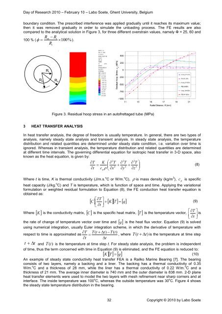
Day of Research 2010 – February 10 – Labo Soete, Ghent University, Belgium boundary condition. The prescribed interference was applied gradually until it reaches its maximum value; then it was removed gradually in order to simulate the unloading process. The FE results are also compared to the analytical solution in Figure 3, for three different overstrain values, namely Φ = 25, 60 and R R R m i 100 % ( 100% ). i R i R s R o Figure 3. Residual hoop stress in an autofrettaged tube (MPa) 3 HEAT TRANSFER ANALYSIS In heat transfer analysis, the degree of freedom is usually temperature. In general, there are two types of analysis, namely steady state analysis and transient analysis. In steady state analysis, the temperature distribution and related quantities are determined under steady state condition, i.e. variation over time is ignored. Whereas in transient analysis, the temperature distribution and related quantities are determined at different time intervals. The governing differential equation for isotropic heat transfer in 3-D space, also known as the heat equation, is given by: 2 2 2 T K T T T (8) 2 2 2 t cp x y z Where t is time, K is thermal conductivity (J/m.s. o C or W/m. o C), is mass density (kg/m 3 ), c p is specific heat capacity (J/kg. o C) and T is temperature, which is function of space and time. Applying the variational formulation or weighted residual formulation to Equation (8), the FE conduction heat transfer equation is obtained as: T C K T q (9) t Where K is the conductivity matrix, C is the specific heat matrix, T is the temperature vector, T is t the rate of change of temperature vector over time and q is the heat flux vector. Equation (9) is solved using numerical integration, usually Euler integration scheme, in which the derivative of temperature with respect to time is approximated as T T( t t) T( t ) , where T( t t) is the temperature at time step t t t t and T (t) is the temperature at time step t. For steady state analysis, the problem is independent of time, thus the term concerned with time in Equation (9) is eliminated, and the FE equation is reduced to: K T q (10) An example of steady state conductivity heat transfer FEA is a Railko Marine Bearing [7]. The bearing consists of two layers, namely a backing and a liner. The backing has a thermal conductivity of 0.35 W/m. o C and a thickness of 28 mm, while the liner has a thermal conductivity of 0.22 W/m. o C and a thickness of 21 mm. The average inner diameter is 740 mm and the outer diameter is 838 mm. 2-D plane heat transfer elements were used to model the two layers with mesh refinement near sharp corners and at interface. The inside temperature was 100 o C, whereas the outside temperature was 30 o C. Figure 4 shows the steady state temperature distribution in the bearing. 32 Copyright © 2010 by Labo Soete
Page 1: Day of Research 2010 - February 10
Page 5 and 6: Day of Research 2010 - February 10

F - 5th International Conference on Sustainable Construction and ...

You also want an ePaper? Increase the reach of your titles

Delete template?

Save as template?