Splitting the Unit Delay - IEEE Signal Processing ... - IEEE Xplore

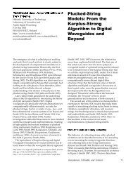
method but also irrespective of the amplitude curve approximated.This suggests that the Oetken method can be used tocontrol the delay of any FIR filter. This is, however, onlypossible when the zeros of the error function are knownbeforehand so that the transformation matrix (which onlydepends on the zeros) can be computed.3) Farrow Structure for Fractional Delay FIR FiltersA promising technique for efficient implementation of acontinuously variable delay element was proposed by Farrow[29]. This method assumes that the filter is designed off-line,but the real-time control of the delay value is simple andefficient. The basic idea is to design a set of filters approximatinga fractional delay in the desired range (e.g., 0s dG1) and then to approximate each coefficient as a Pth-orderpolynomial of d, or'. The Furrow structure for implementation of polynoimiul upproximationoffilter coeflcients.delay control Can be formulated as follows:1) Design a set of Q + 1 FIR filters of the (same) chosenorder N approximating in a desired sense the ideal nonintegerdelay whose fractional part takes values in the desired range[dmi,, dmax]. The values of d can be chosen, for example, on auniform grid as(59)where c,(n) are real-valued approximating coefficients. Thesubscript d is now included to emphasize that each coefficientis a function of the fractional delay, d. The transfer functionof the filter can be elaborated into the formThe result is the set of prototype filters with the coefficientshd,q(n) for q = 0, 1,2, ..., Q and n = 0, 1,2, ..., N.2) Design the polynomial structure approximating thecoefficients of the prototype filters in the desired sense so thatDhd,,(n) = xcm(n)d?, q = 0,1,2 ,..., Q; IZ = 0,1,2 ,..., Nm=O (63)where it was definedThe form (Eq. 60) immediately suggests an efficient implementationas a parallel connection of fixed filters withoutput taps weighted by an appropriate power of d (Fig. 7).The sample implementation presented in [29] was designedby employing least squared error criterion over thedesired frequency band and the employed range of d. Alsothe polynomial approximation of the filter coefficients wasdone in the least squares sense. An excellent tutorial presentationof the method with examples and performance analysisis included in [721, when applied to timing adjustment algorithmsin digital receivers.The polynomial approach can readily be generalized forother filter design techniques as well. In addition to the leastsquares method, maximally flat or equiripple approximationcan be employed to design the set of prototype filters coveringthe desired range of d. The coefficients of the filter set arethen approximated separately by the polynomial structure ofa desired order. Polynomial interpolation techniques, such asLagrange interpolation, can be realized using the Farrowstructure without further approximation [27], [ 1261, [130],[135].The design of the generalized polynomial structure forNote that the design reduces to L = N + 1 separate optimizationproblems: each polynomial approximation is carriedout for a fixed value of n. It is easiest to use least squares curvefitting for this task. According to our experience, second-orderpolynomials with three coefficients are usually sufficient.The resulting coefficients c,(n) are then employed to formthe transfer functions Cm(z) of the subsections, as shown inFig. 7.We applied the design method to imitate the response of4-tap equiripple approximations of Fig. A6. Second-orderpolynomials (P = 2) were used for coefficient approximation.The results are shown in Figs. 8a and 8b, which show thatboth the amplitude and phase delay characteristics are accuratelyreproduced, with hardly any observable deviation fromthe original ones (Figs. A6a and b). Similar results wereobtained for 10-tap filters. Farrow approximation with second-orderpolynomial approximation for coefficients thusprovides an accurate means for practical implementation ofFIR FD filters.The polynomial approximation technique can also be appliedto allpass filters, as will be discussed shortly.Summary of FIR Filter Design and ImplementationTo conclude our discussion of FIR FD filters, we present asummary of these techniques and evaluate their design complexity.As stated previously, our main interest is in faston-line tuning of the fractional delay and thus the fast updateof the coefficients is of paramount importance.JANUARY 1996 IEEE SIGNAL PROCESSING MAGAZINE 45