Calculus Made Easy, 2nd Edition

The Project Gutenberg EBook of Calculus Made Easy, by Silvanus ThompsonThis eBook is for the use of anyone anywhere at no cost and withalmost no restrictions whatsoever. You may copy it, give it away orre-use it under the terms of the Project Gutenberg License includedwith this eBook or online at www.gutenberg.orgTitle: Calculus Made EasyBeing a very-simplest introduction to those beautifulmethods which are generally called by the terrifying namesof the DifferentiaAuthor: Silvanus ThompsonRelease Date: October 9, 2012 [EBook #33283]Language: EnglishCharacter set encoding: ISO-8859-1*** START OF THIS PROJECT GUTENBERG EBOOK CALCULUS MADE EASY ***

Produced by Andrew D. Hwang, Brenda Lewis and the OnlineDistributed Proofreading Team at http://www.pgdp.net (Thisfile was produced from images generously made availableby The Internet Archive/American Libraries.)transcriber’s noteMinor presentational changes, and minor typographical andnumerical corrections, have been made without comment. Alltextual changes are detailed in the L A TEX source file.This PDF file is optimized for screen viewing, but may easily berecompiled for printing. Please see the preamble of the L A TEXsource file for instructions.

CALCULUS MADE EASY

MACMILLAN AND CO., LimitedLONDON : BOMBAY : CALCUTTAMELBOURNETHE MACMILLAN COMPANYNEW YORK : BOSTON : CHICAGODALLAS : SAN FRANCISCOTHE MACMILLAN CO. OF CANADA, Ltd.TORONTO

CALCULUS MADE EASY:BEING A VERY-SIMPLEST INTRODUCTION TOTHOSE BEAUTIFUL METHODS OF RECKONINGWHICH ARE GENERALLY CALLED BY THETERRIFYING NAMES OF THEDIFFERENTIAL CALCULUSAND THEINTEGRAL CALCULUS.BYF. R. S.SECOND EDITION, ENLARGEDMACMILLAN AND CO., LIMITEDST. MARTIN’S STREET, LONDON1914

COPYRIGHT.First Edition 1910.Reprinted 1911 (twice), 1912, 1913.Second Edition 1914.

What one fool can do, another can.(Ancient Simian Proverb.)

PREFACE TO THE SECOND EDITION.The surprising success of this work has led the author to add a considerablenumber of worked examples and exercises. Advantage hasalso been taken to enlarge certain parts where experience showed thatfurther explanations would be useful.The author acknowledges with gratitude many valuable suggestionsand letters received from teachers, students, and—critics.October, 1914.

viiCONTENTS.ChapterPagePrologue . . . . . . . . . . . . . . . . . . . . . . . . . . . . . . . . . . . . . . . ixI. To deliver you from the Preliminary Terrors 1II. On Different Degrees of Smallness . . . . . . . . . . . 3III. On Relative Growings . . . . . . . . . . . . . . . . . . . . . . . . . . 9IV. Simplest Cases . . . . . . . . . . . . . . . . . . . . . . . . . . . . . . . . . . 17V. Next Stage. What to do with Constants . . . . . . 25VI. Sums, Differences, Products and Quotients . . . 34VII. Successive Differentiation . . . . . . . . . . . . . . . . . . . . . 48VIII. When Time Varies . . . . . . . . . . . . . . . . . . . . . . . . . . . . . . 52IX. Introducing a Useful Dodge . . . . . . . . . . . . . . . . . . . 66X. Geometrical Meaning of Differentiation . . . . . . 75XI. Maxima and Minima . . . . . . . . . . . . . . . . . . . . . . . . . . . . . 91XII. Curvature of Curves . . . . . . . . . . . . . . . . . . . . . . . . . . . 109XIII. Other Useful Dodges . . . . . . . . . . . . . . . . . . . . . . . . . . 118XIV. On true Compound Interest and the Law of OrganicGrowth . . . . . . . . . . . . . . . . . . . . . . . . . . . . . 131

CALCULUS MADE EASYviiiChapterPageXV. How to deal with Sines and Cosines . . . . . . . . . . . 162XVI. Partial Differentiation . . . . . . . . . . . . . . . . . . . . . . . . 172XVII. Integration . . . . . . . . . . . . . . . . . . . . . . . . . . . . . . . . . . . . . 180XVIII. Integrating as the Reverse of Differentiating 189XIX. On Finding Areas by Integrating . . . . . . . . . . . . . . 204XX. Dodges, Pitfalls, and Triumphs . . . . . . . . . . . . . . . . 224XXI. Finding some Solutions . . . . . . . . . . . . . . . . . . . . . . . . . 232Table of Standard Forms . . . . . . . . . . . . . . . . . . . . . . . . 249Answers to Exercises. . . . . . . . . . . . . . . . . . . . . . . . . . . 252

PROLOGUE.Considering how many fools can calculate, it is surprising that itshould be thought either a difficult or a tedious task for any other foolto learn how to master the same tricks.Some calculus-tricks are quite easy. Some are enormously difficult.The fools who write the textbooks of advanced mathematics—and theyare mostly clever fools—seldom take the trouble to show you how easythe easy calculations are. On the contrary, they seem to desire toimpress you with their tremendous cleverness by going about it in themost difficult way.Being myself a remarkably stupid fellow, I have had to unteachmyself the difficulties, and now beg to present to my fellow fools theparts that are not hard. Master these thoroughly, and the rest willfollow. What one fool can do, another can.

CHAPTER I.TO DELIVER YOU FROM THE PRELIMINARYTERRORS.The preliminary terror, which chokes off most fifth-form boys fromeven attempting to learn how to calculate, can be abolished once forall by simply stating what is the meaning—in common-sense terms—ofthe two principal symbols that are used in calculating.These dreadful symbols are:(1) d which merely means “a little bit of.”Thus dx means a little bit of x; or du means a little bit of u. Ordinarymathematicians think it more polite to say “an element of,”instead of “a little bit of.” Just as you please. But you will find thatthese little ∫ bits (or elements) may be considered to be indefinitely small.(2) which is merely a long S, and may be called (if you like) “thesum of.” ∫∫Thus dx means the sum of all the little bits of x; or dt meansthe sum of all the little bits of t. Ordinary mathematicians call thissymbol “the integral of.” Now any fool can see that if x is consideredas made up of a lot of little bits, each of which is called dx, if youadd them all up together you get the sum of all the dx’s, (which is the

CALCULUS MADE EASY 2same thing as the whole of x). The word “integral” simply means “thewhole.” If you think of the duration of time for one hour, you may (ifyou like) think of it as cut up into 3600 little bits called seconds. Thewhole of the 3600 little bits added up together make one hour.When you see an expression that begins with this terrifying symbol,you will henceforth know that it is put there merely to give youinstructions that you are now to perform the operation (if you can) oftotalling up all the little bits that are indicated by the symbols thatfollow.That’s all.

CHAPTER II.ON DIFFERENT DEGREES OF SMALLNESS.We shall find that in our processes of calculation we have to deal withsmall quantities of various degrees of smallness.We shall have also to learn under what circumstances we may considersmall quantities to be so minute that we may omit them fromconsideration. Everything depends upon relative minuteness.Before we fix any rules let us think of some familiar cases. Thereare 60 minutes in the hour, 24 hours in the day, 7 days in the week.There are therefore 1440 minutes in the day and 10080 minutes in theweek.Obviously 1 minute is a very small quantity of time compared witha whole week. Indeed, our forefathers considered it small as comparedwith an hour, and called it “one minùte,” meaning a minutefraction—namely one sixtieth—of an hour. When they came to requirestill smaller subdivisions of time, they divided each minute into60 still smaller parts, which, in Queen Elizabeth’s days, they called“second minùtes” (i.e. small quantities of the second order of minuteness).Nowadays we call these small quantities of the second order ofsmallness “seconds.” But few people know why they are so called.Now if one minute is so small as compared with a whole day, how

CALCULUS MADE EASY 4much smaller by comparison is one second!Again, think of a farthing as compared with a sovereign: it is barelyworth more than 1 part. A farthing more or less is of precious little1000importance compared with a sovereign: it may certainly be regardedas a small quantity. But compare a farthing with £1000: relatively tothis greater sum, the farthing is of no more importance than 11000 of afarthing would be to a sovereign. Even a golden sovereign is relativelya negligible quantity in the wealth of a millionaire.Now if we fix upon any numerical fraction as constituting the proportionwhich for any purpose we call relatively small, we can easilystate other fractions of a higher degree of smallness. Thus if, for the11purpose of time, be called a small fraction, then of 1(being a60 60 60small fraction of a small fraction) may be regarded as a small quantityof the second order of smallness. ∗1Or, if for any purpose we were to take 1 per cent. (i.e. ) as a1001small fraction, then 1 per cent. of 1 per cent. (i.e. ) would be a10,0001small fraction of the second order of smallness; and would be1,000,000a small fraction of the third order of smallness, being 1 per cent. of1 per cent. of 1 per cent.Lastly, suppose that for some very precise purpose we should regard11,000,000as “small.” Thus, if a first-rate chronometer is not to loseor gain more than half a minute in a year, it must keep time withan accuracy of 1 part in 1, 051, 200. Now if, for such a purpose, we∗ The mathematicians talk about the second order of “magnitude” (i.e. greatness)when they really mean second order of smallness. This is very confusing tobeginners.

DIFFERENT DEGREES OF SMALLNESS 51regard (or one millionth) as a small quantity, then 1of1,000,000 1,000,0001, that is 1(or one billionth) will be a small quantity1,000,000 1,000,000,000,000of the second order of smallness, and may be utterly disregarded, bycomparison.Then we see that the smaller a small quantity itself is, the morenegligible does the corresponding small quantity of the second orderbecome. Hence we know that in all cases we are justified in neglectingthe small quantities of the second—or third (or higher)—orders, if onlywe take the small quantity of the first order small enough in itself.But, it must be remembered, that small quantities if they occur inour expressions as factors multiplied by some other factor, may becomeimportant if the other factor is itself large. Even a farthing becomesimportant if only it is multiplied by a few hundred.Now in the calculus we write dx for a little bit of x. These thingssuch as dx, and du, and dy, are called “differentials,” the differentialof x, or of u, or of y, as the case may be. [You read them as dee-eks,or dee-you, or dee-wy.] If dx be a small bit of x, and relatively small ofitself, it does not follow that such quantities as x · dx, or x 2 dx, or a x dxare negligible. But dx × dx would be negligible, being a small quantityof the second order.A very simple example will serve as illustration.Let us think of x as a quantity that can grow by a small amount soas to become x + dx, where dx is the small increment added by growth.The square of this is x 2 + 2x · dx + (dx) 2 .The second term is notnegligible because it is a first-order quantity; while the third term is ofthe second order of smallness, being a bit of, a bit of x 2 . Thus if we

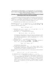
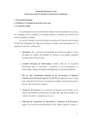
CALCULUS MADE EASY 61took dx to mean numerically, say, of x, then the second term would60be 2 of 60 x2 1, whereas the third term would be of 3600 x2 . This last termis clearly less important than the second. But if we go further and takedx to mean only 11000 of x, then the second term will be 21000 of x2 , whilethe third term will be only11,000,000 of x2 .xxFig. 1.Geometrically this may be depicted as follows:Draw a square(Fig. 1) the side of which we will take to represent x. Now supposethe square to grow by having a bit dx added to its size each way.The enlarged square is made up of the original square x 2 , the tworectangles at the top and on the right, each of which is of area x · dx(or together 2x · dx), and the little square at the top right-hand cornerwhich is (dx) 2 .In Fig. 2 we have taken dx as quite a big fractionof x—about 1 1. But suppose we had taken it only —about the5 100thickness of an inked line drawn with a fine pen. Then the little cornersquare will have an area of only110,000 of x2 , and be practically invisible.Clearly (dx) 2 is negligible if only we consider the increment dx to beitself small enough.Let us consider a simile.

DIFFERENT DEGREES OF SMALLNESS 7dxxdxdxx · dx (dx) 2xxx 2x · dxxdxFig. 2.Fig. 3.Suppose a millionaire were to say to his secretary: next week I willgive you a small fraction of any money that comes in to me. Supposethat the secretary were to say to his boy: I will give you a small fractionof what I get. Suppose the fraction in each case to be 1 part. Now100if Mr. Millionaire received during the next week £1000, the secretarywould receive £10 and the boy 2 shillings.Ten pounds would be asmall quantity compared with £1000; but two shillings is a small smallquantity indeed, of a very secondary order. But what would be thedisproportion if the fraction, instead of being 111000100, had been settled atpart? Then, while Mr. Millionaire got his £1000, Mr. Secretarywould get only £1, and the boy less than one farthing!The witty Dean Swift ∗ once wrote:“So, Nat’ralists observe, a Flea“Hath smaller Fleas that on him prey.“And these have smaller Fleas to bite ’em,“And so proceed ad infinitum.”∗ On Poetry: a Rhapsody (p. 20), printed 1733—usually misquoted.

CALCULUS MADE EASY 8An ox might worry about a flea of ordinary size—a small creature ofthe first order of smallness. But he would probably not trouble himselfabout a flea’s flea; being of the second order of smallness, it would benegligible. Even a gross of fleas’ fleas would not be of much account tothe ox.

CHAPTER III.ON RELATIVE GROWINGS.All through the calculus we are dealing with quantities that are growing,and with rates of growth. We classify all quantities into two classes:constants and variables. Those which we regard as of fixed value, andcall constants, we generally denote algebraically by letters from the beginningof the alphabet, such as a, b, or c; while those which we consideras capable of growing, or (as mathematicians say) of “varying,” we denoteby letters from the end of the alphabet, such as x, y, z, u, v, w,or sometimes t.Moreover, we are usually dealing with more than one variable atonce, and thinking of the way in which one variable depends on theother: for instance, we think of the way in which the height reachedby a projectile depends on the time of attaining that height. Or weare asked to consider a rectangle of given area, and to enquire how anyincrease in the length of it will compel a corresponding decrease in thebreadth of it. Or we think of the way in which any variation in theslope of a ladder will cause the height that it reaches, to vary.Suppose we have got two such variables that depend one on theother. An alteration in one will bring about an alteration in the other,because of this dependence. Let us call one of the variables x, and the

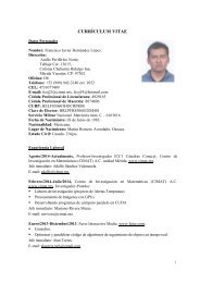
CALCULUS MADE EASY 10other that depends on it y.Suppose we make x to vary, that is to say, we either alter it orimagine it to be altered, by adding to it a bit which we call dx. We arethus causing x to become x + dx. Then, because x has been altered,y will have altered also, and will have become y + dy. Here the bit dymay be in some cases positive, in others negative; and it won’t (exceptby a miracle) be the same size as dx.Take two examples.(1) Let x and y be respectively the base and the height of a rightangledtriangle (Fig. 4), of which the slope of the other side is fixeddyyy30 ◦xFig. 4.dxat 30 ◦ . If we suppose this triangle to expand and yet keep its anglesthe same as at first, then, when the base grows so as to become x + dx,the height becomes y + dy. Here, increasing x results in an increaseof y. The little triangle, the height of which is dy, and the base of whichis dx, is similar to the original triangle; and it is obvious that the valueof the ratio dydx is the same as that of the ratio y . As the angle is 30◦xit will be seen that heredydx = 11.73 .

CALCULUS MADE EASY 12How much will y be diminished? The new height will be y − dy. Ifwe work out the height by Euclid I. 47, then we shall be able to findhow much dy will be. The length of the ladder is√(180)2 + (19) 2 = 181 inches.Clearly then, the new height, which is y − dy, will be such that(y − dy) 2 = (181) 2 − (20) 2 = 32761 − 400 = 32361,y − dy = √ 32361 = 179.89 inches.Now y is 180, so that dy is 180 − 179.89 = 0.11 inch.So we see that making dx an increase of 1 inch has resulted inmaking dy a decrease of 0.11 inch.And the ratio of dy to dx may be stated thus:dydx = −0.11 1 .It is also easy to see that (except in one particular position) dy willbe of a different size from dx.Now right through the differential calculus we are hunting, hunting,hunting for a curious thing, a mere ratio, namely, the proportion whichdy bears to dx when both of them are indefinitely small.It should be noted here that we can only find this ratio dydx wheny and x are related to each other in some way, so that whenever x variesy does vary also. For instance, in the first example just taken, if thebase x of the triangle be made longer, the height y of the trianglebecomes greater also, and in the second example, if the distance x ofthe foot of the ladder from the wall be made to increase, the height y

ON RELATIVE GROWINGS 13reached by the ladder decreases in a corresponding manner, slowly atfirst, but more and more rapidly as x becomes greater. In these casesthe relation between x and y is perfectly definite, it can be expressedmathematically, being y x = tan 30◦ and x 2 + y 2 = l 2 (where l is thelength of the ladder) respectively, and dy has the meaning we found indxeach case.If, while x is, as before, the distance of the foot of the ladder fromthe wall, y is, instead of the height reached, the horizontal length ofthe wall, or the number of bricks in it, or the number of years since itwas built, any change in x would naturally cause no change whateverin y; in this case dy has no meaning whatever, and it is not possibledxto find an expression for it. Whenever we use differentials dx, dy,dz, etc., the existence of some kind of relation between x, y, z, etc., isimplied, and this relation is called a “function” in x, y, z, etc.; the twoexpressions given above, for instance, namely y x = tan 30◦ and x 2 +y 2 =l 2 , are functions of x and y. Such expressions contain implicitly (thatis, contain without distinctly showing it) the means of expressing eitherx in terms of y or y in terms of x, and for this reason they are calledimplicit functions in x and y; they can be respectively put into theformsy = x tan 30 ◦ or x =ytan 30 ◦and y = √ l 2 − x 2 or x = √ l 2 − y 2 .These last expressions state explicitly (that is, distinctly) the valueof x in terms of y, or of y in terms of x, and they are for this reasoncalled explicit functions of x or y. For example x 2 + 3 = 2y − 7 is an

CALCULUS MADE EASY 14implicit function in x and y; it may be written y = x2 + 10(explicit2function of x) or x = √ 2y − 10 (explicit function of y). We see thatan explicit function in x, y, z, etc., is simply something the value ofwhich changes when x, y, z, etc., are changing, either one at the timeor several together. Because of this, the value of the explicit functionis called the dependent variable, as it depends on the value of the othervariable quantities in the function; these other variables are called theindependent variables because their value is not determined from thevalue assumed by the function. For example, if u = x 2 sin θ, x and θare the independent variables, and u is the dependent variable.Sometimes the exact relation between several quantities x, y, z eitheris not known or it is not convenient to state it; it is only known,or convenient to state, that there is some sort of relation between thesevariables, so that one cannot alter either x or y or z singly withoutaffecting the other quantities; the existence of a function in x, y, zis then indicated by the notation F (x, y, z) (implicit function) or byx = F (y, z), y = F (x, z) or z = F (x, y) (explicit function). Sometimesthe letter f or φ is used instead of F , so that y = F (x), y = f(x) andy = φ(x) all mean the same thing, namely, that the value of y dependson the value of x in some way which is not stated.We call the ratio dy “the differential coefficient of y with respectdxto x.” It is a solemn scientific name for this very simple thing. Butwe are not going to be frightened by solemn names, when the thingsthemselves are so easy. Instead of being frightened we will simply pronouncea brief curse on the stupidity of giving long crack-jaw names;and, having relieved our minds, will go on to the simple thing itself,

ON RELATIVE GROWINGS 15namely the ratio dydx .In ordinary algebra which you learned at school, you were alwayshunting after some unknown quantity which you called x or y; or sometimesthere were two unknown quantities to be hunted for simultaneously.You have now to learn to go hunting in a new way; the fox beingnow neither x nor y. Instead of this you have to hunt for this curiouscub called dydy. The process of finding the value of is called “differentiating.”But, remember, what is wanted is the value of thisdx dxratiowhen both dy and dx are themselves indefinitely small. The true valueof the differential coefficient is that to which it approximates in thelimiting case when each of them is considered as infinitesimally minute.Let us now learn how to go in quest of dydx .

CALCULUS MADE EASY 16NOTE TO CHAPTER III.How to read Differentials.It will never do to fall into the schoolboy error of thinking that dxmeans d times x, for d is not a factor—it means “an element of” or “abit of” whatever follows. One reads dx thus: “dee-eks.”In case the reader has no one to guide him in such matters it mayhere be simply said that one reads differential coefficients in the followingway. The differential coefficientSo alsodydxis read “dee-wy by dee-eks,” or “dee-wy over dee-eks.”dudtis read “dee-you by dee-tee.”Second differential coefficients will be met with later on. They arelike this:d 2 y; which is read “dee-two-wy over dee-eks-squared,”dx2 and it means that the operation of differentiating y with respect to xhas been (or has to be) performed twice over.Another way of indicating that a function has been differentiated isby putting an accent to the symbol of the function. Thus if y = F (x),which means that y is some unspecified function of x (see p. 13), we maywrite F ′ (x) instead of d( F (x) ). Similarly, F ′′ (x) will mean that thedxoriginal function F (x) has been differentiated twice over with respectto x.

CHAPTER IV.SIMPLEST CASES.Now let us see how, on first principles, we can differentiate some simplealgebraical expression.Case 1.Let us begin with the simple expression y = x 2 . Now rememberthat the fundamental notion about the calculus is the idea of growing.Mathematicians call it varying. Now as y and x 2 are equal to oneanother, it is clear that if x grows, x 2 will also grow. And if x 2 grows,then y will also grow. What we have got to find out is the proportionbetween the growing of y and the growing of x. In other words our taskis to find out the ratio between dy and dx, or, in brief, to find the valueof dydx .Let x, then, grow a little bit bigger and become x + dx; similarly,y will grow a bit bigger and will become y+dy. Then, clearly, it will stillbe true that the enlarged y will be equal to the square of the enlarged x.Writing this down, we have:y + dy = (x + dx) 2 .

SIMPLEST CASES 19Numerical example.Suppose x = 100 and ∴ y = 10, 000. Then let x grow till it becomes101 (that is, let dx = 1). Then the enlarged y will be 101 × 101 =10, 201. But if we agree that we may ignore small quantities of thesecond order, 1 may be rejected as compared with 10, 000; so we mayround off the enlarged y to 10, 200. y has grown from 10, 000 to 10, 200;the bit added on is dy, which is therefore 200.dydx = 200 = 200. According to the algebra-working of the previous1paragraph, we find dy = 2x. And so it is; for x = 100 and 2x = 200.dxBut, you will say, we neglected a whole unit.Well, try again, making dx a still smaller bit.Try dx = 1 . Then x + dx = 100.1, and10(x + dx) 2 = 100.1 × 100.1 = 10, 020.01.Now the last figure 1 is only one-millionth part of the 10, 000, andis utterly negligible; so we may take 10, 020 without the little decimalat the end. And this makes dy = 20; and dydx = 20 = 200, which is0.1still the same as 2x.Case 2.Try differentiating y = x 3 in the same way.We let y grow to y + dy, while x grows to x + dx.Then we havey + dy = (x + dx) 3 .Doing the cubing we obtainy + dy = x 3 + 3x 2 · dx + 3x(dx) 2 + (dx) 3 .

CALCULUS MADE EASY 20Now we know that we may neglect small quantities of the secondand third orders; since, when dy and dx are both made indefinitelysmall, (dx) 2 and (dx) 3 will become indefinitely smaller by comparison.So, regarding them as negligible, we have left:y + dy = x 3 + 3x 2 · dx.But y = x 3 ; and, subtracting this, we have:anddy = 3x 2 · dx,dydx = 3x2 .Case 3.Try differentiating y = x 4 . Starting as before by letting both y and xgrow a bit, we have:y + dy = (x + dx) 4 .Working out the raising to the fourth power, we gety + dy = x 4 + 4x 3 dx + 6x 2 (dx) 2 + 4x(dx) 3 + (dx) 4 .Then striking out the terms containing all the higher powers of dx,as being negligible by comparison, we havey + dy = x 4 + 4x 3 dx.Subtracting the original y = x 4 , we have leftanddy = 4x 3 dx,dydx = 4x3 .

SIMPLEST CASES 21Now all these cases are quite easy. Let us collect the results to see ifwe can infer any general rule. Put them in two columns, the values of yin one and the corresponding values found for dy in the other: thusdxyx 2dydx2xx 3 3x 2x 4 4x 3Just look at these results: the operation of differentiating appearsto have had the effect of diminishing the power of x by 1 (for examplein the last case reducing x 4 to x 3 ), and at the same time multiplying bya number (the same number in fact which originally appeared as thepower). Now, when you have once seen this, you might easily conjecturehow the others will run. You would expect that differentiating x 5 wouldgive 5x 4 , or differentiating x 6 would give 6x 5 . If you hesitate, try oneof these, and see whether the conjecture comes right.Try y = x 5 .Then y + dy = (x + dx) 5= x 5 + 5x 4 dx + 10x 3 (dx) 2 + 10x 2 (dx) 3+ 5x(dx) 4 + (dx) 5 .Neglecting all the terms containing small quantities of the higherorders, we have lefty + dy = x 5 + 5x 4 dx,

SIMPLEST CASES 23Expanding this by the binomial theorem (see p. 137), we get[= x −2 1 − 2 dx( ) 22(2 + 1) dx+ − etc.]x 1 × 2 xhave:= x −2 − 2x −3 · dx + 3x −4 (dx) 2 − 4x −5 (dx) 3 + etc.So, neglecting the small quantities of higher orders of smallness, wey + dy = x −2 − 2x −3 · dx.Subtracting the original y = x −2 , we finddy = −2x −3 dx,dydx = −2x−3 .And this is still in accordance with the rule inferred above.Case of a fractional power.Let y = x 1 2 . Then, as before,(y + dy = (x + dx) 1 12 = x 2 1 + dx ) 12x= √ x + 1 dx√ − 1 2 x 8(dx) 2x √ x + terms with higherpowers of dx.Subtracting the original y = x 1 2 , and neglecting higher powers wehave left:dy = 1 dx√ = 1 12 x 2 x− 2 · dx,

CALCULUS MADE EASY 24and dydx = 1 2 x− 1 2 . Agreeing with the general rule.Summary. Let us see how far we have got. We have arrived at thefollowing rule: To differentiate x n , multiply by the power and reducethe power by one, so giving us nx n−1 as the result.Exercises I.Differentiate the following:(See p. 252 for Answers.)(1) y = x 13 (2) y = x − 3 2(3) y = x 2a (4) u = t 2.4(5) z = 3√ u (6) y = 3√ x −5(7) u = 5 √1x 8 (8) y = 2x a(9) y = q√ x 3 (10) y = n √1x mis!You have now learned how to differentiate powers of x. How easy it

CHAPTER V.NEXT STAGE. WHAT TO DO WITH CONSTANTS.In our equations we have regarded x as growing, and as a result of xbeing made to grow y also changed its value and grew. We usuallythink of x as a quantity that we can vary; and, regarding the variationof x as a sort of cause, we consider the resulting variation of y as aneffect. In other words, we regard the value of y as depending on thatof x. Both x and y are variables, but x is the one that we operate upon,and y is the “dependent variable.” In all the preceding chapter we havebeen trying to find out rules for the proportion which the dependentvariation in y bears to the variation independently made in x.Our next step is to find out what effect on the process of differentiatingis caused by the presence of constants, that is, of numbers whichdon’t change when x or y change their values.Added Constants.Let us begin with some simple case of an added constant, thus:Let y = x 3 + 5.Just as before, let us suppose x to grow to x+dx and y to grow to y+dy.

CALCULUS MADE EASY 26Then: y + dy = (x + dx) 3 + 5= x 3 + 3x 2 dx + 3x(dx) 2 + (dx) 3 + 5.Neglecting the small quantities of higher orders, this becomesy + dy = x 3 + 3x 2 · dx + 5.Subtract the original y = x 3 + 5, and we have left:dy = 3x 2 dx.dydx = 3x2 .So the 5 has quite disappeared.It added nothing to the growthof x, and does not enter into the differential coefficient. If we had put 7,or 700, or any other number, instead of 5, it would have disappeared.So if we take the letter a, or b, or c to represent any constant, it willsimply disappear when we differentiate.If the additional constant had been of negative value, such as−5 or −b, it would equally have disappeared.Multiplied Constants.Take as a simple experiment this case:Let y = 7x 2 .Then on proceeding as before we get:y + dy = 7(x + dx) 2= 7{x 2 + 2x · dx + (dx) 2 }= 7x 2 + 14x · dx + 7(dx) 2 .

CALCULUS MADE EASY 30Squaring, we get(a − b) 2 y 2 + (a + b) 2 x 2 + 2(a + b)(a − b)xy = (x 2 + y 2 + 2xy)(a 2 − b 2 ),which simplifies to(a − b) 2 y 2 + (a + b) 2 x 2 = x 2 (a 2 − b 2 ) + y 2 (a 2 − b 2 );or [(a − b) 2 − (a 2 − b 2 )]y 2 = [(a 2 − b 2 ) − (a + b) 2 ]x 2 ,that is 2b(b − a)y 2 = −2b(b + a)x 2 ;hence y =√a + ba − b x and dydx = √a + ba − b .(4) The volume of a cylinder of radius r and height h is given bythe formula V = πr 2 h. Find the rate of variation of volume with theradius when r = 5.5 in. and h = 20 in. If r = h, find the dimensionsof the cylinder so that a change of 1 in. in radius causes a change of400 cub. in. in the volume.The rate of variation of V with regard to r isdVdr = 2πrh.If r = 5.5 in. and h = 20 in. this becomes 690.8.It meansthat a change of radius of 1 inch will cause a change of volume of690.8 cub. inch. This can be easily verified, for the volumes withr = 5 and r = 6 are 1570 cub. in. and 2260.8 cub. in. respectively, and2260.8 − 1570 = 690.8.Also, ifr = h,√dV400dr = 2πr2 = 400 and r = h =2π= 7.98 in.

WHAT TO DO WITH CONSTANTS 31(5) The reading θ of a Féry’s Radiation pyrometer is related to theCentigrade temperature t of the observed body by the relation( ) 4θ t= ,θ 1 t 1where θ 1 is the reading corresponding to a known temperature t 1 of theobserved body.Compare the sensitiveness of the pyrometer at temperatures800 ◦ C., 1000 ◦ C., 1200 ◦ C., given that it read 25 when the temperaturewas 1000 ◦ C.The sensitiveness is the rate of variation of the reading with thetemperature, that is dθ . The formula may be writtendtand we haveθ = θ 1t 4 = 25t4t 4 1 1000 , 4dθdt = 100t31000 4 = t 310, 000, 000, 000 .When t = 800, 1000 and 1200, we get dθ = 0.0512, 0.1 and 0.1728dtrespectively.The sensitiveness is approximately doubled from 800 ◦ to 1000 ◦ , andbecomes three-quarters as great again up to 1200 ◦ .Exercises II. (See p. 252 for Answers.)Differentiate the following:(1) y = ax 3 + 6. (2) y = 13x 2 3 − c.

CALCULUS MADE EASY 32(3) y = 12x 1 2 + c 1 2 . (4) y = c 1 2 x 1 2 .(5) u = azn − 1. (6) y = 1.18t 2 + 22.4.cMake up some other examples for yourself, and try your hand atdifferentiating them.(7) If l t and l 0 be the lengths of a rod of iron at the temperaturest ◦ C. and 0 ◦ C. respectively, then l t = l 0 (1+0.000012t). Find the changeof length of the rod per degree Centigrade.(8) It has been found that if c be the candle power of an incandescentelectric lamp, and V be the voltage, c = aV b , where a and b areconstants.Find the rate of change of the candle power with the voltage, andcalculate the change of candle power per volt at 80, 100 and 120 voltsin the case of a lamp for which a = 0.5 × 10 −10 and b = 6.(9) The frequency n of vibration of a string of diameter D, length Land specific gravity σ, stretched with a force T , is given byn = 1√gTDL πσ .Find the rate of change of the frequency when D, L, σ and T arevaried singly.(10) The greatest external pressure P which a tube can support withoutcollapsing is given byP =( 2E1 − σ 2 ) t3D 3 ,

WHAT TO DO WITH CONSTANTS 33where E and σ are constants, t is the thickness of the tube and D isits diameter. (This formula assumes that 4t is small compared to D.)Compare the rate at which P varies for a small change of thicknessand for a small change of diameter taking place separately.(11) Find, from first principles, the rate at which the following varywith respect to a change in radius:(a) the circumference of a circle of radius r;(b) the area of a circle of radius r;(c) the lateral area of a cone of slant dimension l;(d) the volume of a cone of radius r and height h;(e) the area of a sphere of radius r;(f ) the volume of a sphere of radius r.(12) The length L of an iron rod at the temperature T being given by[ ]L = l t 1+0.000012(T −t) , where lt is the length at the temperature t,find the rate of variation of the diameter D of an iron tyre suitable forbeing shrunk on a wheel, when the temperature T varies.

CHAPTER VI.SUMS, DIFFERENCES, PRODUCTS ANDQUOTIENTS.We have learned how to differentiate simple algebraical functions suchas x 2 + c or ax 4 , and we have now to consider how to tackle the sumof two or more functions.For instance, lety = (x 2 + c) + (ax 4 + b);what will its dy be? How are we to go to work on this new job?dxThe answer to this question is quite simple: just differentiate them,one after the other, thus:dydx = 2x + 4ax3 .(Ans.)If you have any doubt whether this is right, try a more general case,working it by first principles. And this is the way.Let y = u+v, where u is any function of x, and v any other functionof x. Then, letting x increase to x + dx, y will increase to y + dy; andu will increase to u + du; and v to v + dv.And we shall have:y + dy = u + du + v + dv.

SUMS, DIFFERENCES, PRODUCTS 35Subtracting the original y = u + v, we getdy = du + dv,and dividing through by dx, we get:dydx = dudx + dvdx .This justifies the procedure. You differentiate each function separatelyand add the results.So if now we take the example of thepreceding paragraph, and put in the values of the two functions, weshall have, using the notation shown (p. 16),exactly as before.thatdydx = d(x2 + c)+ d(ax4 + b)dx dx= 2x + 4ax 3 ,If there were three functions of x, which we may call u, v and w, sotheny = u + v + w;dydx = dudx + dvdx + dwdx .As for subtraction, it follows at once; for if the function v had itselfhad a negative sign, its differential coefficient would also be negative;so that by differentiatingwe should gety = u − v,dydx = dudx − dvdx .

CALCULUS MADE EASY 36But when we come to do with Products, the thing is not quite sosimple.Suppose we were asked to differentiate the expressiony = (x 2 + c) × (ax 4 + b),what are we to do? The result will certainly not be 2x × 4ax 3 ; for itis easy to see that neither c × ax 4 , nor x 2 × b, would have been takeninto that product.Now there are two ways in which we may go to work.First way. Do the multiplying first, and, having worked it out, thendifferentiate.Accordingly, we multiply together x 2 + c and ax 4 + b.This gives ax 6 + acx 4 + bx 2 + bc.Now differentiate, and we get:dydx = 6ax5 + 4acx 3 + 2bx.Second way. Go back to first principles, and consider the equationy = u × v;where u is one function of x, and v is any other function of x. Then, ifx grows to be x + dx; and y to y + dy; and u becomes u + du, and vbecomes v + dv, we shall have:y + dy = (u + du) × (v + dv)= u · v + u · dv + v · du + du · dv.

SUMS, DIFFERENCES, PRODUCTS 37Now du·dv is a small quantity of the second order of smallness, andtherefore in the limit may be discarded, leavingy + dy = u · v + u · dv + v · du.Then, subtracting the original y = u · v, we have leftdy = u · dv + v · du;and, dividing through by dx, we get the result:dydx = u dvdx + v dudx .This shows that our instructions will be as follows: To differentiatethe product of two functions, multiply each function by the differentialcoefficient of the other, and add together the two products so obtained.You should note that this process amounts to the following: Treat uas constant while you differentiate v; then treat v as constant while youdifferentiate u; and the whole differential coefficient dy will be the sumdxof these two treatments.Now, having found this rule, apply it to the concrete example whichwas considered above.We want to differentiate the product(x 2 + c) × (ax 4 + b).Call (x 2 + c) = u; and (ax 4 + b) = v.

CALCULUS MADE EASY 38Then, by the general rule just established, we may write:exactly as before.dydx = (x2 + c) d(ax4 + b)+ (ax 4 + b) d(x2 + c)dxdx= (x 2 + c) 4ax 3 + (ax 4 + b) 2x= 4ax 5 + 4acx 3 + 2ax 5 + 2bx,dydx = 6ax5 + 4acx 3+ 2bx,Lastly, we have to differentiate quotients.Think of this example, y = bx5 + c. In such a case it is no use tox 2 + atry to work out the division beforehand, because x 2 + a will not divideinto bx 5 + c, neither have they any common factor. So there is nothingfor it but to go back to first principles, and find a rule.So we will put y = u v ;where u and v are two different functions of the independent variable x.Then, when x becomes x + dx, y will become y + dy; and u will becomeu + du; and v will become v + dv. So theny + dy = u + duv + dv .

QUOTIENTS 39Now perform the algebraic division, thus:v + dvu + duu + u · dvvdu − u · dvvdu · dvdu +v− u · dvv− u · dvvuv + du v − u · dvv 2du · dv−v−−u · dv · dvv 2du · dvv+u · dv · dvv 2 .As both these remainders are small quantities of the second order,they may be neglected, and the division may stop here, since any furtherremainders would be of still smaller magnitudes.So we have got:which may be writteny + dy = u v + du v − u · dvv 2 ;= u v+v · du − u · dvv 2 .

CALCULUS MADE EASY 40Now subtract the original y = u , and we have left:vwhencev · du − u · dvdy = ;v 2dy v dudx = dx − u dvdx .v 2This gives us our instructions as to how to differentiate a quotientof two functions. Multiply the divisor function by the differential coefficientof the dividend function; then multiply the dividend function bythe differential coefficient of the divisor function; and subtract. Lastlydivide by the square of the divisor function.Going back to our example y = bx5 + cx 2 + a ,write bx 5 + c = u;and x 2 + a = v.Thendy (x 2 + a) d(bx5 + c)− (bx 5 + c) d(x2 + a)dx = dxdx(x 2 + a) 2= (x2 + a)(5bx 4 ) − (bx 5 + c)(2x),(x 2 + a) 2dydx = 3bx6 + 5abx 4 − 2cx. (Answer.)(x 2 + a) 2The working out of quotients is often tedious, but there is nothingdifficult about it.Some further examples fully worked out are given hereafter.

DIFFERENTIATION 41(1) Differentiate y = a b 2 x3 − a2b x + a2b 2 .Being a constant, a2b 2vanishes, and we havedydx = a b 2 × 3 × x3−1 − a2b × 1 × x1−1 .But x 1−1 = x 0 = 1; so we get:dydx = 3ab 2 x2 − a2b .(2) Differentiate y = 2a √ bx 3 − 3b 3√ a− 2 √ ab.xPutting x in the index form, we gety = 2a √ bx 3 2 − 3b3 √ ax −1 − 2 √ ab.or,Nowdydx = 2a√ b × 3 × x 2 3 −1 − 3b 3√ a × (−1) × x −1−1 ;2dydx = 3a√ bx + 3b 3√ a.x 2or,or,(3) Differentiate z = 1.8 3 √1θ 2 − 4.45√θ− 27 ◦ .This may be written: z = 1.8 θ − 2 3 − 4.4 θ − 1 5 − 27 ◦ .The 27 ◦ vanishes, and we havedzdθ = 1.8 × − 2 × 2 3 θ− 3 −1 − 4.4 × ( )− 1 5 θ− 1 5 −1 ;dzdθ = −1.2 5 θ− 3 + 0.88 θ− 6 5 ;dzdθ = 0.885√ − 1.2θ6 3√ .θ5

CALCULUS MADE EASY 42(4) Differentiate v = (3t 2 − 1.2t + 1) 3 .A direct way of doing this will be explained later (see p. 66); butwe can nevertheless manage it now without any difficulty.henceDeveloping the cube, we getv = 27t 6 − 32.4t 5 + 39.96t 4 − 23.328t 3 − 13.32t 2 − 3.6t + 1;dvdt = 162t5 − 162t 4 + 159.84t 3 − 69.984t 2 + 26.64t − 3.6.(5) Differentiate y = (2x − 3)(x + 1) 2 .dydx = (2x − 3) d[ (x + 1)(x + 1) ][ dx= (2x − 3) (x + 1)d(x + 1)dx2 d(2x − 3)+ (x + 1)dx ]+ (x + 1)d(x + 1)dx2 d(2x − 3)+ (x + 1)dx= 2(x + 1) [ (2x − 3) + (x + 1) ] = 2(x + 1)(3x − 2);or, more simply, multiply out and then differentiate.(6) Differentiate y = 0.5x 3 (x − 3).[]dydx = 0.5 3 d(x − 3)x + (x − 3) d(x3 )dxdx= 0.5 [ x 3 + (x − 3) × 3x 2] = 2x 3 − 4.5x 2 .Same remarks as for preceding ( example.(7) Differentiate w = θ + 1 ) ( ) √θ 1 + √θ .θ

DIFFERENTIATION 43This may be writtenw = (θ + θ −1 )(θ 1 2 + θ− 1 2 ).dwdθ = (θ + θ−1 ) d(θ 1 2 + θ − 2 1 )+ (θ 1 2 + θ− 1 d(θ + θ −1 )2 )dθdθ= (θ + θ −1 )( 1 2 θ− 1 2 −12 θ− 3 2 ) + (θ12 + θ− 1 2 )(1 − θ −2 )= 1(θ 1 22 + θ− 2 3 − θ− 1 2 − θ− 2 5 1) + (θ 2 + θ− 1 2 − θ− 3 2 − θ− 5 2 )( ) ( √θ= 3 1 1√θ2 − √ + 1 − 1 )√ .θ5 2 θ3This, again, could be obtained more simply by multiplying the twofactors first, and differentiating afterwards. This is not, however, alwayspossible; see, for instance, p. 170, example 8, in which the rule fordifferentiating a product must be used.a(8) Differentiate y =1 + a √ x + a 2 x .dy (1 + ax 1 2 + a 2 x) × 0 − a d(1 + ax 1 2 + a 2 x)dx = dx(1 + a √ x + a 2 x) 2= − a( 1 2 ax− 1 2 + a 2 )(1 + ax 1 2 + a 2 x) 2 .(9) Differentiate y = x2x 2 + 1 .dydx = (x2 + 1) 2x − x 2 × 2x(x 2 + 1) 2 =(10) Differentiate y = a + √ xa − √ x .2x(x 2 + 1) 2 .

CALCULUS MADE EASY 44In the indexed form, y = a + x 1 2.a − x 1 2dydx = (a − x 1 2 )( 1 2 x− 2 1 ) − (a + x 1 2 )(− 1 2 x− 1 2 )= a − x 1 2 + a + x 1 2;(a − x 2 1 ) 2 2(a − x 1 2 ) 2 x 1 2dyhencedx = a(a − √ x) √ 2 x .(11) Differentiate θ = 1 − a 3√ t 21 + a 2√ t 3 .Now θ = 1 − at 32 .1 + at 3 2dθdt = (1 + at 3 2 )(− 2 3 at− 1 3 ) − (1 − at 2 3 ) × 3 2 at 1 2(1 + at 3 2 ) 2=5a 2 6√ t 7 − 4a3√t− 9a 2√ t6(1 + a 2√ t 3 ) 2 .(12) A reservoir of square cross-section has sides sloping at an angleof 45 ◦ with the vertical. The side of the bottom is 200 feet. Find anexpression for the quantity pouring in or out when the depth of watervaries by 1 foot; hence find, in gallons, the quantity withdrawn hourlywhen the depth is reduced from 14 to 10 feet in 24 hours.The volume of a frustum of pyramid of height H, and of bases Aand a, is V = H 3 (A + a + √ Aa). It is easily seen that, the slope being45 ◦ , if the depth be h, the length of the side of the square surface ofthe water is 200 + 2h feet, so that the volume of water ish3 [2002 + (200 + 2h) 2 + 200(200 + 2h)] = 40, 000h + 400h 2 + 4h33 .

DIFFERENTIATION 45dVdh = 40, 000 + 800h + 4h2 = cubic feet per foot of depth variation.dVThe mean level from 14 to 10 feet is 12 feet, when h = 12,dh =50, 176 cubic feet.Gallons per hour corresponding to a change of depth of 4 ft. in4 × 50, 176 × 6.2524 hours = = 52, 267 gallons.24(13) The absolute pressure, in atmospheres, P , of saturated steam( ) 5 40 + tat the temperature t ◦ C. is given by Dulong as being P =140as long as t is above 80 ◦ . Find the rate of variation of the pressure withthe temperature at 100 ◦ C.Expand the numerator by the binomial theorem (see p. 137).P = 1140 5 (405 + 5 × 40 4 t + 10 × 40 3 t 2 + 10 × 40 2 t 3 + 5 × 40t 4 + t 5 );hencedPdt = 1537, 824 × 10 5(5 × 40 4 + 20 × 40 3 t + 30 × 40 2 t 2 + 20 × 40t 3 + 5t 4 ),when t = 100 this becomes 0.036 atmosphere per degree Centigradechange of temperature.Exercises III. (See the Answers on p. 253.)(1) Differentiate(a) u = 1 + x +x21 × 2 + x 31 × 2 × 3 + · · · .(b) y = ax 2 + bx + c. (c) y = (x + a) 2 .(d) y = (x + a) 3 .

CALCULUS MADE EASY 46(2) If w = at − 1 2 bt2 , find dwdt .(3) Find the differential coefficient ofy = (x + √ −1) × (x − √ −1).(4) Differentiatey = (197x − 34x 2 ) × (7 + 22x − 83x 3 ).(5) If x = (y + 3) × (y + 5), find dxdy .(6) Differentiate y = 1.3709x × (112.6 + 45.202x 2 ).Find the differential coefficients of(7) y = 2x + 33x + 2 . (8) y = 1 + x + 2x2 + 3x 31 + x + 2x 2 .(9) y = ax + bcx + d .(10) y = xn + ax −n + b .(11) The temperature t of the filament of an incandescent electriclamp is connected to the current passing through the lamp by the relationC = a + bt + ct 2 .Find an expression giving the variation of the current correspondingto a variation of temperature.(12) The following formulae have been proposed to express the relationbetween the electric resistance R of a wire at the temperature

DIFFERENTIATION 47t ◦ C., and the resistance R 0 of that same wire at 0 ◦ Centigrade, a, b, cbeing constants.R = R 0 (1 + at + bt 2 ).R = R 0 (1 + at + b √ t).R = R 0 (1 + at + bt 2 ) −1 .Find the rate of variation of the resistance with regard to temperatureas given by each of these formulae.(13) The electromotive-force E of a certain type of standard cell hasbeen found to vary with the temperature t according to the relationE = 1.4340 [ 1 − 0.000814(t − 15) + 0.000007(t − 15) 2] volts.Find the change of electromotive-force per degree, at 15 ◦ , 20 ◦and 25 ◦ .(14) The electromotive-force necessary to maintain an electric arc oflength l with a current of intensity i has been found by Mrs. Ayrton tobewhere a, b, c, k are constants.E = a + bl + c + kl ,iFind an expression for the variation of the electromotive-force(a) with regard to the length of the arc; (b) with regard to the strengthof the current.

CHAPTER VII.SUCCESSIVE DIFFERENTIATION.Let us try the effect of repeating several times over the operation ofdifferentiating a function (see p. 13). Begin with a concrete case.Let y = x 5 .First differentiation, 5x 4 .Second differentiation, 5 × 4x 3 = 20x 3 .Third differentiation, 5 × 4 × 3x 2 = 60x 2 .Fourth differentiation, 5 × 4 × 3 × 2x = 120x.Fifth differentiation, 5 × 4 × 3 × 2 × 1 = 120.Sixth differentiation, = 0.There is a certain notation, with which we are already acquainted(see p. 14), used by some writers, that is very convenient. This isto employ the general symbol f(x) for any function of x. Here thesymbol f( ) is read as “function of,” without saying what particularfunction is meant. So the statement y = f(x) merely tells us that y isa function of x, it may be x 2 or ax n , or cos x or any other complicatedfunction of x.

SUCCESSIVE DIFFERENTIATION 49The corresponding symbol for the differential coefficient is f ′ (x),which is simpler to write than dy . This is called the “derived function”dxof x.Suppose we differentiate over again, we shall get the “second derivedfunction” or second differential coefficient, which is denoted by f ′′ (x);and so on.For,Now let us generalize.Let y = f(x) = x n .First differentiation, f ′ (x) = nx n−1 .Second differentiation, f ′′ (x) = n(n − 1)x n−2 .Third differentiation, f ′′′ (x) = n(n − 1)(n − 2)x n−3 .Fourth differentiation, f ′′′′ (x) = n(n − 1)(n − 2)(n − 3)x n−4 .etc., etc.But this is not the only way of indicating successive differentiations.if the original function bey = f(x);dyonce differentiating givesdx = f ′ (x);( ) dyddxtwice differentiating gives= f ′′ (x);dxd 2 yand this is more conveniently written as(dx) , or more usually d2 y2 dx . 2Similarly, we may write as the result of thrice differentiating, d3 ydx 3 =f ′′′ (x).

CALCULUS MADE EASY 50Examples.Now let us try y = f(x) = 7x 4 + 3.5x 3 − 1 2 x2 + x − 2.dydx = f ′ (x) = 28x 3 + 10.5x 2 − x + 1,d 2 ydx 2 = f ′′ (x) = 84x 2 + 21x − 1,d 3 ydx 3 = f ′′′ (x) = 168x + 21,d 4 ydx 4 = f ′′′′ (x) = 168,d 5 ydx 5 = f ′′′′′ (x) = 0.In a similar manner if y = φ(x) = 3x(x 2 − 4),φ ′ (x) = dydx = 3[ x × 2x + (x 2 − 4) × 1 ] = 3(3x 2 − 4),φ ′′ (x) = d2 y= 3 × 6x = 18x,dx2 φ ′′′ (x) = d3 ydx = 18, 3φ ′′′′ (x) = d4 ydx = 0. 4Exercises IV. (See page 253 for Answers.)Find dydx and d2 yfor the following expressions:dx2 (1) y = 17x + 12x 2 .(2) y = x2 + ax + a .(3) y = 1 + x 1 + x21 × 2 + x 31 × 2 × 3 + x 41 × 2 × 3 × 4 .

SUCCESSIVE DIFFERENTIATION 51(4) Find the 2nd and 3rd derived functions in the Exercises III.(p. 45), No. 1 to No. 7, and in the Examples given (p. 40), No. 1 toNo. 7.

CHAPTER VIII.WHEN TIME VARIES.Some of the most important problems of the calculus are those wheretime is the independent variable, and we have to think about the valuesof some other quantity that varies when the time varies. Some thingsgrow larger as time goes on; some other things grow smaller. The distancethat a train has got from its starting place goes on ever increasingas time goes on. Trees grow taller as the years go by. Which is growingat the greater rate; a plant 12 inches high which in one month becomes14 inches high, or a tree 12 feet high which in a year becomes 14 feethigh?In this chapter we are going to make much use of the word rate.Nothing to do with poor-rate, or water-rate (except that even here theword suggests a proportion—a ratio—so many pence in the pound).Nothing to do even with birth-rate or death-rate, though these wordssuggest so many births or deaths per thousand of the population. Whena motor-car whizzes by us, we say: What a terrific rate! When aspendthrift is flinging about his money, we remark that that youngman is living at a prodigious rate. What do we mean by rate? Inboth these cases we are making a mental comparison of something thatis happening, and the length of time that it takes to happen. If the

WHEN TIME VARIES 53motor-car flies past us going 10 yards per second, a simple bit of mentalarithmetic will show us that this is equivalent—while it lasts—to a rateof 600 yards per minute, or over 20 miles per hour.Now in what sense is it true that a speed of 10 yards per secondis the same as 600 yards per minute? Ten yards is not the same as600 yards, nor is one second the same thing as one minute. What wemean by saying that the rate is the same, is this: that the proportionborne between distance passed over and time taken to pass over it, isthe same in both cases.Take another example. A man may have only a few pounds in hispossession, and yet be able to spend money at the rate of millionsa year—provided he goes on spending money at that rate for a fewminutes only. Suppose you hand a shilling over the counter to payfor some goods; and suppose the operation lasts exactly one second.Then, during that brief operation, you are parting with your moneyat the rate of 1 shilling per second, which is the same rate as £3 perminute, or £180 per hour, or £4320 per day, or £1, 576, 800 per year!If you have £10 in your pocket, you can go on spending money at therate of a million a year for just 5 1 minutes.4It is said that Sandy had not been in London above five minuteswhen “bang went saxpence.” If he were to spend money at that rateall day long, say for 12 hours, he would be spending 6 shillings an hour,or £3. 12s. per day, or £21. 12s. a week, not counting the Sawbbath.Now try to put some of these ideas into differential notation.Let y in this case stand for money, and let t stand for time.If you are spending money, and the amount you spend in a short

CALCULUS MADE EASY 54time dt be called dy, the rate of spending it will be dy , or rather, shoulddtbe written with a minus sign, as − dy , because dy is a decrement, not andtincrement. But money is not a good example for the calculus, becauseit generally comes and goes by jumps, not by a continuous flow—youmay earn £200 a year, but it does not keep running in all day longin a thin stream; it comes in only weekly, or monthly, or quarterly, inlumps: and your expenditure also goes out in sudden payments.A more apt illustration of the idea of a rate is furnished by thespeed of a moving body. From London (Euston station) to Liverpool is200 miles. If a train leaves London at 7 o’clock, and reaches Liverpoolat 11 o’clock, you know that, since it has travelled 200 miles in 4 hours,its average rate must have been 50 miles per hour; because 2004= 50 1 .Here you are really making a mental comparison between the distancepassed over and the time taken to pass over it. You are dividing oneby the other. If y is the whole distance, and t the whole time, clearlythe average rate is y . Now the speed was not actually constant all thetway: at starting, and during the slowing up at the end of the journey,the speed was less.Probably at some part, when running downhill,the speed was over 60 miles an hour. If, during any particular elementof time dt, the corresponding element of distance passed over was dy,then at that part of the journey the speed was dy . The rate at whichdtone quantity (in the present instance, distance) is changing in relationto the other quantity (in this case, time) is properly expressed, then,by stating the differential coefficient of one with respect to the other.A velocity, scientifically expressed, is the rate at which a very smalldistance in any given direction is being passed over; and may therefore

WHEN TIME VARIES 55be writtenv = dydt .But if the velocity v is not uniform, then it must be either increasingor else decreasing. The rate at which a velocity is increasing is called theacceleration. If a moving body is, at any particular instant, gaining anadditional velocity dv in an element of time dt, then the acceleration aat that instant may be writtena = dvdt ;( ) dybut dv is itself d . Hence we may putdt( ) dyddta = ;dtand this is usually written a = d2 ydt 2 ;or the acceleration is the second differential coefficient of the distance,with respect to time. Acceleration is expressed as a change of velocityin unit time, for instance, as being so many feet per second per second;the notation used being feet ÷ second 2 .When a railway train has just begun to move, its velocity v is small;but it is rapidly gaining speed—it is being hurried up, or accelerated,by the effort of the engine. So its d2 yis large. When it has got up itsdt 2top speed it is no longer being accelerated, so that then d2 yhas fallendt 2to zero. But when it nears its stopping place its speed begins to slowdown; may, indeed, slow down very quickly if the brakes are put on,

CALCULUS MADE EASY 56and during this period of deceleration or slackening of pace, the valueof dvdt , that is, of d2 ywill be negative.dt 2To accelerate a mass m requires the continuous application of force.The force necessary to accelerate a mass is proportional to the mass,and it is also proportional to the acceleration which is being imparted.Hence we may write for the force f, the expressionororf = ma;f = m dvdt ;f = m d2 ydt 2 .The product of a mass by the speed at which it is going is called itsmomentum, and is in symbols mv. If we differentiate momentum withrespect to time we shall get d(mv) for the rate of change of momentum.dtBut, since m is a constant quantity, this may be written m dvdt , whichwe see above is the same as f. That is to say, force may be expressedeither as mass times acceleration, or as rate of change of momentum.Again, if a force is employed to move something (against an equaland opposite counter-force), it does work; and the amount of work doneis measured by the product of the force into the distance (in its owndirection) through which its point of application moves forward. So ifa force f moves forward through a length y, the work done (which wemay call w) will bew = f × y;where we take f as a constant force. If the force varies at differentparts of the range y, then we must find an expression for its value from

WHEN TIME VARIES 57point to point. If f be the force along the small element of length dy,the amount of work done will be f × dy. But as dy is only an elementof length, only an element of work will be done. If we write w for work,then an element of work will be dw; and we havedw = f × dy;which may be writtenorordw = ma · dy;dw = m d2 ydt 2 · dy;dw = m dvdt · dy.Further, we may transpose the expression and writedwdy = f.This gives us yet a third definition of force; that if it is being usedto produce a displacement in any direction, the force (in that direction)is equal to the rate at which work is being done per unit of length inthat direction. In this last sentence the word rate is clearly not used inits time-sense, but in its meaning as ratio or proportion.Sir Isaac Newton, who was (along with Leibnitz) an inventor of themethods of the calculus, regarded all quantities that were varying asflowing; and the ratio which we nowadays call the differential coefficienthe regarded as the rate of flowing, or the fluxion of the quantity in question.He did not use the notation of the dy and dx, and dt (this was dueto Leibnitz), but had instead a notation of his own. If y was a quantity

CALCULUS MADE EASY 58that varied, or “flowed,” then his symbol for its rate of variation (or“fluxion”) was ẏ. If x was the variable, then its fluxion was called ẋ.The dot over the letter indicated that it had been differentiated. Butthis notation does not tell us what is the independent variable withrespect to which the differentiation has been effected. When we see dydtwe know that y is to be differentiated with respect to t. If we see dydxwe know that y is to be differentiated with respect to x. But if we seemerely ẏ, we cannot tell without looking at the context whether this isto mean dy dy dyor or , or what is the other variable. So, therefore,dx dt dzthis fluxional notation is less informing than the differential notation,and has in consequence largely dropped out of use. But its simplicitygives it an advantage if only we will agree to use it for those cases exclusivelywhere time is the independent variable. In that case ẏ willmean dyduand ˙u will meandt dt ; and ẍ will mean d2 xdt . 2Adopting this fluxional notation we may write the mechanical equationsconsidered in the paragraphs above, as follows:distance x,velocity v = ẋ,acceleration a = ˙v = ẍ,forceworkf = m ˙v = mẍ,w = x × mẍ.Examples.(1) A body moves so that the distance x (in feet), which it travelsfrom a certain point O, is given by the relation x = 0.2t 2 + 10.4, wheret is the time in seconds elapsed since a certain instant. Find the velocity

WHEN TIME VARIES 59and acceleration 5 seconds after the body began to move, and alsofind the corresponding values when the distance covered is 100 feet.Find also the average velocity during the first 10 seconds of its motion.(Suppose distances and motion to the right to be positive.)Now x = 0.2t 2 + 10.4v = ẋ = dxdt = 0.4t; and a = ẍ = d2 xdt 2= 0.4 = constant.When t = 0, x = 10.4 and v = 0. The body started from a point10.4 feet to the right of the point O; and the time was reckoned fromthe instant the body started.When t = 5, v = 0.4 × 5 = 2 ft./sec.; a = 0.4 ft./sec 2 .When x = 100, 100 = 0.2t 2 + 10.4, or t 2 = 448, and t = 21.17 sec.;v = 0.4 × 21.17 = 8.468 ft./sec.When t = 10,distance travelled = 0.2 × 10 2 + 10.4 − 10.4 = 20 ft.Average velocity = 2010 = 2 ft./sec.(It is the same velocity as the velocity at the middle of the interval,t = 5; for, the acceleration being constant, the velocity has varieduniformly from zero when t = 0 to 4 ft./sec. when t = 10.)(2) In the above problem let us supposev = ẋ = dxdtx = 0.2t 2 + 3t + 10.4.= 0.4t + 3; a= ẍ = d2 xdt 2= 0.4 = constant.When t = 0, x = 10.4 and v = 3 ft./sec, the time is reckoned fromthe instant at which the body passed a point 10.4 ft. from the point O,

CALCULUS MADE EASY 60its velocity being then already 3 ft./sec. To find the time elapsed sinceit began moving, let v = 0; then 0.4t + 3 = 0, t = − 3 = −7.5 sec..4The body began moving 7.5 sec. before time was begun to be observed;5 seconds after this gives t = −2.5 and v = 0.4 × −2.5 + 3 = 2 ft./sec.When x = 100 ft.,100 = 0.2t 2 + 3t + 10.4; or t 2 + 15t − 448 = 0;hence t = 14.95 sec., v = 0.4 × 14.95 + 3 = 8.98 ft./sec.To find the distance travelled during the 10 first seconds of themotion one must know how far the body was from the point O when itstarted.When t = −7.5,x = 0.2 × (−7.5) 2 − 3 × 7.5 + 10.4 = −0.85 ft.,that is 0.85 ft. to the left of the point O.andNow, when t = 2.5,x = 0.2 × 2.5 2 + 3 × 2.5 + 10.4 = 19.15.So, in 10 seconds, the distance travelled was 19.15 + 0.85 = 20 ft.,the average velocity = 2010 = 2 ft./sec.(3) Consider a similar problem when the distance is given by x =0.2t 2 − 3t + 10.4. Then v = 0.4t − 3, a = 0.4 = constant. Whent = 0, x = 10.4 as before, and v = −3; so that the body was movingin the direction opposite to its motion in the previous cases. As theacceleration is positive, however, we see that this velocity will decrease

WHEN TIME VARIES 61as time goes on, until it becomes zero, when v = 0 or 0.4t − 3 = 0; ort = 7.5 sec. After this, the velocity becomes positive; and 5 secondsafter the body started, t = 12.5, andv = 0.4 × 12.5 − 3 = 2 ft./sec.When x = 100,100 = 0.2t 2 − 3t + 10.4, or t 2 − 15t − 448 = 0,andt = 29.95; v = 0.4 × 29.95 − 3 = 8.98 ft./sec.When v is zero, x = 0.2 × 7.5 2 − 3 × 7.5 + 10.4 = −0.85, informingus that the body moves back to 0.85 ft. beyond the point O before itstops. Ten seconds latert = 17.5 and x = 0.2 × 17.5 2 − 3 × 17.5 + 10.4 = 19.15.The distance travelled = .85 + 19.15 = 20.0, and the average velocityis again 2 ft./sec.(4) Consider yet another problem of the same sort with x = 0.2t 3 −3t 2 + 10.4; v = 0.6t 2 − 6t; a = 1.2t − 6. The acceleration is no moreconstant.When t = 0, x = 10.4, v = 0, a = −6. The body is at rest, but justready to move with a negative acceleration, that is to gain a velocitytowards the point O.(5) If we have x = 0.2t 3 −3t+10.4, then v = 0.6t 2 −3, and a = 1.2t.When t = 0, x = 10.4; v = −3; a = 0.The body is moving towards the point O with a velocity of 3 ft./sec.,and just at that instant the velocity is uniform.

CALCULUS MADE EASY 62We see that the conditions of the motion can always be at onceascertained from the time-distance equation and its first and secondderived functions. In the last two cases the mean velocity during thefirst 10 seconds and the velocity 5 seconds after the start will no morebe the same, because the velocity is not increasing uniformly, the accelerationbeing no longer constant.(6) The angle θ (in radians) turned through by a wheel is given byθ = 3 + 2t − 0.1t 3 , where t is the time in seconds from a certain instant;find the angular velocity ω and the angular acceleration α, (a) after1 second; (b) after it has performed one revolution. At what time is itat rest, and how many revolutions has it performed up to that instant?Writing for the accelerationω = ˙θ = dθdt = 2 − 0.3t2 ,α = ¨θ = d2 θdt 2 = −0.6t.When t = 0, θ = 3; ω = 2 rad./sec.; α = 0.When t = 1,ω = 2 − 0.3 = 1.7 rad./sec.; α = −0.6 rad./sec 2 .This is a retardation; the wheel is slowing down.After 1 revolutionθ = 2π = 6.28; 6.28 = 3 + 2t − 0.1t 3 .By plotting the graph, θ = 3 + 2t − 0.1t 3 , we can get the value orvalues of t for which θ = 6.28; these are 2.11 and 3.03 (there is a thirdnegative value).

WHEN TIME VARIES 63When t = 2.11,θ = 6.28;ω = 2 − 1.34 = 0.66 rad./sec.;α = −1.27 rad./sec 2 .When t = 3.03,θ = 6.28;ω = 2 − 2.754 = −0.754 rad./sec.;α = −1.82 rad./sec 2 .The velocity is reversed. The wheel is evidently at rest betweenthese two instants; it is at rest when ω = 0, that is when 0 = 2 − 0.3t 3 ,or when t = 2.58 sec., it has performedθ2π=3 + 2 × 2.58 − 0.1 × 2.5836.28= 1.025 revolutions.Exercises V.(See page 255 for Answers.)(1) If y = a + bt 2 + ct 4 ; find dydt and d2 ydt 2 .Ans. dydt = 2bt + 4ct3 ;d 2 ydt 2 = 2b + 12ct2 .(2) A body falling freely in space describes in t seconds a space s,in feet, expressed by the equation s = 16t 2 .Draw a curve showingthe relation between s and t. Also determine the velocity of the bodyat the following times from its being let drop: t = 2 seconds; t = 4.6seconds; t = 0.01 second.(3) If x = at − 1 2 gt2 ; find ẋ and ẍ.

CALCULUS MADE EASY 64(4) If a body move according to the laws = 12 − 4.5t + 6.2t 2 ,find its velocity when t = 4 seconds; s being in feet.(5) Find the acceleration of the body mentioned in the precedingexample. Is the acceleration the same for all values of t?(6) The angle θ (in radians) turned through by a revolving wheel isconnected with the time t (in seconds) that has elapsed since starting;by the lawθ = 2.1 − 3.2t + 4.8t 2 .1 1 2Find the angular velocity (in radians per second) of that wheel whenseconds have elapsed. Find also its angular acceleration.(7) A slider moves so that, during the first part of its motion, itsdistance s in inches from its starting point is given by the expressions = 6.8t 3 − 10.8t;t being in seconds.Find the expression for the velocity and the acceleration at anytime; and hence find the velocity and the acceleration after 3 seconds.(8) The motion of a rising balloon is such that its height h, in miles,is given at any instant by the expression h = 0.5 +3√ 110 t − 125; t beingin seconds.Find an expression for the velocity and the acceleration at any time.Draw curves to show the variation of height, velocity and accelerationduring the first ten minutes of the ascent.

WHEN TIME VARIES 65(9) A stone is thrown downwards into water and its depth p in metresat any instant t seconds after reaching the surface of the water isgiven by the expressionp = 4 + 0.8t − 1.4 + t2 Find an expression for the velocity and the acceleration at any time.Find the velocity and acceleration after 10 seconds.(10) A body moves in such a way that the spaces described in thetime t from starting is given by s = t n , where n is a constant. Find thevalue of n when the velocity is doubled from the 5th to the 10th second;find it also when the velocity is numerically equal to the accelerationat the end of the 10th second.

CHAPTER IX.INTRODUCING A USEFUL DODGE.Sometimes one is stumped by finding that the expression to be differentiatedis too complicated to tackle directly.Thus, the equationis awkward to a beginner.y = (x 2 + a 2 ) 3 2Now the dodge to turn the difficulty is this: Write some symbol,such as u, for the expression x 2 + a 2 ; then the equation becomeswhich you can easily manage; forThen tackle the expressiony = u 3 2 ,dydu = 3 2 u 1 2 .u = x 2 + a 2 ,and differentiate it with respect to x,dudx = 2x.

INTRODUCING A USEFUL DODGE 67Then all that remains is plain sailing;forthat is,dydx = dydu × dudx ;dydx = 3 2 u 2 1 × 2x= 3 2 (x2 + a 2 ) 1 2 × 2x= 3x(x 2 + a 2 ) 1 2 ;and so the trick is done.By and bye, when you have learned how to deal with sines, andcosines, and exponentials, you will find this dodge of increasing usefulness.Examples.Let us practise this dodge on a few examples.(1) Differentiate y = √ a + x.Let a + x = u.dudx = 1; y = u 1 dy2 ;du = 1 1 2 u− 2 =1(a + 1 2 x)− 2 .dydx = dydu × dudx = 12 √ a + x .(2) Differentiate y =Let a + x 2 = u.1√a + x2 .dudx = 2x; y = 1 dyu− 2 ;du = − 1 3 2 u− 2 .dydx = dydu × dudx = − x√(a + x2 ) .3

CALCULUS MADE EASY 68(3) Differentiate y =Let m − nx 2 3 + px − 4 3 = u.(m − nx 2 3 + px 4 3) a.dudx = − 2 1 3 nx− 3 −47 3 px− 3 ;dyy = u a ;du = aua−1 .dydx = dydu × du (dx = −a m − nx 2 p3 +(4) Differentiate y =Let u = x 3 − a 2 .1√x3 − a 2 .x 4 3) a−1( 2 3 nx− 1 3 +43 px− 7 3 ).dudx = 3x2 ; y = u − 1 dy2 ;du = −1 2 (x3 − a 2 ) − 3 2 .dydx = dydu × dudx = − 3x 22 √ (x 3 − a 2 ) .3(5) Differentiate y =√1 − x1 + x .Write this as y = (1 − x) 1 2.(1 + x) 1 2dy (1 + x) 1 d(1 − x) 212 − (1 − x) 1 d(1 + x) 1 22dx = dxdx1 + x.(We may also write y = (1 − x) 1 2 (1 + x) − 1 2product.)Proceeding as in example (1) above, we getand differentiate as ad(1 − x) 1 2dx1= −2 √ 1 − x ; and d(1 + x) 1 2dx=12 √ 1 + x .

INTRODUCING A USEFUL DODGE 69Henceordydx = − (1 + x) 1 22(1 + x) √ 1 − x − (1 − x) 1 22(1 + x) √ 1 + x√11 − x= −2 √ 1 + x √ 1 − x − 2 √ (1 + x) ;3dydx = − 1(1 + x) √ 1 − x . 2(6) Differentiate y =We may write this√x31 + x 2 .y = x 3 2 (1 + x 2 ) − 1 2 ;dydx = 3x 1 22 (1 + x 2 ) − 1 3 d [ ](1 + x 2 ) − 212 + x 2 × .dxDifferentiating (1 + x 2 ) − 1 2 , as shown in example (2) above, we getd [ ](1 + x 2 ) − 1 2dxx= −√ (1 + x2 ) ;3so thatdydx =3√ x2 √ 1 + x 2 − √x5√(1 + x2 ) 3 = √ x(3 + x 2 )2 √ (1 + x 2 ) 3 .(7) Differentiate y = (x + √ x 2 + x + a) 3 .Let x + √ x 2 + x + a = u.dudx = 1 + d[ ](x 2 + x + a) 1 2.dxy = u 3 dy(; anddu = 3u2 = 3 x + √ 2x 2 + x + a).

CALCULUS MADE EASY 70Now let (x 2 + x + a) 1 2 = v and (x 2 + x + a) = w.Hencedwdx = 2x + 1; v = w 1 dv2 ;dw = 1 1 2 w− 2 .dvdx = dvdw × dwdx = 1 2 (x2 + x + a) − 1 2 (2x + 1).dudx = 1 + 2x + 12 √ x 2 + x + a ,dydx = dydu × dudx(= 3 x + √ ) ( 2 2x + 1x 2 + x + a 1 +2 √ x 2 + x + a).(8) Differentiate y =We get√ √a 2 + x 23 a 2 − x 2a 2 − x 2 a 2 + x . 2y = (a2 + x 2 ) 1 2 (a 2 − x 2 ) 1 3(a 2 − x 2 ) 1 2 (a 2 + x 2 ) 1 3dydx = (a2 + x 2 ) 1 6d [ ](a 2 − x 2 ) − 61dx= (a 2 + x 2 ) 1 6 (a 2 − x 2 ) − 1 6 .+ d[ ](a 2 + x 2 ) 1 6(a 2 − x 2 ) 6 1 dx .Let u = (a 2 − x 2 ) − 1 6 and v = (a 2 − x 2 ).u = v − 1 6 ;dudv = −1 6 v− 7 6 ;dudx = dudv × dvdx = 1 3 x(a2 − x 2 ) − 7 6 .Let w = (a 2 + x 2 ) 1 6 and z = (a 2 + x 2 ).w = z 1 6 ;dwdz = 1 6 z− 5 6 ;dvdx = −2x.dzdx = 2x.dwdx = dwdz × dzdx = 1 3 x(a2 + x 2 ) − 5 6 .

INTRODUCING A USEFUL DODGE 71Henceordydx = (a2 + x 2 ) 1 xx6+;3(a 2 − x 2 ) 7 6 3(a 2 − x 2 ) 1 6 (a 2 + x 2 ) 65[ √]dydx = x 6a 2 + x 23 (a 2 − x 2 ) + 1√ .7 6 (a2 − x 2 )(a 2 + x 2 ) 5 ](9) Differentiate y n with respect to y 5 .d(y n )d(y 5 ) = nyn−15y 5−1 = n 5 yn−5 .(10) Find the first and second differential coefficientsof y = x b√(a − x)x.dydx = x bd {[ (a − x)x ] 1 } √2 (a − x)x+.dxbLet [ (a − x)x ] 1 2= u and let (a − x)x = w; then u = w 1 2 .dudw = 1 2 w− 1 2 =12w 1 2=12 √ (a − x)x .dwdx = a − 2x.dudw × dwdx = dudx = a − 2x2 √ (a − x)x .Hencedydx√x(a − 2x) (a − x)x=2b √ (a − x)x + b=x(3a − 4x)2b √ (a − x)x .

CALCULUS MADE EASY 72Now2b √ (a − x)x (3a − 8x) − (3ax − 4x2 )b(a − 2x)√d 2 y(a − x)xdx = 2 4b 2 (a − x)x= 3a2 − 12ax + 8x 24b(a − x) √ (a − x)x .(We shall need these two last differential coefficients later on. SeeEx. X. No. 11.)Exercises VI.Differentiate the following:(See page 255 for Answers.)(1) y = √ x 2 + 1. (2) y = √ x 2 + a 2 .(3) y =1√ a + x. (4) y =a√a − x2 .(5) y =√x2 − a 2x 2 . (6) y =3√x4 + a2√x3 + a .(7) y = a2 + x 2(a + x) 2 .(8) Differentiate y 5 with respect to y 2 .√1 − θ2(9) Differentiate y =1 − θ .The process can be extended to three or more differential coefficients,so that dydx = dydz × dzdv × dvdx .

INTRODUCING A USEFUL DODGE 73HenceExamples.(1) If z = 3x 4 ; v = 7 z 2 ; y = √ 1 + v, find dvdx .We havedydv = 12 √ 1 + v ; dvdz = −14 z ; dz3 dx = 12x3 .dydx = − 168x3(2 √ 1 + v)z = − 283 3x 5√ 9x 8 + 7 .(2) If t = 15 √ θ ; x = t3 + t 2 ; v = 7x23√ x − 1, find dvdθ .dvdx=7x(5x − 6)3 3√ (x − 1) 4 ; dxdt = 3t2 + 1 2 ;dvdθ = −7x(5x − 6)(3t2 + 1)230 3√ (x − 1) 4√ ,θ 3dtdθ = − 110 √ θ .3an expression in which x must be replaced by its value, and t by itsvalue in terms of θ. √(3) If θ = 3a2 x 1 − θ√ ; ω = 2x3 1 + θ ; and φ = √ 3 − 1We getω √ 2, finddφdx .√θ = 3a 2 x − 2 1 1 − θ; ω =1 + θ ; and φ = √ 3 − √ 1 ω −1 . 2dθdx = − 3a22 √ x ; dω3 dθ = − 1(1 + θ) √ 1 − θ 2(see example 5, p. 68); anddφdω = √ 1 . 2ω2So that dθdx = 1√ × 12 × ω2(1 + θ) √ 1 − θ × 3a22 2 √ x .3Replace now first ω, then θ by its value.

CALCULUS MADE EASY 74Exercises VII.page 256 for Answers.)You can now successfully try the following. (See(1) If u = 1 2 x3 ; v = 3(u + u 2 ); and w = 1 dw, findv2 dx .(2) If y = 3x 2 + √ 2; z = √ 11 + y; and v = √ , find dv3 + 4z dx .(3) If y = x3√3; z = (1 + y) 2 ; and u =1√ 1 + z, find dudx .

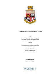
CHAPTER X.GEOMETRICAL MEANING OF DIFFERENTIATION.It is useful to consider what geometrical meaning can be given to thedifferential coefficient.In the first place, any function of x, such, for example, as x 2 , or √ x,or ax + b, can be plotted as a curve; and nowadays every schoolboy isfamiliar with the process of curve-plotting.YRPQdxdyyOxdxFig. 7.XLet P QR, in Fig. 7, be a portion of a curve plotted with respectto the axes of coordinates OX and OY . Consider any point Q on thiscurve, where the abscissa of the point is x and its ordinate is y. Nowobserve how y changes when x is varied. If x is made to increase by

CALCULUS MADE EASY 76a small increment dx, to the right, it will be observed that y also (inthis particular curve) increases by a small increment dy (because thisparticular curve happens to be an ascending curve). Then the ratio ofdy to dx is a measure of the degree to which the curve is sloping upbetween the two points Q and T . As a matter of fact, it can be seen onthe figure that the curve between Q and T has many different slopes,so that we cannot very well speak of the slope of the curve betweenQ and T . If, however, Q and T are so near each other that the smallportion QT of the curve is practically straight, then it is true to say thatthe ratio dy is the slope of the curve along QT . The straight line QTdxproduced on either side touches the curve along the portion QT only,and if this portion is indefinitely small, the straight line will touch thecurve at practically one point only, and be therefore a tangent to thecurve.This tangent to the curve has evidently the same slope as QT , sothat dy is the slope of the tangent to the curve at the point Q for whichdxthe value of dy is found.dxWe have seen that the short expression “the slope of a curve” hasno precise meaning, because a curve has so many slopes—in fact, everysmall portion of a curve has a different slope. “The slope of a curve ata point” is, however, a perfectly defined thing; it is the slope of a verysmall portion of the curve situated just at that point; and we have seenthat this is the same as “the slope of the tangent to the curve at thatpoint.”Observe that dx is a short step to the right, and dy the correspondingshort step upwards. These steps must be considered as short as

MEANING OF DIFFERENTIATION 77possible—in fact indefinitely short,—though in diagrams we have torepresent them by bits that are not infinitesimally small, otherwisethey could not be seen.dydxWe shall hereafter make considerable use of this circumstance thatrepresents the slope of the curve at any point.YdxdyOFig. 8.XIf a curve is sloping up at 45 ◦ at a particular point, as in Fig. 8, dyand dx will be equal, and the value of dydx = 1.If the curve slopes up steeper than 45 ◦ (Fig. 9), dy will be greaterdxthan 1.If the curve slopes up very gently, as in Fig. 10, dy will be a fractiondxsmaller than 1.For a horizontal line, or a horizontal place in a curve, dy = 0, andtherefore dydx = 0.If a curve slopes downward, as in Fig. 11, dy will be a step down,and must therefore be reckoned of negative value; hence dy will havedxnegative sign also.

CALCULUS MADE EASY 78YYdydxdydxOXOXFig. 9.Fig. 10.If the “curve” happens to be a straight line, like that in Fig. 12, thevalue of dy will be the same at all points along it. In other words itsdxslope is constant.If a curve is one that turns more upwards as it goes along to theright, the values of dy will become greater and greater with the increasingsteepness, as in Fig.dx13.If a curve is one that gets flatter and flatter as it goes along, thedyvalues of will become smaller and smaller as the flatter part isdxYQdxdyyOxdxFig. 11.X

MEANING OF DIFFERENTIATION 79YdxdydxdydxdyOXFig. 12.YdydxOdxdydxdyXFig. 13.reached, as in Fig. 14.If a curve first descends, and then goes up again, as in Fig. 15,presenting a concavity upwards, then clearly dy will first be negative,dxwith diminishing values as the curve flattens, then will be zero at thepoint where the bottom of the trough of the curve is reached; and fromthis point onward dy will have positive values that go on increasing. Indxsuch a case y is said to pass by a minimum. The minimum value of y isnot necessarily the smallest value of y, it is that value of y correspondingto the bottom of the trough; for instance, in Fig. 28 (p. 99), the valueof y corresponding to the bottom of the trough is 1, while y takes

CALCULUS MADE EASY 80YYy min.OXOXFig. 14.Fig. 15.elsewhere values which are smaller than this. The characteristic of aminimum is that y must increase on either side of it.N.B.—For the particular value of x that makes y a minimum, thevalue of dydx = 0.If a curve first ascends and then descends, the values of dy will bedxpositive at first; then zero, as the summit is reached; then negative,as the curve slopes downwards, as in Fig. 16. In this case y is said topass by a maximum, but the maximum value of y is not necessarily thegreatest value of y. In Fig. 28, the maximum of y is 2 1 , but this is3by no means the greatest value y can have at some other point of thecurve.N.B.—For the particular value of x that makes y a maximum, thevalue of dydx = 0.If a curve has the peculiar form of Fig. 17, the values of dydx willalways be positive; but there will be one particular place where theslope is least steep, where the value of dy will be a minimum; that is,dxless than it is at any other part of the curve.

MEANING OF DIFFERENTIATION 81YYy max.OXOXFig. 16.Fig. 17.If a curve has the form of Fig. 18, the value of dy will be negativedxin the upper part, and positive in the lower part; while at the nose ofthe curve where it becomes actually perpendicular, the value of dydx willbe infinitely great.YdxdyQOdxdyFig. 18.XNow that we understand that dy measures the steepness of a curvedxat any point, let us turn to some of the equations which we have alreadylearned how to differentiate.

CALCULUS MADE EASY 82(1) As the simplest case take this:y = x + b.It is plotted out in Fig. 19, using equal scales for x and y. If we putx = 0, then the corresponding ordinate will be y = b; that is to say, the“curve” crosses the y-axis at the height b. From here it ascends at 45 ◦ ;YYdybdxbOXOXFig. 19.Fig. 20.for whatever values we give to x to the right, we have an equal y toascend. The line has a gradient of 1 in 1.Now differentiate y = x + b, by the rules we have already learned(pp. 21 and 25 ante), and we get dydx = 1.The slope of the line is such that for every little step dx to the right,we go an equal little step dy upward. And this slope is constant—alwaysthe same slope.(2) Take another case:y = ax + b.

MEANING OF DIFFERENTIATION 83We know that this curve, like the preceding one, will start from aheight b on the y-axis. But before we draw the curve, let us find itsslope by differentiating; which gives dy = a. The slope will be constant,dxat an angle, the tangent of which is here called a. Let us assign to asome numerical value—say 1 . Then we must give it such a slope that3it ascends 1 in 3; or dx will be 3 times as great as dy; as magnified inFig. 21. So, draw the line in Fig. 20 at this slope.Fig. 21.origin.(3) Now for a slightly harder case.Let y = ax 2 + b.Again the curve will start on the y-axis at a height b above theNow differentiate. [If you have forgotten, turn back to p. 25; or,rather, don’t turn back, but think out the differentiation.]dydx = 2ax.This shows that the steepness will not be constant: it increases asx increases. At the starting point P , where x = 0, the curve (Fig. 22)has no steepness—that is, it is level. On the left of the origin, where xhas negative values, dy will also have negative values, or will descenddxfrom left to right, as in the Figure.

CALCULUS MADE EASY 84YRPQbOFig. 22.XLet us illustrate this by working out a particular instance. Takingthe equationand differentiating it, we gety = 1 4 x2 + 3,dydx = 1 2 x.Now assign a few successive values, say from 0 to 5, to x; and calculatethe corresponding values of y by the first equation; and of dy from thedxsecond equation. Tabulating results, we have:x 0 1 2 3 4 5y 3 3 1 44 5 1 47 9 1 4dydx0121 1 1 22 2 1 2Then plot them out in two curves, Figs. 23 and 24, in Fig. 23 plottingthe values of y against those of x and in Fig. 24 those of dydx againstthose of x. For any assigned value of x, the height of the ordinate inthe second curve is proportional to the slope of the first curve.

MEANING OF DIFFERENTIATION 8598765yy = 1 4 x2 + 3−3 −2 −1 0 1 2 3 4 514 x2bx−3 −2 −1dydx543210dydx = 1 2 x1 2 3 4 5xFig. 23.Fig. 24.If a curve comes to a sudden cusp, as in Fig. 25, the slope at thatpoint suddenly changes from a slope upward to a slope downward. InYOFig. 25.Xthat case dy will clearly undergo an abrupt change from a positive todxa negative value.The following examples show further applications of the principlesjust explained.

CALCULUS MADE EASY 86(4) Find the slope of the tangent to the curvey = 12x + 3,at the point where x = −1. Find the angle which this tangent makeswith the curve y = 2x 2 + 2.The slope of the tangent is the slope of the curve at the point wherethey touch one another (see p. 76); that is, it is the dy of the curve fordxthat point. Here dydx = − 1dyand for x = −1,2x2 dx = −1 , which is the2slope of the tangent and of the curve at that point. The tangent, beinga straight line, has for equation y = ax + b, and its slope is dydx = a,hence a = − 1 2 . Also if x = −1, y = 12(−1) + 3 = 2 1 ; and as the2tangent passes by this point, the coordinates of the point must satisfythe equation of the tangent, namelyy = − 1 2 x + b,so that 2 1 = −1 × (−1) + b and b = 2; the equation of the tangent is22therefore y = − 1 2 x + 2.Now, when two curves meet, the intersection being a point commonto both curves, its coordinates must satisfy the equation of eachone of the two curves; that is, it must be a solution of the system ofsimultaneous equations formed by coupling together the equations ofthe curves. Here the curves meet one another at points given by thesolution of⎧⎨ y = 2x 2 + 2,⎩ y = − 1x + 2 or 2 2x2 + 2 = − 1x + 2; 2

MEANING OF DIFFERENTIATION 87that is, x(2x + 1 2 ) = 0.This equation has for its solutions x = 0 and x = − 1 . The slope of4the curve y = 2x 2 + 2 at any point isdydx = 4x.For the point where x = 0, this slope is zero; the curve is horizontal.For the point wherex = − 1 4 ,dydx = −1;hence the curve at that point slopes downwards to the right at suchan angle θ with the horizontal that tan θ = 1; that is, at 45 ◦ to thehorizontal.The slope of the straight line is − 1 ; that is, it slopes downwards to2the right and makes with the horizontal an angle φ such that tan φ = 1;2that is, an angle of 26 ◦ 34 ′ . It follows that at the first point the curvecuts the straight line at an angle of 26 ◦ 34 ′ , while at the second it cutsit at an angle of 45 ◦ − 26 ◦ 34 ′ = 18 ◦ 26 ′ .(5) A straight line is to be drawn, through a point whose coordinatesare x = 2, y = −1, as tangent to the curve y = x 2 − 5x + 6. Find thecoordinates of the point of contact.The slope of the tangent must be the same as the dydxthat is, 2x − 5.of the curve;The equation of the straight line is y = ax+b, and as it is satisfied forthe values x = 2, y = −1, then −1 = a×2+b; also, its dydx = a = 2x−5.The x and the y of the point of contact must also satisfy both theequation of the tangent and the equation of the curve.

CALCULUS MADE EASY 88We have then⎧⎪⎨y = x 2 − 5x + 6,y = ax + b,(i)(ii)−1 = 2a + b,⎪⎩a = 2x − 5,(iii)(iv)four equations in a, b, x, y.Equations (i) and (ii) give x 2 − 5x + 6 = ax + b.Replacing a and b by their value in this, we getx 2 − 5x + 6 = (2x − 5)x − 1 − 2(2x − 5),which simplifies to x 2 − 4x + 3 = 0, the solutions of which are: x = 3and x = 1. Replacing in (i), we get y = 0 and y = 2 respectively; thetwo points of contact are then x = 1, y = 2, and x = 3, y = 0.Note.—In all exercises dealing with curves, students will find it extremelyinstructive to verify the deductions obtained by actually plottingthe curves.Exercises VIII.(See page 256 for Answers.)(1) Plot the curve y = 3 4 x2 −5, using a scale of millimetres. Measureat points corresponding to different values of x, the angle of its slope.Find, by differentiating the equation, the expression for slope; andsee, from a Table of Natural Tangents, whether this agrees with themeasured angle.

MEANING OF DIFFERENTIATION 89(2) Find what will be the slope of the curvey = 0.12x 3 − 2,at the particular point that has as abscissa x = 2.(3) If y = (x − a)(x − b), show that at the particular point of thecurve where dydx = 0, x will have the value 1 (a + b).2(4) Find the dydx of the equation y = x3 + 3x; and calculate thenumerical values of dydx for the points corresponding to x = 0, x = 1,2x = 1, x = 2.(5) In the curve to which the equation is x 2 +y 2 = 4, find the valuesof x at those points where the slope = 1.x 2(6) Find the slope, at any point, of the curve whose equation is3 + y2= 1; and give the numerical value of the slope at the place2 22 where x = 0, and at that where x = 1.(7) The equation of a tangent to the curve y = 5 − 2x + 0.5x 3 , beingof the form y = mx + n, where m and n are constants, find the valueof m and n if the point where the tangent touches the curve has x = 2for abscissa.(8) At what angle do the two curvescut one another?y = 3.5x 2 + 2 and y = x 2 − 5x + 9.5(9) Tangents to the curve y = ± √ 25 − x 2 are drawn at points forwhich x = 3 and x = 4. Find the coordinates of the point of intersectionof the tangents and their mutual inclination.

CALCULUS MADE EASY 90(10) A straight line y = 2x − b touches a curve y = 3x 2 + 2 at onepoint. What are the coordinates of the point of contact, and what isthe value of b?

CHAPTER XI.MAXIMA AND MINIMA.One of the principal uses of the process of differentiating is to find outunder what conditions the value of the thing differentiated becomes amaximum, or a minimum. This is often exceedingly important in engineeringquestions, where it is most desirable to know what conditionswill make the cost of working a minimum, or will make the efficiency amaximum.Now, to begin with a concrete case, let us take the equationy = x 2 − 4x + 7.By assigning a number of successive values to x, and finding the correspondingvalues of y, we can readily see that the equation representsa curve with a minimum.x 0 1 2 3 4 5y 7 4 3 4 7 12These values are plotted in Fig. 26, which shows that y has apparentlya minimum value of 3, when x is made equal to 2. But are yousure that the minimum occurs at 2, and not at 2 1 or at 1 3?4 4

CALCULUS MADE EASY 92Y7654321O1 2 3 4Fig. 26.XOf course it would be possible with any algebraic expression to workout a lot of values, and in this way arrive gradually at the particularvalue that may be a maximum or a minimum.Y4321−1 O 1−12 3 4 X−2−3−4Fig. 27.Here is another example:Let y = 3x − x 2 .

MAXIMA AND MINIMA 93Calculate a few values thus:x −1 0 1 2 3 4 5y −4 0 2 2 0 −4 −10Plot these values as in Fig. 27.It will be evident that there will be a maximum somewhere betweenx = 1 and x = 2; and the thing looks as if the maximum value of y oughtto be about 2 1. Try some intermediate values. If x = 1 1 , y = 2.187; if4 4x = 1 1 , y = 2.25; if x = 1.6, y = 2.24. How can we be sure that 2.25 is2the real maximum, or that it occurs exactly when x = 1 1?2Now it may sound like juggling to be assured that there is a wayby which one can arrive straight at a maximum (or minimum) valuewithout making a lot of preliminary trials or guesses. And that waydepends on differentiating. Look back to an earlier page (78) for theremarks about Figs. 14 and 15, and you will see that whenever a curvegets either to its maximum or to its minimum height, at that point itsdy= 0. Now this gives us the clue to the dodge that is wanted. Whendxthere is put before you an equation, and you want to find that valueof x that will make its y a minimum (or a maximum), first differentiateit, and having done so, write its dy as equal to zero, and then solvedxfor x. Put this particular value of x into the original equation, and youwill then get the required value of y. This process is commonly called“equating to zero.”To see how simply it works, take the example with which this chapteropens, namelyy = x 2 − 4x + 7.

CALCULUS MADE EASY 94Differentiating, we get:dydxNow equate this to zero, thus:= 2x − 4.2x − 4 = 0.Solving this equation for x, we get:2x = 4,x = 2.Now, we know that the maximum (or minimum) will occur exactlywhen x = 2.Putting the value x = 2 into the original equation, we gety = 2 2 − (4 × 2) + 7= 4 − 8 + 7= 3.Now look back at Fig. 26, and you will see that the minimum occurswhen x = 2, and that this minimum of y = 3.Try the second example (Fig. 24), which isDifferentiating,Equating to zero,y = 3x − x 2 .dydx = 3 − 2x.3 − 2x = 0,whence x = 1 1 2 ;

MAXIMA AND MINIMA 95and putting this value of x into the original equation, we find:y = 4 1 2 − (1 1 2 × 1 1 2 ),y = 2 1 4 .This gives us exactly the information as to which the method of tryinga lot of values left us uncertain.Now, before we go on to any further cases, we have two remarks tomake. When you are told to equate dy to zero, you feel at first (thatdxis if you have any wits of your own) a kind of resentment, because youknow that dy has all sorts of different values at different parts of thedxcurve, according to whether it is sloping up or down. So, when you aresuddenly told to writedydx = 0,you resent it, and feel inclined to say that it can’t be true. Now you willhave to understand the essential difference between “an equation,” and“an equation of condition.” Ordinarily you are dealing with equationsthat are true in themselves, but, on occasions, of which the present areexamples, you have to write down equations that are not necessarilytrue, but are only true if certain conditions are to be fulfilled; and youwrite them down in order, by solving them, to find the conditions whichmake them true. Now we want to find the particular value that x haswhen the curve is neither sloping up nor sloping down, that is, at theparticular place where dydy= 0. So, writing = 0 does not mean thatdx dxit always is = 0; but you write it down as a condition in order to seehow much x will come out if dy is to be zero.dx

CALCULUS MADE EASY 96The second remark is one which (if you have any wits of your own)you will probably have already made: namely, that this much-belaudedprocess of equating to zero entirely fails to tell you whether the x thatyou thereby find is going to give you a maximum value of y or a minimumvalue of y. Quite so. It does not of itself discriminate; it findsfor you the right value of x but leaves you to find out for yourselveswhether the corresponding y is a maximum or a minimum. Of course,if you have plotted the curve, you know already which it will be.For instance, take the equation:y = 4x + 1 x .Without stopping to think what curve it corresponds to, differentiateit, and equate to zero:whence x = 1 2 ;dydx = 4 − x−2 = 4 − 1 x 2 = 0;and, inserting this value,y = 4will be either a maximum or else a minimum. But which? You willhereafter be told a way, depending upon a second differentiation, (seeChap. XII., p. 109). But at present it is enough if you will simplytry any other value of x differing a little from the one found, and seewhether with this altered value the corresponding value of y is less orgreater than that already found.

MAXIMA AND MINIMA 97Try another simple problem in maxima and minima. Suppose youwere asked to divide any number into two parts, such that the productwas a maximum? How would you set about it if you did not know thetrick of equating to zero? I suppose you could worry it out by the ruleof try, try, try again. Let 60 be the number. You can try cutting it intotwo parts, and multiplying them together. Thus, 50 times 10 is 500; 52times 8 is 416; 40 times 20 is 800; 45 times 15 is 675; 30 times 30 is 900.This looks like a maximum: try varying it. 31 times 29 is 899, which isnot so good; and 32 times 28 is 896, which is worse. So it seems thatthe biggest product will be got by dividing into two equal halves.Now see what the calculus tells you. Let the number to be cut intotwo parts be called n. Then if x is one part, the other will be n − x,and the product will be x(n − x) or nx − x 2 . So we write y = nx − x 2 .Now differentiate and equate to zero;Solving for x, we getdydx = n − 2x = 0n2 = x.So now we know that whatever number n may be, we must divide itinto two equal parts if the product of the parts is to be a maximum;and the value of that maximum product will always be = 1 4 n2 .This is a very useful rule, and applies to any number of factors, sothat if m + n + p = a constant number, m × n × p is a maximum whenm = n = p.

CALCULUS MADE EASY 98Test Case.Let us at once apply our knowledge to a case that we can test.Let y = x 2 − x;and let us find whether this function has a maximum or minimum; andif so, test whether it is a maximum or a minimum.Differentiating, we getEquating to zero, we getdydx2x − 1 = 0,whence 2x = 1,or x = 1 2 .= 2x − 1.That is to say, when x is made = 1 , the corresponding value of y2will be either a maximum or a minimum. Accordingly, putting x = 1 2in the original equation, we gety = ( 1 2 )2 − 1 2 ,or y = − 1 4 .Is this a maximum or a minimum? To test it, try putting x a littlebigger than 1 ,—say make x = 0.6. Then2y = (0.6) 2 − 0.6 = 0.36 − 0.6 = −0.24,which is higher up than −0.25; showing that y = −0.25 is a minimum.Plot the curve for yourself, and verify the calculation.

MAXIMA AND MINIMA 99Further Examples.A most interesting example is afforded by a curve that has both amaximum and a minimum. Its equation is:Nowy = 1 3 x3 − 2x 2 + 3x + 1.dydx = x2 − 4x + 3.−1Y654321O 1−12 3 4 5−2−3−4XFig. 28.Equating to zero, we get the quadratic,x 2 − 4x + 3 = 0;and solving the quadratic gives us two roots, viz.⎧⎨ x = 3⎩ x = 1.

CALCULUS MADE EASY 100Now, when x = 3, y = 1; and when x = 1, y = 2 1 . The first of3these is a minimum, the second a maximum.The curve itself may be plotted (as in Fig. 28) from the valuescalculated, as below, from the original equation.x −1 0 1 2 3 4 5 6y −4 1 31 2 1 31 2 31 2 1 37 2 319A further exercise in maxima and minima is afforded by the followingexample:The equation to a circle of radius r, having its centre C at the pointwhose coordinates are x = a, y = b, as depicted in Fig. 29, is:(y − b) 2 + (x − a) 2 = r 2 .YrbxCyOaFig. 29.XThis may be transformed intoy = √ r 2 − (x − a) 2 + b.

MAXIMA AND MINIMA 101Now we know beforehand, by mere inspection of the figure, thatwhen x = a, y will be either at its maximum value, b + r, or else at itsminimum value, b −r. But let us not take advantage of this knowledge;let us set about finding what value of x will make y a maximum or aminimum, by the process of differentiating and equating to zero.which reduces todydx = 1 1√ × (2a − 2x),2 r2 − (x − a)2dydx =a − x√r2 − (x − a) 2 .Then the condition for y being maximum or minimum is:a − x√r2 − (x − a) 2 = 0.Since no value whatever of x will make the denominator infinite,the only condition to give zero isx = a.Inserting this value in the original equation for the circle, we findy = √ r 2 + b;and as the root of r 2 is either +r or −r, we have two resulting valuesof y,⎧⎨ y = b + r⎩ y = b − r.

CALCULUS MADE EASY 102The first of these is the maximum, at the top; the second the minimum,at the bottom.If the curve is such that there is no place that is a maximum orminimum, the process of equating to zero will yield an impossible result.For instance:Let y = ax 3 + bx + c.Thendydx = 3ax2 + b.Equating this to zero, we get 3ax 2 + b = 0,x 2 = −b√−b3a , and x = , which is impossible.3aTherefore y has no maximum nor minimum.A few more worked examples will enable you to thoroughly masterthis most interesting and useful application of the calculus.(1) What are the sides of the rectangle of maximum area inscribedin a circle of radius R?If one side be called x,the other side = √ (diagonal) 2 − x 2 ;and as the diagonal of the rectangle is necessarily a diameter, the otherside = √ 4R 2 − x 2 .Then, area of rectangle S = x √ 4R 2 − x 2 ,dSdx = x × d (√ 4R 2 − x ) 2 + √ 4Rdx2 − x 2 × d(x)dx .If you have forgotten how to differentiate √ 4R 2 − x 2 , here is a hint:write 4R 2 − x 2 = w and y = √ w, and seek dy dwand ; fight it out,dw dxand only if you can’t get on refer to page 66.

MAXIMA AND MINIMA 103You will getdSdx = x × − x√4R2 − x + √ 4R 2 − x 2 = 4R2 − 2x 2√ 2 4R2 − x . 2For maximum or minimum we must have4R 2 − 2x 2√4R2 − x 2 = 0;that is, 4R 2 − 2x 2 = 0 and x = R √ 2.The other side = √ 4R 2 − 2R 2 = R √ 2; the two sides are equal; thefigure is a square the side of which is equal to the diagonal of the squareconstructed on the radius. In this case it is, of course, a maximum withwhich we are dealing.(2) What is the radius of the opening of a conical vessel the slopingside of which has a length l when the capacity of the vessel is greatest?If R be the radius and H the corresponding height, H = √ l 2 − R 2 .Volume V = πR 2 × H √3 = l2 − R πR2 ×2.3Proceeding as in the previous problem, we getfor maximum or minimum.dVdR = RπR2 × −3 √ l 2 − R + 2πR √l2 − R 2 32= 2πR(l2 − R 2 ) − πR 33 √ = 0l 2 − R 2Or, 2πR(l 2 − R 2 ) − πR 2obviously.√= 0, and R = l(3) Find the maxima and minima of the functiony =x4 − x + 4 − xx .23, for a maximum,

CALCULUS MADE EASY 104We getdydxfor maximum or minimum; or(4 − x) − (−x) −x − (4 − x)= + = 0(4 − x) 2 x 24(4 − x) − 4 = 0 and x = 2.2 x2 There is only one value, hence only one maximum or minimum.For x = 2, y = 2,for x = 1.5, y = 2.27,for x = 2.5, y = 2.27;it is therefore a minimum. (It is instructive to plot the graph of thefunction.)(4) Find the maxima and minima of the function y = √ 1 + x +√ 1 − x. (It will be found instructive to plot the graph.)Differentiating gives at once (see example No. 1, p. 67)for maximum or minimum.dydx = 12 √ 1 + x − 12 √ 1 − x = 0Hence √ 1 + x = √ 1 − x and x = 0, the only solutionFor x = 0, y = 2.For x = ±0.5, y = 1.932, so this is a maximum.(5) Find the maxima and minima of the functiony = x2 − 52x − 4 .

MAXIMA AND MINIMA 105We havefor maximum or minimum; ordydx = (2x − 4) × 2x − (x2 − 5)2= 0(2x − 4) 22x 2 − 8x + 10(2x − 4) 2 = 0;or x 2 − 4x + 5 = 0; which has for solutionsx = 5 2 ± √ −1.These being imaginary, there is no real value of x for which dydx = 0;hence there is neither maximum nor minimum.(6) Find the maxima and minima of the function(y − x 2 ) 2 = x 5 .This may be written y = x 2 ± x 5 2 .dydx = 2x ± 5 2 x 3 2 = 0for maximum or minimum;that is, x(2± 5 2 x 1 2 ) = 0, which is satisfied for x = 0, and for 2± 5 2 x 1 2 = 0,that is for x = 16 . So there are two solutions.25Taking first x = 0. If x = −0.5, y = 0.25 ± 2√ −(.5) 5 , and ifx = +0.5, y = 0.25 ± 2√ (.5) 5 . On one side y is imaginary; that is,there is no value of y that can be represented by a graph; the latter istherefore entirely on the right side of the axis of y (see Fig. 30).On plotting the graph it will be found that the curve goes to theorigin, as if there were a minimum there; but instead of continuingbeyond, as it should do for a minimum, it retraces its steps (forming

CALCULUS MADE EASY 106what is called a “cusp”). There is no minimum, therefore, although thecondition for a minimum is satisfied, namely dy = 0. It is necessarydxtherefore always to check by taking one value on either side.y0.30.20.10 0.2 0.4 0.6 0.8 1.0Fig. 30.xNow, if we take x = 16 = 0.64. If x = 0.64, y = 0.7373 and25y = 0.0819; if x = 0.6, y becomes 0.6389 and 0.0811; and if x = 0.7,y becomes 0.8996 and 0.0804.This shows that there are two branches of the curve; the upper onedoes not pass through a maximum, but the lower one does.(7) A cylinder whose height is twice the radius of the base is increasingin volume, so that all its parts keep always in the same proportionto each other; that is, at any instant, the cylinder is similar to theoriginal cylinder. When the radius of the base is r feet, the surfacearea is increasing at the rate of 20 square inches per second; at what

MAXIMA AND MINIMA 107rate is its volume then increasing?Area = S = 2(πr 2 ) + 2πr × 2r = 6πr 2 .Volume = V = πr 2 × 2r = 2πr 3 .dSdr = 12πr,dVdr = 6πr2 ,dS = 12πr dr = 20, dr = 2012πr ,dV = 6πr 2 dr = 6πr 2 × 2012πr = 10r.The volume changes at the rate of 10r cubic inches.Make other examples for yourself.offer such a wealth for interesting examples.There are few subjects whichExercises IX.(See page 257 for Answers.)(1) What values of x will make y a maximum and a minimum, ify =x2x + 1 ?(2) What value of x will make y a maximum in the equation y =xa 2 + x ? 2(3) A line of length p is to be cut up into 4 parts and put togetheras a rectangle. Show that the area of the rectangle will be a maximumif each of its sides is equal to 1 4 p.(4) A piece of string 30 inches long has its two ends joined togetherand is stretched by 3 pegs so as to form a triangle. What is the largesttriangular area that can be enclosed by the string?

CALCULUS MADE EASY 108(5) Plot the curve corresponding to the equationy = 10x + 108 − x ;also find dy , and deduce the value of x that will make y a minimum;dxand find that minimum value of y.(6) If y = x 5 − 5x, find what values of x will make y a maximum ora minimum.(7) What is the smallest square that can be inscribed in a givensquare?(8) Inscribe in a given cone, the height of which is equal to the radiusof the base, a cylinder (a) whose volume is a maximum; (b) whoselateral area is a maximum; (c) whose total area is a maximum.(9) Inscribe in a sphere, a cylinder (a) whose volume is a maximum;(b) whose lateral area is a maximum; (c) whose total area is amaximum.(10) A spherical balloon is increasing in volume. If, when its radiusis r feet, its volume is increasing at the rate of 4 cubic feet per second,at what rate is its surface then increasing?(11) Inscribe in a given sphere a cone whose volume is a maximum.(12) The current C given by a battery of N similar voltaic cells isC =n × E , where E, R, r, are constants and n is the number ofR + rn2Ncells coupled in series. Find the proportion of n to N for which thecurrent is greatest.

CHAPTER XII.CURVATURE OF CURVES.Returning to the process of successive differentiation, it may beasked: Why does anybody want to differentiate twice over? We knowthat when the variable quantities are space and time, by differentiatingtwice over we get the acceleration of a moving body, and that in thegeometrical interpretation, as applied to curves, dy means the slope ofdxthe curve. But what can d2 ymean in this case? Clearly it means thedx2 rate (per unit of length x) at which the slope is changing—in brief, itis a measure of the curvature of the slope.YYOXOXFig. 31.Fig. 32.Suppose a slope constant, as in Fig. 31.

CALCULUS MADE EASY 110Here, dy is of constant value.dxSuppose, however, a case in ( which, ) like Fig. 32, the slope itself isdyddxgetting greater upwards, then , that is, d2 y, will be positive.dxdx2 If the slope is becoming less as you go to the right (as in Fig. 14,p. 80), or as in Fig. 33, then, even though the curve may be goingupward, since the change is such as to diminish its slope, its d2 ydx will 2be negative.YOFig. 33.XIt is now time to initiate you into another secret—how to tellwhether the result that you get by “equating to zero” is a maximum ora minimum. The trick is this: After you have differentiated (so as toget the expression which you equate to zero), you then differentiate asecond time, and look whether the result of the second differentiationis positive or negative. If d2 ycomes out positive, then you know thatdx2 the value of y which you got was a minimum; but if d2 ycomes outdx 2negative, then the value of y which you got must be a maximum. That’s

CURVATURE OF CURVES 111the rule.The reason of it ought to be quite evident. Think of any curve thathas a minimum point in it (like Fig. 15, p. 80), or like Fig. 34, where thepoint of minimum y is marked M, and the curve is concave upwards.To the left of M the slope is downward, that is, negative, and is gettingless negative. To the right of M the slope has become upward, andis getting more and more upward. Clearly the change of slope as theYYMMy max.y min.OxFig. 34.XOxFig. 35.Xcurve passes through M is such that d2 yis positive, for its operation,dx2 as x increases toward the right, is to convert a downward slope into anupward one.Similarly, consider any curve that has a maximum point in it (likeFig. 16, p. 81), or like Fig. 35, where the curve is convex, and the maximumpoint is marked M. In this case, as the curve passes through Mfrom left to right, its upward slope is converted into a downward ornegative slope, so that in this case the “slope of the slope” d2 ydx is 2negative.Go back now to the examples of the last chapter and verify in this

CALCULUS MADE EASY 112way the conclusions arrived at as to whether in any particular casethere is a maximum or a minimum. You will find below a few workedout examples.(1) Find the maximum or minimum of(a) y = 4x 2 − 9x − 6; (b) y = 6 + 9x − 4x 2 ;and ascertain if it be a maximum or a minimum in each case.(a)(b)dydx = 8x − 9 = 0; x = 1 1 , and y = −11.065.8d 2 ydx = 8; it is +; hence it is a minimum.2dydx = 9 − 8x = 0; x = 1 1 ; and y = +11.065.8d 2 ydx = −8; it is −; hence it is a maximum.2(2) Find the maxima and minima of the function y = x 3 − 3x + 16.dydx = 3x2 − 3 = 0; x 2 = 1; and x = ±1.d 2 y= 6x; for x = 1; it is +;dx2 hence x = 1 corresponds to a minimum y = 14. For x = −1 it is −;hence x = −1 corresponds to a maximum y = +18.(3) Find the maxima and minima of y = x − 1x 2 + 2 .dydx = (x2 + 2) × 1 − (x − 1) × 2x(x 2 + 2) 2 = 2x − x2 + 2(x 2 + 2) 2 = 0;

CURVATURE OF CURVES 113or x 2 − 2x − 2 = 0, whose solutions are x = +2.73 and x = −0.73.d 2 ydx = + 2) 2 × (2x − 2) − (x 2 − 2x − 2)(4x 3 + 8x)2 −(x2 (x 2 + 2) 4= − 2x5 − 6x 4 − 8x 3 − 8x 2 − 24x + 8(x 2 + 2) 4 .The denominator is always positive, so it is sufficient to ascertainthe sign of the numerator.0.183.If we put x = 2.73, the numerator is negative; the maximum, y =If we put x = −0.73, the numerator is positive; the minimum,y = −0.683.(4) The expense C of handling the products of a certain factoryvaries with the weekly output P according to the relation C = aP +b+ d, where a, b, c, d are positive constants. For what output willc + Pthe expense be least?hence a =dCdP = a − b= 0 for maximum or minimum;(c + P )2b(c + P ) 2 and P = ± √ba − c.As the output cannot be negative, P = +√ba − c.Nowd 2 C + 2P )= +b(2cdP2(c + P ) , 4bwhich is positive for all the values of P ; hence P = +√−c correspondsato a minimum.

CALCULUS MADE EASY 114(5) The total cost per hour C of lighting a building with N lampsof a certain kind isC = N(Clt + EP C )e,1000where E is the commercial efficiency (watts per candle),P is the candle power of each lamp,t is the average life of each lamp in hours,C l = cost of renewal in pence per hour of use,C e = cost of energy per 1000 watts per hour.Moreover, the relation connecting the average life of a lamp withthe commercial efficiency at which it is run is approximately t = mE n ,where m and n are constants depending on the kind of lamp.Find the commercial efficiency for which the total cost of lightingwill be least.We havefor maximum or minimum.(ClC = Nm E−n + P C )e1000 E ,dCdE = P C e1000 − nC lm E−(n+1) = 0E n+1 = 1000 × nC lmP C eand E = n+1 √1000 × nClmP C e.This is clearly for minimum, sinced 2 CdE 2 = (n + 1)nC lm E−(n+2) ,

CURVATURE OF CURVES 115which is positive for a positive value of E.For a particular type of 16 candle-power lamps, C l = 17 pence,C e = 5 pence; and it was found that m = 10 and n = 3.6.E = 4.6 √1000 × 3.6 × 1710 × 16 × 5= 2.6 watts per candle-power.Exercises X.(You are advised to plot the graph of any numericalexample.) (See p. 258 for the Answers.)(1) Find the maxima and minima ofy = x 3 + x 2 − 10x + 8.(2) Given y = b a x − cx2 , find expressions for dydx , and for d2 ydx , also 2find the value of x which makes y a maximum or a minimum, and showwhether it is maximum or minimum.(3) Find how many maxima and how many minima there are in thecurve, the equation to which isy = 1 − x22 + x424 ;and how many in that of which the equation isy = 1 − x22 + x424 − x6720 .(4) Find the maxima and minima ofy = 2x + 1 + 5 x 2 .

CALCULUS MADE EASY 116(5) Find the maxima and minima ofy =3x 2 + x + 1 .(6) Find the maxima and minima ofy =5x2 + x 2 .(7) Find the maxima and minima ofy =3xx 2 − 3 + x 2 + 5.(8) Divide a number N into two parts in such a way that three timesthe square of one part plus twice the square of the other part shall bea minimum.(9) The efficiency u of an electric generator at different values ofoutput x is expressed by the general equation:u =xa + bx + cx 2 ;where a is a constant depending chiefly on the energy losses in the ironand c a constant depending chiefly on the resistance of the copper parts.Find an expression for that value of the output at which the efficiencywill be a maximum.(10) Suppose it to be known that consumption of coal by a certainsteamer may be represented by the formula y = 0.3+0.001v 3 ; where y isthe number of tons of coal burned per hour and v is the speed expressedin nautical miles per hour. The cost of wages, interest on capital, anddepreciation of that ship are together equal, per hour, to the cost of

CURVATURE OF CURVES 1171 ton of coal. What speed will make the total cost of a voyage of 1000nautical miles a minimum? And, if coal costs 10 shillings per ton, whatwill that minimum cost of the voyage amount to?(11) Find the maxima and minima ofy = ± x √x(10 − x).6(12) Find the maxima and minima ofy = 4x 3 − x 2 − 2x + 1.

CHAPTER XIII.OTHER USEFUL DODGES.Partial Fractions.We have seen that when we differentiate a fraction we have to performa rather complicated operation; and, if the fraction is not itself a simpleone, the result is bound to be a complicated expression. If we couldsplit the fraction into two or more simpler fractions such that theirsum is equivalent to the original fraction, we could then proceed bydifferentiating each of these simpler expressions.And the result ofdifferentiating would be the sum of two (or more) differentials, each oneof which is relatively simple; while the final expression, though of courseit will be the same as that which could be obtained without resortingto this dodge, is thus obtained with much less effort and appears in asimplified form.Let us see how to reach this result.Try first the job of addingtwo fractions together to form a resultant fraction. Take, for example,1the two fractionsx + 1 and 2x − 1 . Every schoolboy can add thesetogether and find their sum to be 3x + 1 . And in the same way he canx 2 − 1add together three or more fractions. Now this process can certainlybe reversed: that is to say, that if this last expression were given, it

OTHER USEFUL DODGES 119is certain that it can somehow be split back again into its originalcomponents or partial fractions. Only we do not know in every casethat may be presented to us how we can so split it. In order to findthis out we shall consider a simple case at first. But it is importantto bear in mind that all which follows applies only to what are called“proper” algebraic fractions, meaning fractions like the above, whichhave the numerator of a lesser degree than the denominator; that is,those in which the highest index of x is less in the numerator than inthe denominator. If we have to deal with such an expression as x2 + 2x 2 − 1 ,we can simplify it by division, since it is equivalent to 1 + 3x 2 − 1 ; and3is a proper algebraic fraction to which the operation of splittingx 2 − 1into partial fractions can be applied, as explained hereafter.Case I.If we perform many additions of two or more fractionsthe denominators of which contain only terms in x, and no terms inx 2 , x 3 , or any other powers of x, we always find that the denominatorof the final resulting fraction is the product of the denominators ofthe fractions which were added to form the result. It follows that byfactorizing the denominator of this final fraction, we can find every oneof the denominators of the partial fractions of which we are in search.Suppose we wish to go back from 3x + 1 to the components whichx 2 − 11we know arex + 1 and 2. If we did not know what those componentswere we can still prepare the way byx − 1writing:3x + 1x 2 − 1 = 3x + 1(x + 1)(x − 1) = x + 1 + x − 1 ,leaving blank the places for the numerators until we know what to put

CALCULUS MADE EASY 120there. We always may assume the sign between the partial fractionsto be plus, since, if it be minus, we shall simply find the correspondingnumerator to be negative. Now, since the partial fractions are properfractions, the numerators are mere numbers without x at all, and wecan call them A, B, C . . . as we please. So, in this case, we have:3x + 1x 2 − 1 =Ax + 1 +Bx − 1 .If now we perform the addition of these two partial fractions, weA(x − 1) + B(x + 1)3x + 1get ; and this must be equal to(x + 1)(x − 1)(x + 1)(x − 1) .And, as the denominators in these two expressions are the same, thenumerators must be equal, giving us:3x + 1 = A(x − 1) + B(x + 1).Now, this is an equation with two unknown quantities, and it wouldseem that we need another equation before we can solve them and findA and B. But there is another way out of this difficulty. The equationmust be true for all values of x; therefore it must be true for such valuesof x as will cause x − 1 and x + 1 to become zero, that is for x = 1 andfor x = −1 respectively. If we make x = 1, we get 4 = (A×0)+(B ×2),so that B = 2; and if we make x = −1, we get −2 = (A×−2)+(B ×0),so that A = 1. Replacing the A and B of the partial fractions by these1new values, we find them to becomex + 1 and 2; and the thing isx − 1done.As a farther example, let us take the fraction 4x2 + 2x − 14x 3 + 3x 2 − x − 3 . Thedenominator becomes zero when x is given the value 1; hence x − 1 isa factor of it, and obviously then the other factor will be x 2 + 4x + 3;

OTHER USEFUL DODGES 121and this can again be decomposed into (x + 1)(x + 3). So we may writethe fraction thus:4x 2 + 2x − 14x 3 + 3x 2 − x − 3 =making three partial factors.Proceeding as before, we findAx + 1 +Bx − 1 +Cx + 3 ,4x 2 + 2x − 14 = A(x − 1)(x + 3) + B(x + 1)(x + 3) + C(x + 1)(x − 1).Now, if we make x = 1, we get:−8 = (A × 0) + B(2 × 4) + (C × 0); that is, B = −1.If x = −1, we get:−12 = A(−2 × 2) + (B × 0) + (C × 0); whence A = 3.If x = −3, we get:16 = (A × 0) + (B × 0) + C(−2 × −4); whence C = 2.So then the partial fractions are:3x + 1 − 1x − 1 + 2x + 3 ,which is far easier to differentiate with respect to x than the complicatedexpression from which it is derived.

CALCULUS MADE EASY 122Case II. If some of the factors of the denominator contain termsin x 2 , and are not conveniently put into factors, then the correspondingnumerator may contain a term in x, as well as a simple number; andhence it becomes necessary to represent this unknown numerator notby the symbol A but by Ax + B; the rest of the calculation being madeas before.−x 2 − 3Try, for instance:(x 2 + 1)(x + 1) .−x 2 − 3(x 2 + 1)(x + 1) = Ax + Bx 2 + 1 + Cx + 1 ;−x 2 − 3 = (Ax + B)(x + 1) + C(x 2 + 1).Putting x = −1, we get −4 = C × 2; and C = −2;hence −x 2 − 3 = (Ax + B)(x + 1) − 2x 2 − 2;and x 2 − 1 = Ax(x + 1) + B(x + 1).hencePutting x = 0, we get −1 = B;x 2 − 1 = Ax(x + 1) − x − 1; or x 2 + x = Ax(x + 1);and x + 1 = A(x + 1),so that A = 1, and the partial fractions are:x − 1x 2 + 1 − 2x + 1 .Take as another example the fractionx 3 − 2(x 2 + 1)(x 2 + 2) .

OTHER USEFUL DODGES 123We getx 3 − 2(x 2 + 1)(x 2 + 2) = Ax + Bx 2 + 1 + Cx + Dx 2 + 2= (Ax + B)(x2 + 2) + (Cx + D)(x 2 + 1).(x 2 + 1)(x 2 + 2)In this case the determination of A, B, C, D is not so easy.will be simpler to proceed as follows: Since the given fraction andthe fraction found by adding the partial fractions are equal, and haveidentical denominators, the numerators must also be identically thesame. In such a case, and for such algebraical expressions as those withwhich we are dealing here, the coefficients of the same powers of x areequal and of same sign.Hence, sincex 3 − 2 = (Ax + B)(x 2 + 2) + (Cx + D)(x 2 + 1)we have 1 = A + C;= (A + C)x 3 + (B + D)x 2 + (2A + C)x + 2B + D,0 = B + D (the coefficient of x 2 in the leftexpression being zero); 0 = 2A + C; and −2 = 2B + D.ItHere arefour equations, from which we readily obtain A = −1; B = −2; C = 2;2(x + 1)D = 0; so that the partial fractions arex 2 + 2 − x + 2 . This methodx 2 + 1can always be used; but the method shown first will be found thequickest in the case of factors in x only.Case III. When, among the factors of the denominator there aresome which are raised to some power, one must allow for the possibleexistence of partial fractions having for denominator the severalpowers of that factor up to the highest. For instance, in splitting the

CALCULUS MADE EASY 124fraction 3x2 − 2x + 1we must allow for the possible existence of a(x + 1) 2 (x − 2)denominator x + 1 as well as (x + 1) 2 and (x − 2).It maybe thought, however, that, since the numerator of the fractionthe denominator of which is (x + 1) 2 may contain terms in x, we mustallow for this in writing Ax + B for its numerator, so that3x 2 − 2x + 1(x + 1) 2 (x − 2) = Ax + B(x + 1) + C2 x + 1 + Dx − 2 .If, however, we try to find A, B, C and D in this case, we fail, becausewe get four unknowns; and we have only three relations connectingthem, yetwe getBut if we write3x 2 − 2x + 1(x + 1) 2 (x − 2) = x − 1(x + 1) + 12 x + 1 + 1x − 2 .3x 2 − 2x + 1(x + 1) 2 (x − 2) = A(x + 1) + B2 x + 1 + Cx − 2 ,3x 2 − 2x + 1 = A(x − 2) + B(x + 1)(x − 2) + C(x + 1) 2 ,which gives C = 1 for x = 2. Replacing C by its value, transposing,gathering like terms and dividing by x − 2, we get −2x = A + B(x + 1),which gives A = −2 for x = −1. Replacing A by its value, we get2x = −2 + B(x + 1).Hence B = 2; so that the partial fractions are:2x + 1 − 2(x + 1) 2 + 1x − 2 ,

OTHER USEFUL DODGES 1251instead ofx + 1 + x − 1(x + 1) + 1 stated above as being the fractions2 x − 2from which 3x2 − 2x + 1was obtained. The mystery is cleared if we(x + 1) 2 (x − 2)x − 1observe that(x + 1) can itself be split into the two fractions 12 x + 1 −2, so that the three fractions given are really equivalent to(x + 1)21x + 1 + 1x + 1 − 2(x + 1) + 12 x − 2 = 2x + 1 − 2(x + 1) + 12 x − 2 ,which are the partial fractions obtained.We see that it is sufficient to allow for one numerical term in eachnumerator, and that we always get the ultimate partial fractions.When there is a power of a factor of x 2 in the denominator, however,the corresponding numerators must be of the form Ax+B; for example,which gives3x − 1(2x 2 − 1) 2 (x + 1) = Ax + B(2x 2 − 1) + Cx + D2 2x 2 − 1 + Ex + 1 ,3x − 1 = (Ax + B)(x + 1) + (Cx + D)(x + 1)(2x 2 − 1) + E(2x 2 − 1) 2 .For x = −1, this gives E = −4. Replacing, transposing, collectinglike terms, and dividing by x + 1, we get16x 3 − 16x 2 + 3 = 2Cx 3 + 2Dx 2 + x(A − C) + (B − D).Hence 2C = 16 and C = 8; 2D = −16 and D = −8; A − C = 0 orA − 8 = 0 and A = 8, and finally, B − D = 3 or B = −5. So that weobtain as the partial fractions:(8x − 5) 8(x − 1)+(2x 2 − 1)22x 2 − 1 − 4x + 1 .

CALCULUS MADE EASY 126It is useful to check the results obtained. The simplest way is toreplace x by a single value, say +1, both in the given expression and inthe partial fractions obtained.Whenever the denominator contains but a power of a single factor,a very quick method is as follows:4x + 1Taking, for example, , let x + 1 = z; then x = z − 1.(x + 1)3Replacing, we get4(z − 1) + 1z 3 = 4z − 3z 3 = 4 z 2 − 3 z 3 .The partial fractions are, therefore,4(x + 1) − 32 (x + 1) . 3Application to differentiation.5 − 4xy =; we have6x 2 + 7x − 3Let it be required to differentiatedydx = + 7x − 3) × 4 + (5 − 4x)(12x + 7)−(6x2 (6x 2 + 7x − 3) 2= 24x2 − 60x − 23(6x 2 + 7x − 3) 2 .If we split the given expression intowe get, however,13x − 1 − 22x + 3 ,dydx = − 3(3x − 1) 2 + 4(2x + 3) 2 ,

OTHER USEFUL DODGES 127which is really the same result as above split into partial fractions.But the splitting, if done after differentiating, is more complicated, aswill easily be seen. When we shall deal with the integration of suchexpressions, we shall find the splitting into partial fractions a preciousauxiliary (see p. 228).Exercises XI.Split into fractions:(See page 259 for Answers.)(1)(3)(5)3x + 5(x − 3)(x + 4) . (2) 3x − 4(x − 1)(x − 2) .3x + 5x 2 + x − 12 . (4) x + 1x 2 − 7x + 12 .x − 8(2x + 3)(3x − 2) . (6)x 2 − 13x + 26(x − 2)(x − 3)(x − 4) .(7)(8)(9)(11)(13)x 2 − 3x + 1(x − 1)(x + 2)(x − 3) .5x 2 + 7x + 1(2x + 1)(3x − 2)(3x + 1) .x 2x 3 − 1 . (10) x4 + 1x 3 + 1 .5x 2 + 6x + 4(x + 1)(x 2 + x + 1) . (12)x(x 2 − 1)(x + 1) . (14)x(x − 1)(x − 2) 2 .x + 3(x + 2) 2 (x − 1) .

CALCULUS MADE EASY 128(15)3x 2 + 2x + 1(x + 2)(x 2 + x + 1) . (16) 5x2 + 8x − 12.2 (x + 4) 3(17) 7x2 + 9x − 1(3x − 2) 4 . (18)x 2(x 3 − 8)(x − 2) .Differential of an Inverse Function.Consider the function (see p. 13) y = 3x; it can be expressed in theform x = y ; this latter form is called the inverse function to the one3originally given.dyIf y = 3x,dx = 3; if x = y 3 ,dxdy = 1 , and we see that3dydx = 1dxdyordydx × dxdy = 1.Consider y = 4x 2 , dydxx = y 1 22= 8x; the inverse function is, anddxdy = 14 √ y = 14 × 2x = 18x .Here againdydx × dxdy = 1.It can be shown that for all functions which can be put into theinverse form, one can always writedydx × dxdy = 1 or dydx = 1dxdy.

OTHER USEFUL DODGES 129It follows that, being given a function, if it be easier to differentiatethe inverse function, this may be done, and the reciprocal of the differentialcoefficient of the inverse function gives the differential coefficientof the given function itself.As an example, suppose that we wish to differentiate y = 2 √3x − 1.We have seen one way of doing this, by writing u = 3 − 1, and findingxdy duand . This givesdu dxdydx = − 3√ .32x 2 x − 1If we had forgotten how to proceed by this method, or wished tocheck our result by some other way of obtaining the differential coefficient,or for any other reason we could not use the ordinary method,we can proceed as follows: The inverse function is x = 31 + y 2 .hencedydx = 1dxdydxdy = − 3 × 2y(1 + y 2 ) = − 6y2 (1 + y 2 ) ; 2= − (1 + y2 ) 26y= −Let us take as an other example y =(1 + 3 x − 1 ) 23√ = − √ .3 36 × 2 x − 1 2x 2 x − 113√θ + 5.The inverse function is θ = 1 y 3 − 5 or θ = y−3 − 5, anddθdy = −3y−4 = −3 3√ (θ + 5) 4 .

CALCULUS MADE EASY 130It follows that dydx = − 13 √ , as might have been found otherwise.(θ + 5)4We shall find this dodge most useful later on; meanwhile you areadvised to become familiar with it by verifying by its means the resultsobtained in Exercises I. (p. 24), Nos. 5, 6, 7; Examples (p. 67), Nos.1, 2, 4; and Exercises VI. (p. 72), Nos. 1, 2, 3 and 4.You will surely realize from this chapter and the preceding, that inmany respects the calculus is an art rather than a science: an art onlyto be acquired, as all other arts are, by practice. Hence you shouldwork many examples, and set yourself other examples, to see if you canwork them out, until the various artifices become familiar by use.

CHAPTER XIV.ON TRUE COMPOUND INTEREST AND THE LAWOF ORGANIC GROWTH.Let there be a quantity growing in such a way that the increment ofits growth, during a given time, shall always be proportional to its ownmagnitude. This resembles the process of reckoning interest on moneyat some fixed rate; for the bigger the capital, the bigger the amount ofinterest on it in a given time.Now we must distinguish clearly between two cases, in our calculation,according as the calculation is made by what the arithmetic bookscall “simple interest,” or by what they call “compound interest.” Forin the former case the capital remains fixed, while in the latter theinterest is added to the capital, which therefore increases by successiveadditions.(1) At simple interest. Consider a concrete case. Let the capital atstart be £100, and let the rate of interest be 10 per cent. per annum.Then the increment to the owner of the capital will be £10 every year.Let him go on drawing his interest every year, and hoard it by puttingit by in a stocking, or locking it up in his safe. Then, if he goes on for10 years, by the end of that time he will have received 10 increments

CALCULUS MADE EASY 132of £10 each, or £100, making, with the original £100, a total of £200in all. His property will have doubled itself in 10 years. If the rate ofinterest had been 5 per cent., he would have had to hoard for 20 yearsto double his property. If it had been only 2 per cent., he would havehad to hoard for 50 years. It is easy to see that if the value of the yearlyinterest is 1 of the capital, he must go on hoarding for n years in ordernto double his property.Or, if y be the original capital, and the yearly interest is y n , then,at the end of n years, his property will bey + n y n = 2y.(2) At compound interest. As before, let the owner begin with acapital of £100, earning interest at the rate of 10 per cent. per annum;but, instead of hoarding the interest, let it be added to the capitaleach year, so that the capital grows year by year. Then, at the endof one year, the capital will have grown to £110; and in the secondyear (still at 10%) this will earn £11 interest. He will start the thirdyear with £121, and the interest on that will be £12. 2s.; so that hestarts the fourth year with £133. 2s., and so on. It is easy to workit out, and find that at the end of the ten years the total capital willhave grown to £259. 7s. 6d. In fact, we see that at the end of eachyear, each pound will have earned 1 of a pound, and therefore, if10this is always added on, each year multiplies the capital by 11 ; and if10continued for ten years (which will multiply by this factor ten timesover) will multiply the original capital by 2.59374. Let us put this intosymbols. Put y 0 for the original capital; 1 for the fraction added on atn

ON TRUE COMPOUND INTEREST 133each of the n operations; and y n for the value of the capital at the endof the n th operation. Theny n = y 0(1 + 1 n) n.But this mode of reckoning compound interest once a year, is reallynot quite fair; for even during the first year the £100 ought to have beengrowing. At the end of half a year it ought to have been at least £105,and it certainly would have been fairer had the interest for the secondhalf of the year been calculated on £105. This would be equivalent tocalling it 5% per half-year; with 20 operations, therefore, at each ofwhich the capital is multiplied by 21 . If reckoned this way, by the end20of ten years the capital would have grown to £265. 6s. 7d.; for(1 + 120 )20 = 2.653.But, even so, the process is still not quite fair; for, by the end ofthe first month, there will be some interest earned; and a half-yearlyreckoning assumes that the capital remains stationary for six months ata time. Suppose we divided the year into 10 parts, and reckon a one-percent.interest for each tenth of the year. We now have 100 operationslasting over the ten years; orwhich works out to £270. 9s. 7 1 2 d.y n = £100 ( 1 + 1100) 100;Even this is not final. Let the ten years be divided into 1000 periods,11each of of a year; the interest being per cent. for each such period;100 10theny n = £100 ( 1 + 11000) 1000;

CALCULUS MADE EASY 134which works out to £271. 13s. 10d.Go even more minutely, and divide the ten years into 10, 000 parts,each 1 of a year, with interest at 1of 1 per cent. Then1000 100(10,000y n = £100 1 +10,000) 1 ;which amounts to £271. 16s. 3 1 2 d.Finally, it will be seen that what we ( are trying to find is in realitythe ultimate value of the expression 1 +n) 1 n, which, as we see, isgreater than 2; and which, as we take n larger and larger, grows closerand closer to a particular limiting value. However big you make n, thevalue of this expression grows nearer and nearer to the figurea number never to be forgotten.2.71828 . . .Let us take geometrical illustrations of these things. In Fig. 36,OP stands for the original value. OT is the whole time during whichthe value is growing. It is divided into 10 periods, in each of whichthere is an equal step up. Here dy is a constant; and if each step updxof the original OP , then, by 10 such steps, the height is doubled.is 110If we had taken 20 steps, each of half the height shown, at the end theheight would still be just doubled. Or n such steps, each of 1 of thenoriginal height OP , would suffice to double the height. This is the caseof simple interest. Here is 1 growing till it becomes 2.In Fig. 37, we have the corresponding illustration of the geometricalprogression. Each of the successive ordinates is to be 1 + 1 , that is,nn + 1times as high as its predecessor. The steps up are not equal,n

ON TRUE COMPOUND INTEREST 135UP21O1 2 3 4 5 6 7 8 9Fig. 36.Tbecause each step up is now 1 of the ordinate at that part of the curve.nIf we had literally 10 steps, with ( 1 +10) 1 for the multiplying factor,the final total would be (1 + 110 )10 or 2.594 times the original 1. But ifonly we take n sufficiently large (and the corresponding 1(n sufficientlysmall), then the final value 1 +n) 1 nto which unity will grow willbe 2.71828.UP2.71821O1 2 3 4 5 6 7 8 9Fig. 37.TEpsilon. To this mysterious number 2.7182818 etc., the mathemati-

CALCULUS MADE EASY 136cians have assigned as a symbol the Greek letter ɛ (pronounced epsilon).All schoolboys know that the Greek letter π (called pi) standsfor 3.141592 etc.; but how many of them know that epsilon means2.71828? Yet it is an even more important number than π!What, then, is epsilon?Suppose we were to let 1 grow at simple interest till it became 2;then, if at the same nominal rate of interest, and for the same time,we were to let 1 grow at true compound interest, instead of simple, itwould grow to the value epsilon.This process of growing proportionately, at every instant, to themagnitude at that instant, some people call a logarithmic rate of growing.Unit logarithmic rate of growth is that rate which in unit time willcause 1 to grow to 2.718281. It might also be called the organic rateof growing: because it is characteristic of organic growth (in certaincircumstances) that the increment of the organism in a given time isproportional to the magnitude of the organism itself.If we take 100 per cent. as the unit of rate, and any fixed periodas the unit of time, then the result of letting 1 grow arithmetically atunit rate, for unit time, will be 2, while the result of letting 1 growlogarithmically at unit rate, for the same time, will be 2.71828 . . . .A little more about Epsilon. We have seen ( that we require to knowwhat value is reached by the expression 1 +n) 1 n, when n becomesindefinitely great.Arithmetically, here are tabulated a lot of values(which anybody can calculate out by the help of an ordinary table oflogarithms) got by assuming n = 2; n = 5; n = 10; and so on, up to

THE LAW OF ORGANIC GROWTH 137n = 10, 000.(1 + 1 2 )2 = 2.25.(1 + 1 5 )5 = 2.488.(1 + 110 )10 = 2.594.(1 + 120 )20 = 2.653.(1 + 1100 )100 = 2.705.(1 + 11000 )1000 = 2.7169.(1 + 110,000 )10,000 = 2.7181.It is, however, worth while to find another way of calculating thisimmensely important figure.Accordingly, we will ( avail ourselves of the binomial theorem, andexpand the expression 1 +n) 1 nin that well-known way.The binomial theorem gives the rule that(a + b) n = a n + n an−1 b+ n(n − 1) an−2 b 21!2!+ n(n − 1)(n − 2) an−3 b 3+ etc.3!Putting a = 1 and b = 1 , we getn(1 + 1 ) n= 1 + 1 + 1 ( ) n − 1n2! n+ 1 4!+ 1 (n − 1)(n − 2)3! n 2(n − 1)(n − 2)(n − 3)n 3+ etc.

CALCULUS MADE EASY 138Now, if we suppose n to become indefinitely great, say a billion, ora billion billions, then n − 1, n − 2, and n − 3, etc., will all be sensiblyequal to n; and then the series becomesɛ = 1 + 1 + 1 2! + 1 3! + 1 4! + etc. . . .By taking this rapidly convergent series to as many terms as weplease, we can work out the sum to any desired point of accuracy. Hereis the working for ten terms:1.000000dividing by 1 1.000000dividing by 2 0.500000dividing by 3 0.166667dividing by 4 0.041667dividing by 5 0.008333dividing by 6 0.001389dividing by 7 0.000198dividing by 8 0.000025dividing by 9 0.000002Total 2.718281ɛ is incommensurable with 1, and resembles π in being an interminablenon-recurrent decimal.The Exponential Series. We shall have need of yet another series.Let us, ( again making use of the binomial theorem, expand the expression1 +n) 1 nx, which is the same as ɛ x when we make n indefi-

THE LAW OF ORGANIC GROWTH 139nitely great.)) 2( 11 nx−1ɛ x = 1 nx n+ nx1!( 11 nx−2 n+ nx(nx − 1)2!) 3( 11 nx−3 n+ nx(nx − 1)(nx − 2)3!= 1 + x + 1 2! · n2 x 2 − nxn 2= 1 + x +x 2 − x n2!x 3 − 3x2++ etc.+ 1 3! · n3 x 3 − 3n 2 x 2 + 2nxn 3n+ 2xn 2+ etc.3!+ etc.But, when n is made indefinitely great, this simplifies down to thefollowing:ɛ x = 1 + x + x22! + x33! + x44! + etc. . . .This series is called the exponential series.The great reason why ɛ is regarded of importance is that ɛ x possessesa property, not possessed by any other function of x, that when youdifferentiate it its value remains unchanged; or, in other words, itsdifferential coefficient is the same as itself. This can be instantly seenby differentiating it with respect to x, thus:ord(ɛ x )dx= 0 + 1 + 2x1 · 2 + 3x21 · 2 · 3 + 4x 31 · 2 · 3 · 45x 4+1 · 2 · 3 · 4 · 5 + etc.= 1 + x + x21 · 2 + x31 · 2 · 3 + x 41 · 2 · 3 · 4 + etc.,which is exactly the same as the original series.

CALCULUS MADE EASY 140Now we might have gone to work the other way, and said: Go to;let us find a function of x, such that its differential coefficient is thesame as itself. Or, is there any expression, involving only powers of x,which is unchanged by differentiation? Accordingly; let us assume asa general expression thaty = A + Bx + Cx 2 + Dx 3 + Ex 4 + etc.,(in which the coefficients A, B, C, etc. will have to be determined),and differentiate it.dydx = B + 2Cx + 3Dx2 + 4Ex 3 + etc.Now, if this new expression is really to be the same as that fromwhich it was derived, it is clear that A must = B; that C = B 2 = A1 · 2 ;that D = C 3 = A1 · 2 · 3 ; that E = D 4 = A1 · 2 · 3 · 4 , etc.The law of change is therefore thaty = A(1 + x )1 + x21 · 2 + x31 · 2 · 3 + x 41 · 2 · 3 · 4 + etc. .If, now, we take A = 1 for the sake of further simplicity, we havey = 1 + x 1 + x21 · 2 + x31 · 2 · 3 + x 41 · 2 · 3 · 4 + etc.Differentiating it any number of times will give always the sameseries over again.If, now, we take the particular case of A = 1, and evaluate the

THE LAW OF ORGANIC GROWTH 141series, we shall get simplywhen x = 1, y = 2.718281 etc.; that is, y = ɛ;when x = 2, y = (2.718281 etc.) 2 ; that is, y = ɛ 2 ;when x = 3, y = (2.718281 etc.) 3 ; that is, y = ɛ 3 ;and thereforewhen x = x, y = (2.718281 etc.) x ; that is, y = ɛ x ,thus finally demonstrating thatɛ x = 1 + x 1 + x21 · 2 + x31 · 2 · 3 + x 41 · 2 · 3 · 4 + etc.[Note.—How to read exponentials. For the benefit of those whohave no tutor at hand it may be of use to state that ɛ xis read as“epsilon to the eksth power;” or some people read it “exponential eks.”So ɛ pt is read “epsilon to the pee-teeth-power” or “exponential pee tee.”Take some similar expressions:—Thus, ɛ −2 is read “epsilon to the minustwo power” or “exponential minus two.” ɛ −ax is read “epsilon to theminus ay-eksth” or “exponential minus ay-eks.”]Of course it follows that ɛ y remains unchanged if differentiated withrespect to y. Also ɛ ax , which is equal to (ɛ a ) x , will, when differentiatedwith respect to x, be aɛ ax , because a is a constant.Natural or Naperian Logarithms.Another reason why ɛ is important is because it was made by Napier,the inventor of logarithms, the basis of his system. If y is the value of

CALCULUS MADE EASY 142ɛ x , then x is the logarithm, to the base ɛ, of y. Or, ify = ɛ x ,then x = log ɛ y.The two curves plotted in Figs. 38 and 39 represent these equations.The points calculated are:⎧⎨x 0 0.5 1 1.5 2For Fig. 38⎩y 1 1.65 2.71 4.50 7.39⎧⎨y 1 2 3 4 8For Fig. 39⎩x 0 0.69 1.10 1.39 2.08y87654321y = ǫ xy87654321x = log ǫ yO0.5 1 1.5 2xO1 2xFig. 38.Fig. 39.It will be seen that, though the calculations yield different pointsfor plotting, yet the result is identical. The two equations really meanthe same thing.

THE LAW OF ORGANIC GROWTH 143As many persons who use ordinary logarithms, which are calculatedto base 10 instead of base ɛ, are unfamiliar with the “natural”logarithms, it may be worth while to say a word about them. The ordinaryrule that adding logarithms gives the logarithm of the productstill holds good; orlog ɛ a + log ɛ b = log ɛ ab.Also the rule of powers holds good;n × log ɛ a = log ɛ a n .But as 10 is no longer the basis, one cannot multiply by 100 or 1000by merely adding 2 or 3 to the index. One can change the naturallogarithm to the ordinary logarithm simply by multiplying it by 0.4343;orlog 10 x = 0.4343 × log ɛ x,and conversely, log ɛ x = 2.3026 × log 10 x.Exponential and Logarithmic Equations.Now let us try our hands at differentiating certain expressions thatcontain logarithms or exponentials.Take the equation:y = log ɛ x.First transform this intoɛ y = x,whence, since the differential of ɛ yfunction unchanged (see p. 139),dxdy = ɛy ,with regard to y is the original

CALCULUS MADE EASY 144A Useful Table of “Naperian Logarithms”(Also called Natural Logarithms or Hyperbolic Logarithms)Number log ɛ Number log ɛ1 0.0000 6 1.79181.1 0.0953 7 1.94591.2 0.1823 8 2.07941.5 0.4055 9 2.19721.7 0.5306 10 2.30262.0 0.6931 20 2.99572.2 0.7885 50 3.91202.5 0.9163 100 4.60522.7 0.9933 200 5.29832.8 1.0296 500 6.21463.0 1.0986 1, 000 6.90783.5 1.2528 2, 000 7.60094.0 1.3863 5, 000 8.51724.5 1.5041 10, 000 9.21035.0 1.6094 20, 000 9.9035

THE LAW OF ORGANIC GROWTH 145and, reverting from the inverse to the original function,dydx = 1dxdy= 1 ɛ y = 1 x .Now this is a very curious result. It may be writtend(log ɛ x)dx= x −1 .Note that x −1 is a result that we could never have got by the rule fordifferentiating powers. That rule (page 24) is to multiply by the power,and reduce the power by 1. Thus, differentiating x 3 gave us 3x 2 ; anddifferentiating x 2 gave 2x 1 . But differentiating x 0 does not give usx −1 or 0 × x −1 , because x 0 is itself = 1, and is a constant. We shallhave to come back to this curious fact that differentiating log ɛ x givesus 1 xwhen we reach the chapter on integrating.Now, try to differentiatey = log ɛ (x + a),that is ɛ y = x + a;we haved(x + a)dy= ɛ y , since the differential of ɛ y remains ɛ y .dxThis givesdy = ɛy = x + a;hence, reverting to the original function (see p. 128), we getdydx = 1dxdy= 1x + a .

CALCULUS MADE EASY 146Next try y = log 10 x.First change to natural logarithms by multiplying by the modulus0.4343. This gives uswhencey = 0.4343 log ɛ x;dydx = 0.4343 .xThe next thing is not quite so simple. Try this:y = a x .Taking the logarithm of both sides, we getorlog ɛ y = x log ɛ a,x = log ɛ ylog ɛ a = 1log ɛ a × log ɛ y.Since1log ɛ ais a constant, we getdxdy = 1log ɛ a × 1 y = 1a x × log ɛ a ;hence, reverting to the original function.dydx = 1dxdy= a x × log ɛ a.

THE LAW OF ORGANIC GROWTH 147We see that, sincedxdy × dydx= 1 anddxdy = 1 y × 1log ɛ a , 1y × dydx = log ɛ a.We shall find that whenever we have an expression such as log ɛ y =a function of x, we always have 1 dy= the differential coefficient ofy dxthe function of x, so that we could have written at once, from log ɛ y =x log ɛ a,1ydydx = log ɛ aanddydx = ax log ɛ a.Let us now attempt further examples.Examples.(1) y = ɛ −ax . Let −ax = z; then y = ɛ z .Or thus:dydx = ɛz ;log ɛ y = −ax;dzdx = −a; hence dydx = −aɛ−ax .1ydydx = −a;dydx = −ay = −aɛ−ax .(2) y = ɛ x23 . Let x23 = z; then y = ɛz .Or thus:dydz = ɛz ;log ɛ y = x23 ; 1ydzdx = 2x 3 ;dydx = 2x 3 ;dydx = 2x 3 ɛ x23 .dydx = 2x 3 ɛ x23 .

CALCULUS MADE EASY 148(3) y = ɛ 2xx+1 .hencelog ɛ y =2xx + 1 , 1ydydxdydx = 2(x + 1) ɛ 2x2 x+1 .=2(x + 1) − 2x(x + 1) 2 ;2xCheck by writing√ x + 1 = z.x(4) y = ɛ2 +a . log ɛ y = (x 2 + a) 1 2 .1ydydx =x(x 2 + a) 1 2andFor if (x 2 + a) 1 2 = u and x 2 + a = v, u = v 1 2 ,√dydx = x × ɛ (x 2 + a) 1 2x 2 +a.dudv = 1 ;2v 1 2dvdx = 2x;dudx =x.(x 2 + a) 1 2Check by writing √ x 2 + a = z.(5) y = log(a + x 3 ). Let (a + x 3 ) = z; then y = log ɛ z.dydz = 1 z ;dzdx = 3x2 ;hencedydx =3x2a + x 3 .log ɛ z.(6) y = log ɛ {3x 2 + √ a + x 2 }. Let 3x 2 + √ a + x 2 = z; then y =dydz = 1 z ; dzdx = 6x + x√x2 + a ;x6x + √dydx = x2 + a3x 2 + √ a + x = x(1 + 6 √ x 2 + a)2 (3x 2 + √ x 2 + a) √ x 2 + a .

THE LAW OF ORGANIC GROWTH 149(7) y = (x + 3) 2√ x − 2.log ɛ y = 2 log ɛ (x + 3) + 1 2 log ɛ(x − 2).1ydydx = 2(x + 3) + 12(x − 2) ;dydx = (x + 3)2√ x − 2(8) y = (x 2 + 3) 3 (x 3 − 2) 2 3 .{ 2x + 3 + 12(x − 2)log ɛ y = 3 log ɛ (x 2 + 3) + 2 3 log ɛ(x 3 − 2);1ydydx = 3 2x(x 2 + 3) + 2 3x 23 x 3 − 2 =6xx 2 + 3 +For if y = log ɛ (x 2 + 3), let x 2 + 3 = z and u = log ɛ z.}.2x2x 3 − 2 .dudz = 1 z ;dzdx = 2x;dudx =2xx 2 + 3 .Similarly, if v = log ɛ (x 3 − 2), dvdx =3x2x 3 − 2 and{dydx = (x2 + 3) 3 (x 3 − 2) 2 6x3x 2 + 3 +}2x2 .x 3 − 2(9) y =2√x2 + a3√x3 − a .andlog ɛ y = 1 2 log ɛ(x 2 + a) − 1 3 log ɛ(x 3 − a).1ydydx = 1 2dy√ 2dx = x 2 + a3√x3 − a2xx 2 + a − 1 3x 23 x 3 − a ={ xx 2 + a −xx 2 + a −}.x2x 3 − ax2x 3 − a

CALCULUS MADE EASY 150and(10) y = 1log ɛ xdydx = log ɛ x × 0 − 1 × 1 xlog 2 ɛ x= − 1x log 2 ɛ x .(11) y = 3√ log ɛ x = (log ɛ x) 1 3 . Let z = log ɛ x; y = z 1 3 .dydz = 1 3 z− 2 3 ;(12) y =( 1a x ) ax.dzdx = 1 x ;dydx = 13x 3√ log 2 ɛ x .log ɛ y = ax(log ɛ 1 − log ɛ a x ) = −ax log ɛ a x .1ydydx = −ax × ax log ɛ a − a log ɛ a x .( ) axdy 1dx = − (x × a x+1 loga x ɛ a + a log ɛ a x ).Try now the following exercises.Exercises XII.(See page 260 for Answers.)(1) Differentiate y = b(ɛ ax − ɛ −ax ).(2) Find the differential coefficient with respect to t of the expressionu = at 2 + 2 log ɛ t.(3) If y = n t , find d(log ɛ y).dt(4) Show that if y = 1 b · a bxlog ɛ a ,(5) If w = pv n , find dwdv .Differentiatedydx = abx .

THE LAW OF ORGANIC GROWTH 151(6) y = log ɛ x n . (7) y = 3ɛ − xx−1 .(8) y = (3x 2 + 1)ɛ −5x . (9) y = log ɛ (x a + a).(10) y = (3x 2 − 1)( √ x + 1).(11) y = log ɛ(x + 3).x + 3(12) y = a x × x a .(13) It was shown by Lord Kelvin that the speed of signallingthrough a submarine cable depends on the value of the ratio of theexternal diameter of the core to the diameter of the enclosed copperwire. If this ratio is called y, then the number of signals s that can besent per minute can be expressed by the formulas = ay 2 log ɛ1y ;where a is a constant depending on the length and the quality of thematerials. Show that if these are given, s will be a maximum if y =1 ÷ √ ɛ.(14) Find the maximum or minimum ofy = x 3 − log ɛ x.(15) Differentiate y = log ɛ (axɛ x ).(16) Differentiate y = (log ɛ ax) 3 .

CALCULUS MADE EASY 152The Logarithmic Curve.Let us return to the curve which has its successive ordinates ingeometrical progression, such as that represented by the equation y =bp x .We can see, by putting x = 0, that b is the initial height of y.Then whenx = 1, y = bp; x = 2, y = bp 2 ; x = 3, y = bp 3 , etc.Also, we see that p is the numerical value of the ratio between theheight of any ordinate and that of the next preceding it. In Fig. 40, wehave taken p as 6; each ordinate being 6 as high as the preceding one.5 5Ylog yblog bO1 2 3 4 5 6XO1 2 3 4 5 6XFig. 40.Fig. 41.If two successive ordinates are related together thus in a constantratio, their logarithms will have a constant difference; so that, if weshould plot out a new curve, Fig. 41, with values of log ɛ y as ordinates,it would be a straight line sloping up by equal steps. In fact, it follows

THE LAW OF ORGANIC GROWTH 153from the equation, thatlog ɛ y = log ɛ b + x · log ɛ p,whence log ɛ y − log ɛ b = x · log ɛ p.Now, since log ɛ p is a mere number, and may be written as log ɛ p = a,it follows thatlog ɛyb = ax,and the equation takes the new formy = bɛ ax .The Die-away Curve.If we were to take p as a proper fraction (less than unity), the curvewould obviously tend to sink downwards, as in Fig. 42, where eachsuccessive ordinate is 3 of the height of the preceding one.4The equation is stilly = bp x ;but since p is less than one, log ɛ p will be a negative quantity, and maybe written −a; so that p = ɛ −a , and now our equation for the curvetakes the formy = bɛ −ax .The importance of this expression is that, in the case where theindependent variable is time, the equation represents the course of a

CALCULUS MADE EASY 154YbO1 2 3 4 5 6Fig. 42.Xgreat many physical processes in which something is gradually dyingaway. Thus, the cooling of a hot body is represented (in Newton’scelebrated “law of cooling”) by the equationθ t = θ 0 ɛ −at ;where θ 0 is the original excess of temperature of a hot body over thatof its surroundings, θ t the excess of temperature at the end of time t,and a is a constant—namely, the constant of decrement, depending onthe amount of surface exposed by the body, and on its coefficients ofconductivity and emissivity, etc.A similar formula,Q t = Q 0 ɛ −at ,is used to express the charge of an electrified body, originally having acharge Q 0 , which is leaking away with a constant of decrement a; whichconstant depends in this case on the capacity of the body and on theresistance of the leakage-path.Oscillations given to a flexible spring die out after a time; and thedying-out of the amplitude of the motion may be expressed in a similar

THE LAW OF ORGANIC GROWTH 155way.In fact ɛ −at serves as a die-away factor for all those phenomena inwhich the rate of decrease is proportional to the magnitude of thatwhich is decreasing; or where, in our usual symbols, dy is proportionaldtat every moment to the value that y has at that moment. For we haveonly to inspect the curve, Fig. 42 above, to see that, at every part of it,the slope dy is proportional to the height y; the curve becoming flatterdxas y grows smaller. In symbols, thusorand, differentiating,hencey = bɛ −axlog ɛ y = log ɛ b − ax log ɛ ɛ = log ɛ b − ax,1ydydx = −a;dydx = bɛ−ax × (−a) = −ay;or, in words, the slope of the curve is downward, and proportional to yand to the constant a.We should have got the same result if we had taken the equation inthe formfor thenButgiving usy = bp x ;dydx = bpx × log ɛ p.log ɛ p = −a;dydx= y × (−a) = −ay,as before.

CALCULUS MADE EASY 156The Time-constant. In the expression for the “die-away factor” ɛ −at ,the quantity a is the reciprocal of another quantity known as “the timeconstant,”which we may denote by the symbol T . Then the die-awayfactor will be written ɛ − T(t ; and it will be seen, by making t = T that themeaning of T or of 1 )is that this is the length of time which it takesafor the original quantity (called θ 0 or Q 0 in the preceding instances) todie away 1 th part—that is to 0.3678—of its original value.ɛThe values of ɛ x and ɛ −x are continually required in differentbranches of physics, and as they are given in very few sets of mathematicaltables, some of the values are tabulated on p. 157 for convenience.As an example of the use of this table, suppose there is a hot bodycooling, and that at the beginning of the experiment (i.e. when t = 0)it is 72 ◦ hotter than the surrounding objects, and if the time-constantof its cooling is 20 minutes (that is, if it takes 20 minutes for its excessof temperature to fall to 1 ɛ part of 72◦ ), then we can calculate to whatit will have fallen in any given time t. For instance, let t be 60 minutes.Then t T = 60 ÷ 20 = 3, and we shall have to find the value of ɛ−3 ,and then multiply the original 72 ◦ by this. The table shows that ɛ −3is 0.0498. So that at the end of 60 minutes the excess of temperaturewill have fallen to 72 ◦ × 0.0498 = 3.586 ◦ .

THE LAW OF ORGANIC GROWTH 157x ɛ x ɛ −x 1 − ɛ −x0.00 1.0000 1.0000 0.00000.10 1.1052 0.9048 0.09520.20 1.2214 0.8187 0.18130.50 1.6487 0.6065 0.39350.75 2.1170 0.4724 0.52760.90 2.4596 0.4066 0.59341.00 2.7183 0.3679 0.63211.10 3.0042 0.3329 0.66711.20 3.3201 0.3012 0.69881.25 3.4903 0.2865 0.71351.50 4.4817 0.2231 0.77691.75 5.755 0.1738 0.82622.00 7.389 0.1353 0.86472.50 12.182 0.0821 0.91793.00 20.086 0.0498 0.95023.50 33.115 0.0302 0.96984.00 54.598 0.0183 0.98174.50 90.017 0.0111 0.98895.00 148.41 0.0067 0.99335.50 244.69 0.0041 0.99596.00 403.43 0.00248 0.997527.50 1808.04 0.00055 0.9994710.00 22026.5 0.000045 0.999955

CALCULUS MADE EASY 158Further Examples.(1) The strength of an electric current in a conductor at a timet secs. after the application of the electromotive force producing it isgiven by the expression C = E { }1 − ɛ − RtL .RThe time constant is L R .If E = 10, R = 1, L = 0.01; then when t is very large the term ɛ − RtLbecomes 1, and C = E R= 10; alsoLR = T = 0.01.Its value at any time may be written:C = 10 − 10ɛ −0.01 t,the time-constant being 0.01. This means that it takes 0.01 sec. for thevariable term to fall by 1 0= 0.3678 of its initial value 10ɛ− 0.01 = 10.ɛtTo find the value of the current when t = 0.001 sec., say,T = 0.1,ɛ −0.1 = 0.9048 (from table).It follows that, after 0.001 sec., the variable term is 0.9048 × 10 =9.048, and the actual current is 10 − 9.048 = 0.952.Similarly, at the end of 0.1 sec.,tT = 10; ɛ−10 = 0.000045;the variable term is 10 × 0.000045 = 0.00045, the current being 9.9995.(2) The intensity I of a beam of light which has passed through athickness l cm. of some transparent medium is I = I 0 ɛ −Kl , where I 0 isthe initial intensity of the beam and K is a “constant of absorption.”

THE LAW OF ORGANIC GROWTH 159This constant is usually found by experiments. If it be found, forinstance, that a beam of light has its intensity diminished by 18% inpassing through 10 cms. of a certain transparent medium, this meansthat 82 = 100 × ɛ −K×10 or ɛ −10K = 0.82, and from the table one seesthat 10K = 0.20 very nearly; hence K = 0.02.To find the thickness that will reduce the intensity to half its value,one must find the value of l which satisfies the equality 50 = 100×ɛ −0.02l ,or 0.5 = ɛ −0.02l . It is found by putting this equation in its logarithmicform, namely,which givesl =log 0.5 = −0.02 × l × log ɛ,−0.3010= 34.7 centimetres nearly.−0.02 × 0.4343(3) The quantity Q of a radio-active substance which has not yet undergonetransformation is known to be related to the initial quantity Q 0of the substance by the relation Q = Q 0 ɛ −λt , where λ is a constant andt the time in seconds elapsed since the transformation began.For “Radium A,” if time is expressed in seconds, experiment showsthat λ = 3.85 × 10 −3 . Find the time required for transforming half thesubstance. (This time is called the “mean life” of the substance.)We have 0.5 = ɛ −0.00385t .log 0.5 = −0.00385t × log ɛ;andt = 3 minutes very nearly.

CALCULUS MADE EASY 160Exercises XIII.(See page 260 for Answers.)(1) Draw the curve y = bɛ − T t ; where b = 12, T = 8, and t is givenvarious values from 0 to 20.(2) If a hot body cools so that in 24 minutes its excess of temperaturehas fallen to half the initial amount, deduce the time-constant, and findhow long it will be in cooling down to 1 per cent. of the original excess.Draw all three curves, taking a = 100 millimetres; b = 30 millimetres.(3) Plot the curve y = 100(1 − ɛ −2t ).(4) The following equations give very similar curves:(i) y =axx + b ;(ii) y = a(1 − ɛ − x b );(iii) y =a90 ◦ arc tan ( xb(5) Find the differential coefficient of y with respect to x, if).(a) y = x x ; (b) y = (ɛ x ) x ; (c) y = ɛ xx .(6) For “Thorium A,” the value of λ is 5; find the “mean life,” thatis, the time taken by the transformation of a quantity Q of “Thorium A”equal to half the initial quantity Q 0 in the expressionQ = Q 0 ɛ −λt ;t being in seconds.

THE LAW OF ORGANIC GROWTH 161(7) A condenser of capacity K = 4 × 10 −6 , charged to a potentialV 0 = 20, is discharging through a resistance of 10, 000 ohms. Find thepotential V after (a) 0.1 second; (b) 0.01 second; assuming that the fallof potential follows the rule V = V 0 ɛ −KR t.(8) The charge Q of an electrified insulated metal sphere is reducedfrom 20 to 16 units in 10 minutes. Find the coefficient µ of leakage,if Q = Q 0 × ɛ −µt ; Q 0 being the initial charge and t being in seconds.Hence find the time taken by half the charge to leak away.(9) The damping on a telephone line can be ascertained from the relationi = i 0 ɛ −βl , where i is the strength, after t seconds, of a telephoniccurrent of initial strength i 0 ; l is the length of the line in kilometres, andβ is a constant. For the Franco-English submarine cable laid in 1910,β = 0.0114. Find the damping at the end of the cable (40 kilometres),and the length along which i is still 8% of the original current (limitingvalue of very good audition).(10) The pressure p of the atmosphere at an altitude h kilometres isgiven by p = p 0 ɛ −kh ; p 0 being the pressure at sea-level (760 millimetres).The pressures at 10, 20 and 50 kilometres being 199.2, 42.2, 0.32respectively, find k in each case. Using the mean value of k, find thepercentage error in each case.(11) Find the minimum or maximum of y = x x .(12) Find the minimum or maximum of y = x x 1 .(13) Find the minimum or maximum of y = xa x 1 .

CHAPTER XV.HOW TO DEAL WITH SINES AND COSINES.Greek letters being usual to denote angles, we will take as the usualletter for any variable angle the letter θ (“theta”).Let us consider the functiony = sin θ.dθOθyFig. 43.d(sin θ)What we have to investigate is the value of ; or, in otherdθwords, if the angle θ varies, we have to find the relation between theincrement of the sine and the increment of the angle, both incrementsbeing indefinitely small in themselves. Examine Fig. 43, wherein, if the

SINES AND COSINES 163radius of the circle is unity, the height of y is the sine, and θ is theangle. Now, if θ is supposed to increase by the addition to it of thesmall angle dθ—an element of angle—the height of y, the sine, will beincreased by a small element dy. The new height y +dy will be the sineof the new angle θ + dθ, or, stating it as an equation,y + dy = sin(θ + dθ);and subtracting from this the first equation givesdy = sin(θ + dθ) − sin θ.The quantity on the right-hand side is the difference between twosines, and books on trigonometry tell us how to work this out. For theytell us that if M and N are two different angles,sin M − sin N = 2 cos M + N2· sin M − N .2If, then, we put M = θ + dθ for one angle, and N = θ for the other,we may writeor,dy = 2 cos θ + dθ + θ2dy = 2 cos(θ + 1 2 dθ) · sin 1 2 dθ.· sin θ + dθ − θ ,2But if we regard dθ as indefinitely small, then in the limit we mayneglect 1dθ by comparison with θ, and may also take sin 1 dθ as being2 2the same as 1 dθ. The equation then becomes:2dy = 2 cos θ × 1 2 dθ;and, finally,dy = cos θ · dθ,dydθ= cos θ.

CALCULUS MADE EASY 164The accompanying curves, Figs. 44 and 45, show, plotted to scale,the values of y = sin θ, and dy = cos θ, for the corresponding valuesdθof θ.y10.5−0.530 ◦ 60 ◦ 90 ◦ 120 ◦ 150 ◦ 180 ◦ 270 ◦ 360 ◦ θ−1Fig. 44.1y0.5−0.530 ◦ 60 ◦ 90 ◦ 180 ◦ 270 ◦ 360 ◦ θ−1Fig. 45.Take next the cosine.Let y = cos θ.

( π)Now cos θ = sin2 − θ .Thereforedy = dSINES AND COSINES 165( ( π))sin2 − θdy( π)dθ = − cos 2 − θ .And it follows thatdydθ= − sin θ.( π)= cos2 − θ ( π)2 − θ= cos× d(−θ),× (−dθ),Lastly, take the tangent.Let y = tan θ,dy = tan(θ + dθ) − tan θ.Expanding, as shown in books on trigonometry,tan(θ + dθ) =whence dy =tan θ + tan dθ1 − tan θ · tan dθ ;tan θ + tan dθ1 − tan θ · tan dθ − tan θ= (1 + tan2 θ) tan dθ1 − tan θ · tan dθ .Now remember that if dθ is indefinitely diminished, the valueof tan dθ becomes identical with dθ, and tan θ · dθ is negligibly small

CALCULUS MADE EASY 166compared with 1, so that the expression reduces toso thatordy = (1 + tan2 θ) dθ,1dydθ = 1 + tan2 θ,dydθ = sec2 θ.Collecting these results, we have:ysin θcos θtan θdydθcos θ− sin θsec 2 θSometimes, in mechanical and physical questions, as, for example,in simple harmonic motion and in wave-motions, we have to deal withangles that increase in proportion to the time. Thus, if T be the timeof one complete period, or movement round the circle, then, since theangle all round the circle is 2π radians, or 360 ◦ , the amount of anglemoved through in time t, will beθ = 2π t T ,in radians,or θ = 360 t , in degrees.TIf the frequency, or number of periods per second, be denoted by n,then n = 1 , and we may then write:Tθ = 2πnt.

SINES AND COSINES 167Then we shall havey = sin 2πnt.If, now, we wish to know how the sine varies with respect to time,we must differentiate with respect, not to θ, but to t. For this we mustresort to the artifice explained in Chapter IX., p. 66, and putNow dθdtdydt = dydθ · dθdt .will obviously be 2πn; so thatSimilarly, it follows thatdydt= cos θ × 2πn= 2πn · cos 2πnt.d(cos 2πnt)dt= −2πn · sin 2πnt.Second Differential Coefficient of Sine or Cosine.We have seen that when sin θ is differentiated with respect to θ itbecomes cos θ; and that when cos θ is differentiated with respect to θit becomes − sin θ; or, in symbols,d 2 (sin θ)dθ 2 = − sin θ.So we have this curious result that we have found a function suchthat if we differentiate it twice over, we get the same thing from whichwe started, but with the sign changed from + to −.

CALCULUS MADE EASY 168The same thing is true for the cosine; for differentiating cos θ givesus − sin θ, and differentiating − sin θ gives us − cos θ; or thus:d 2 (cos θ)dθ 2 = − cos θ.Sines and cosines are the only functions of which the second differentialcoefficient is equal (and of opposite sign to) the original function.Examples.With what we have so far learned we can now differentiate expressionsof a more complex nature.hence(1) y = arc sin x.If y is the arc whose sine is x, then x = sin y.dxdy= cos y.Passing now from the inverse function to the original one, we getdydx = 1dxdyNow cos y =a rather unexpected result.(2) y = cos 3 θ.= 1cos y .√1 − sin 2 y = √ 1 − x 2 ;dydx = 1√ , 1 − x2This is the same thing as y = (cos θ) 3 .

SINES AND COSINES 169Let cos θ = v; then y = v 3 ;(3) y = sin(x + a).dydv = 3v2 .dv= − sin θ.dθdydθ = dydv × dvdθ = −3 cos2 θ sin θ.Let x + a = v; then y = sin v.dydv= cos v;dv(4) y = log ɛ sin θ.Let sin θ = v; y = log ɛ v.(5) y = cot θ = cos θsin θ .(6) y = tan 3θ.Let 3θ = v; y = tan v;dx = 1 and dydxdydv = 1 v ; dv= cos θ;dθdydθ = 1 × cos θ = cot θ.sin θdydθ = − sin2 θ − cos 2 θsin 2 θ= −(1 + cot 2 θ) = − cosec 2 θ.dvdθ = 3;dydv = sec2 v.dydθ = 3 sec2 3θ.= cos(x + a).(7) y = √ 1 + 3 tan 2 θ; y = (1 + 3 tan 2 θ) 1 2 .

CALCULUS MADE EASY 170Let 3 tan 2 θ = v.(for, if tan θ = u,y = (1 + v) 1 dy2 ;dv = 12 √ 1 + vdvdθ = 6 tan θ sec2 θ(see p. 67);hencehencev = 3u 2 dv;du = 6u;dvdθ = 6(tan θ sec2 θ)dydθ = 6 tan θ sec2 θ2 √ 1 + 3 tan 2 θ .(8) y = sin x cos x.dudθ = sec2 θ;dydx= sin x(− sin x) + cos x × cos x= cos 2 x − sin 2 x.Exercises XIV.(See page 261 for Answers.)(1) Differentiate the following:((i) y = A sin θ − π ).2(ii) y = sin 2 θ; and y = sin 2θ.(iii) y = sin 3 θ; and y = sin 3θ.(2) Find the value of θ for which sin θ × cos θ is a maximum.(3) Differentiate y = 1 cos 2πnt.2π

SINES AND COSINES 171(4) If y = sin a x , find dydx .(5) Differentiate y = log ɛ cos x.(6) Differentiate y = 18.2 sin(x + 26 ◦ ).(7) Plot the curve y = 100 sin(θ − 15 ◦ ); and show that the slope ofthe curve at θ = 75 ◦ is half the maximum slope.(8) If y = sin θ · sin 2θ, find dydθ .(9) If y = a · tan m (θ n ), find the differential coefficient of y withrespect to θ.(10) Differentiate y = ɛ x sin 2 x.(11) Differentiate the three equations of Exercises XIII. (p. 160),No. 4, and compare their differential coefficients, as to whether theyare equal, or nearly equal, for very small values of x, or for very largevalues of x, or for values of x in the neighbourhood of x = 30.(12) Differentiate the following:(i) y = sec x. (ii) y = arc cos x.(iii) y = arc tan x. (iv) y = arc sec x.(v) y = tan x × √ 3 sec x.(13) Differentiate y = sin(2θ + 3) 2.3 .(14) Differentiate y = θ 3 + 3 sin(θ + 3) − 3 sin θ − 3 θ .(15) Find the maximum or minimum of y = θ cos θ.

CHAPTER XVI.PARTIAL DIFFERENTIATION.We sometimes come across quantities that are functions of more thanone independent variable. Thus, we may find a case where y dependson two other variable quantities, one of which we will call u and theother v. In symbolsy = f(u, v).Take the simplest concrete case.Let y = u × v.What are we to do? If we were to treat v as a constant, and differentiatewith respect to u, we should getdy v = v du;or if we treat u as a constant, and differentiate with respect to v, weshould have:dy u = u dv.The little letters here put as subscripts are to show which quantityhas been taken as constant in the operation.

PARTIAL DIFFERENTIATION 173Another way of indicating that the differentiation has been performedonly partially, that is, has been performed only with respect toone of the independent variables, is to write the differential coefficientswith Greek deltas, like ∂, instead of little d. In this way∂y∂u = v,∂y∂v = u.If we put in these values for v and u respectively, we shall havedy v = ∂y∂u du,dy u = ∂y∂v dv, ⎫⎪ ⎬⎪ ⎭which are partial differentials.But, if you think of it, you will observe that the total variation of ydepends on both these things at the same time. That is to say, if bothare varying, the real dy ought to be writtendy = ∂y ∂ydu +∂u ∂v dv;and ( this ) is called ( ) a total differential. In some books it is written dy =dy dydu + dv.du dvExample (1). Find the partial differential coefficients of the expressionw = 2ax 2 + 3bxy + 4cy 3 . The answers are:⎫∂w= 4ax + 3by. ⎪⎬∂x∂w∂y = 3bx + 12cy2 . ⎪⎭

CALCULUS MADE EASY 174The first is obtained by supposing y constant, the second is obtainedby supposing x constant; thendw = (4ax + 3by) dx + (3bx + 12cy 2 ) dy.Example (2). Let z = x y . Then, treating first y and then x asconstant, we get in the usual way⎫∂z∂x = yxy−1 , ⎪⎬∂z∂y = xy × log ɛ x, ⎪⎭so that dz = yx y−1 dx + x y log ɛ x dy.Example (3).A cone having height h and radius of base r hasvolume V = 1 3 πr2 h. If its height remains constant, while r changes,the ratio of change of volume, with respect to radius, is different fromratio of change of volume with respect to height which would occur ifthe height were varied and the radius kept constant, for∂V∂r = 2π ⎫3 rh, ⎪⎬∂V∂h = π 3 r2 .⎪⎭The variation when both the radius and the height change is givenby dV = 2π 3 rh dV + π 3 r2 dh.Example (4).In the following example F and f denote two arbitraryfunctions of any form whatsoever. For example, they may besine-functions, or exponentials, or mere algebraic functions of the two

PARTIAL DIFFERENTIATION 175independent variables, t and x. This being understood, let us take theexpressionor,y = F (x + at) + f(x − at),y = F (w) + f(v);where w = x + at, and v = x − at.Then∂y∂x=∂F (w)∂w· ∂w∂x + ∂f(v) · ∂v∂v ∂x= F ′ (w) · 1 + f ′ (v) · 1(where the figure 1 is simply the coefficient of x in w and v);andandAlsowhence∂ 2 y∂x = F ′′ (w) + f ′′ (v).2∂y ∂F (w)=∂t ∂w · ∂w∂t + ∂f(v) · ∂v∂v ∂t= F ′ (w) · a − f ′ (v)a;∂ 2 y∂t = F ′′ (w)a 2 + f ′′ (v)a 2 ;2∂ 2 y∂t = ∂2 y2 a2∂x . 2This differential equation is of immense importance in mathematicalphysics.Maxima and Minima of Functions of two IndependentVariables.Example (5). Let us take up again Exercise IX., p. 107, No. 4.Let x and y be the length of two of the portions of the string.The third is 30 − (x + y), and the area of the triangle is A =

CALCULUS MADE EASY 176√s(s − x)(s − y)(s − 30 + x + y), where s is the half perimeter, 15, sothat A = √ 15P , whereP = (15 − x)(15 − y)(x + y − 15)= xy 2 + x 2 y − 15x 2 − 15y 2 − 45xy + 450x + 450y − 3375.Clearly A is maximum when P is maximum.dP = ∂P ∂Pdx +∂x ∂y dy.For a maximum (clearly it will not be a minimum in this case), onemust have simultaneously∂P∂x= 0 and∂P∂y = 0;⎫that is, 2xy − 30x + y 2 − 45y + 450 = 0, ⎬2xy − 30y + x 2 − 45x + 450 = 0. ⎭An immediate solution is x = y.If we now introduce this condition in the value of P , we findP = (15 − x) 2 (2x − 15) = 2x 3 − 75x 2 + 900x − 3375.For maximum or minimum, dPdx = 6x2 − 150x + 900 = 0, which givesx = 15 or x = 10.Clearly x = 15 gives minimum area; x = 10 gives the maximum, ford 2 P= 12x − 150, which is +30 for x = 15 and −30 for x = 10.dx2

PARTIAL DIFFERENTIATION 177Example (6). Find the dimensions of an ordinary railway coal truckwith rectangular ends, so that, for a given volume V the area of sidesand floor together is as small as possible.The truck is a rectangular box open at the top. Let x be the lengthand y be the width; then the depth is V . The surface area is S =xyxy + 2V x + 2V y .dS = ∂S(∂Sdx +∂x ∂y dy = y − 2V ) (dx + x − 2V )dy.x 2 y 2For minimum (clearly it won’t be a maximum here),dSdxy − 2V2V= 0, x −x2 y = 0. 2Here also, an immediate solution is x = y, so that S = x 2 + 4V x ,= 2x −4Vx 2= 0 for minimum, andx = 3√ 2V .Exercises XV.(See page 263 for Answers.)(1) Differentiate the expression x33 − 2x3 y − 2y 2 x + y 3to x alone, and with respect to y alone.with respect(2) Find the partial differential coefficients with respect to x, yand z, of the expressionx 2 yz + xy 2 z + xyz 2 + x 2 y 2 z 2 .

CALCULUS MADE EASY 178(3) Let r 2 = (x − a) 2 + (y − b) 2 + (z − c) 2 .Find the value of ∂r∂x + ∂r∂y + ∂r∂z . Also find the value of ∂2 r∂x + ∂2 r2 ∂y + 2∂ 2 r∂z . 2 (4) Find the total differential of y = u v .(5) Find the total differential of y = u 3 sin v; of y = (sin x) u ; and ofy = log ɛ u.v(6) Verify that the sum of three quantities x, y, z, whose product isa constant k, is maximum when these three quantities are equal.(7) Find the maximum or minimum of the functionu = x + 2xy + y.(8) The post-office regulations state that no parcel is to be of sucha size that its length plus its girth exceeds 6 feet. What is the greatestvolume that can be sent by post (a) in the case of a package ofrectangular cross section; (b) in the case of a package of circular crosssection.(9) Divide π into 3 parts such that the continued product of theirsines may be a maximum or minimum.(10) Find the maximum or minimum of u = ɛx+yxy .(11) Find maximum and minimum ofu = y + 2x − 2 log ɛ y − log ɛ x.

PARTIAL DIFFERENTIATION 179(12) A telpherage bucket of given capacity has the shape of a horizontalisosceles triangular prism with the apex underneath, and theopposite face open. Find its dimensions in order that the least amountof iron sheet may be used in its construction.

CHAPTER XVII.INTEGRATION.The∫great secret has already been revealed that this mysterious symbol, which is after all only a long S, merely means “the sum of,” or“the sum of all such quantities as.” It therefore resembles that othersymbol ∑ (the Greek Sigma), which is also a sign of summation. Thereis this difference, however, in the practice of mathematical men as tothe use of these signs, that while ∑ is generally used to ∫ indicate thesum of a number of finite quantities, the integral sign is generallyused to indicate the summing up of a vast number of small quantities ofindefinitely minute magnitude, ∫ mere elements ∫ in fact, that go to makeup the total required. Thus dy = y, and dx = x.Any one can understand how the whole of anything can be conceivedof as made up of a lot of little bits; and the smaller the bits the more ofthem there will be. Thus, a line one inch long may be conceived as madeup of 10 pieces, each 110of an inch long; or of 100 parts, each part being1of an inch long; or of 1, 000, 000 parts, each of which is 1of100 1,000,000an inch long; or, pushing the thought to the limits of conceivability, itmay be regarded as made up of an infinite number of elements each ofwhich is infinitesimally small.Yes, you will say, but what is the use of thinking of anything that

INTEGRATION 181way? Why not think of it straight off, as a whole? The simple reason isthat there are a vast number of cases in which one cannot calculate thebigness of the thing as a whole without reckoning up the sum of a lotof small parts. The process of “integrating” is to enable us to calculatetotals that otherwise we should be unable to estimate directly.Let us first take one or two simple cases to familiarize ourselves withthis notion of summing up a lot of separate parts.Consider the series:1 + 1 2 + 1 4 + 1 8 + 116 + 132 + 164 + etc.Here each member of the series is formed by taking it half the valueof the preceding. What is the value of the total if we could go on toan infinite number of terms? Every schoolboy knows that the answeris 2. Think of it, if you like, as a line. Begin with one inch; add a half1 1/2 1/4 1/8Fig. 46.inch, add a quarter; add an eighth; and so on. If at any point of theoperation we stop, there will still be a piece wanting to make up thewhole 2 inches; and the piece wanting will always be the same size asthe last piece added. Thus, if after having put together 1, 1 2 , and 1 4 , westop, there will be 1 1wanting. If we go on till we have added , there4 64will still be 1 wanting. The remainder needed will always be equal to64the last term added. By an infinite number of operations only shouldwe reach the actual 2 inches. Practically we should reach it when we

CALCULUS MADE EASY 182got to pieces so small that they could not be drawn—that would be1after about 10 terms, for the eleventh term is . If we want to go1024so far that not even a Whitworth’s measuring machine would detect it,we should merely have to go to about 20 terms. A microscope wouldnot show even the 18 th term! So the infinite number of operations is nosuch dreadful thing after all. The integral is simply the whole lot. But,as we shall see, there are cases in which the integral calculus enables usto get at the exact total that there would be as the result of an infinitenumber of operations. In such cases the integral calculus gives us arapid and easy way of getting at a result that would otherwise requirean interminable lot of elaborate working out. So we had best lose notime in learning how to integrate.Slopes of Curves, and the Curves themselves.Let us make a little preliminary enquiry about the slopes of curves.For we have seen that differentiating a curve means finding an expressionfor its slope (or for its slopes at different points). Can we performthe reverse process of reconstructing the whole curve if the slope (orslopes) are prescribed for us?Go back to case (2) on p. 82. Here we have the simplest of curves,a sloping line with the equationy = ax + b.We know that here b represents the initial height of y when x = 0,and that a, which is the same as dy , is the “slope” of the line. The linedx

INTEGRATION 183YbOFig. 47.Xdyhas a constant slope. All along it the elementary trianglesdxhave the same proportion between height and base. Suppose we wereto take the dx’s, and dy’s of finite magnitude, so that 10 dx’s made upone inch, then there would be ten little triangles likeNow, suppose that we were ordered to reconstruct the “curve,”starting merely from the information that dydx = a. What could wedo? Still taking the little d’s as of finite size, we could draw 10 of them,all with the same slope, and then put them together, end to end, likethis: And, as the slope is the same for all, they would join to make, asin Fig. 48, a sloping line sloping with the correct slope dy = a. Anddxwhether we take the dy’s and dx’s as finite or infinitely small, as theyare all alike, clearly y = a, if we reckon y as the total of all the dy’s,xand x as the total of all the dx’s. But whereabouts are we to put this

CALCULUS MADE EASY 184YcOFig. 48.Xsloping line? Are we to start at the origin O, or higher up? As the onlyinformation we have is as to the slope, we are without any instructionsas to the particular height above O; in fact the initial height is undetermined.The slope will be the same, whatever the initial height. Letus therefore make a shot at what may be wanted, and start the slopingline at a height C above O. That is, we have the equationy = ax + C.It becomes evident now that in this case the added constant meansthe particular value that y has when x = 0.Now let us take a harder case, that of a line, the slope of which isnot constant, but turns up more and more. Let us assume that theupward slope gets greater and greater in proportion as x grows. In

INTEGRATION 185symbols this is:dydx = ax.Or, to give a concrete case, take a = 1 , so that5dydx = 1 5 x.Then we had best begin by calculating a few of the values of theslope at different values of x, and also draw little diagrams of them.When x = 0,x = 1,x = 2,x = 3,x = 4,dydx = 0,dydx = 0.2,dydx = 0.4,dydx = 0.6,dydx = 0.8,x = 5,dydx = 1.0.Now try to put the pieces together, setting each so that the middleof its base is the proper distance to the right, and so that they fittogether at the corners; thus (Fig. 49). The result is, of course, nota smooth curve: but it is an approximation to one. If we had takenbits half as long, and twice as numerous, like Fig. 50, we should have a

CALCULUS MADE EASY 186YPO1 2 3 4 5Fig. 49.Xbetter approximation. But for a perfect curve we ought to take each dxand its corresponding dy infinitesimally small, and infinitely numerous.YPO1 2 3 4 5Fig. 50.XThen, how much ought the value of any y to be? Clearly, at anypoint P of the curve, the value of y will be ∫ the sum of all the little dy’sfrom 0 up to that level, that is to say, dy = y. And as each dy isequal to 1 x · dx, it follows that the whole y will be equal to the sum of5 ∫all such bits as 1x · dx, or, as we should write it, 1x · dx.5 5∫1Now if x had been constant, x · dx would have been the same5

as 1 5 x ∫dx, or 1 5 x2 .INTEGRATION 187But x began by being 0, and increases to theparticular value of x at the ∫ point P , so that its average value from 0 tothat point is 1x. Hence 1x dx = 12 5 10 x2 ; or y = 110 x2 .But, as in the previous case, this requires the addition of an undeterminedconstant C, because we have not been told at what heightabove the origin the curve will begin, when x = 0. So we write, as theequation of the curve drawn in Fig. 51,y = 110 x2 + C.YyCxFig. 51.Exercises XVI.(See page 264 for Answers.)(1) Find the ultimate sum of 2 3 + 1 3 + 1 6 + 112 + 124 + etc.(2) Show that the series 1 − 1 2 + 1 3 − 1 4 + 1 5 − 1 6 + 1 7and find its sum to 8 terms.etc., is convergent,

CALCULUS MADE EASY 188(3) If log ɛ (1 + x) = x − x22 + x33 − x44 + etc., find log ɛ 1.3.(4) Following a reasoning similar to that explained in this chapter,find y,(5) If dydx(a) if dydx = 1 4 x;= 2x + 3, find y.dy(b) ifdx= cos x.

CHAPTER XVIII.INTEGRATING AS THE REVERSE OFDIFFERENTIATING.Differentiating is the process by which when y is given us (as afunction of x), we can find dydx .Like every other mathematical operation, the process of differentiationmay be reversed; thus, if differentiating y = x 4 gives us dydx = 4x3 ;if one begins with dydx = 4x3 one would say that reversing the processwould yield y = x 4 . But here comes in a curious point. We should getdydx = 4x3 if we had begun with any of the following: x 4 , or x 4 + a,or x 4 + c, or x 4 with any added constant. So it is clear that in workingbackwards from dy to y, one must make provision for the possibilitydxof there being an added constant, the value of which will be undetermineduntil ascertained in some other way. So, if differentiating x nyields nx n−1 , going backwards from dydx = nxn−1 will give us y = x n +C;where C stands for the yet undetermined possible constant.Clearly, in dealing with powers of x, the rule for working backwardswill be: Increase the power by 1, then divide by that increased power,and add the undetermined constant.

CALCULUS MADE EASY 190So, in the case whereworking backwards, we getdydx = xn ,y = 1n + 1 xn+1 + C.If differentiating the equation y = ax n gives usdydx = anxn−1 ,it is a matter of common sense that beginning withdydx = anxn−1 ,and reversing the process, will give usy = ax n .So, when we are dealing with a multiplying constant, we must simplyput the constant as a multiplier of the result of the integration.Thus, if dydx = 4x2 , the reverse process gives us y = 4 3 x3 .But this is incomplete. For we must remember that if we had startedwithy = ax n + C,where C is any constant quantity whatever, we should equally havefounddydx = anxn−1 .So, therefore, when we reverse the process we must always rememberto add on this undetermined constant, even if we do not yet know whatits value will be.

HOW TO INTEGRATE 191This process, the reverse of differentiating, is called integrating; forit consists in finding the value of the whole quantity y when you aregiven only an expression for dy or for dy . Hitherto we have as much asdxpossible kept dy and dx together as a differential coefficient: henceforthwe shall more often have to separate them.If we begin with a simple case,dydx = x2 .We may write this, if we like, asdy = x 2 dx.Now this is a “differential equation” which informs us that an elementof y is equal to the corresponding element of x multiplied by x 2 .Now, what we want is the integral; therefore, write down with theproper symbol the instructions to integrate both sides, thus:∫ ∫dy = x 2 dx.[Note as to reading integrals: the above would be read thus:“Integral dee-wy equals integral eks-squared dee-eks.”]We haven’t yet integrated: we have only written down instructionsto integrate—if we can. Let us try. Plenty of other fools can do it—whynot we also? The left-hand side is simplicity itself. The sum of all thebits of y is the same thing as y itself. So we may at once put:∫y = x 2 dx.

CALCULUS MADE EASY 192But when we come to the right-hand side of the equation we mustremember that what we have got to sum up together is not all the dx’s,but all such terms as x 2 dx; and this will not be the same as x 2 ∫dx,because x 2 is not a constant. For some of the dx’s will be multipliedby big values of x 2 , and some will be multiplied by small values of x 2 ,according to what x happens to be. So we must bethink ourselves asto what we know about this process of integration being the reverseof differentiation. Now, our rule for this reversed process—see p. 189ante—when dealing with x n is “increase the power by one, and divideby the same number as this increased power.” That is to say, x 2 dx willbe changed ∗ to 1 3 x3 . Put this into the equation; but don’t forget to addthe “constant of integration” C at the end. So we get:y = 1 3 x3 + C.You have actually performed the integration. How easy!Let us try another simple case.Letdydx = ax12 ,where a is any constant multiplier. Well, we found when differentiating(see p. 27) that any constant factor in the value of y reappeared∗ You may ask, what has become of the little dx at the end? Well, rememberthat it was really part of the differential coefficient, and when changed over to theright-hand side, as in the x 2 dx, serves as a reminder that x is the independentvariable with respect to which the operation is to be effected; and, as the result ofthe product being totalled up, the power of x has increased by one. You will soonbecome familiar with all this.

HOW TO INTEGRATE 193unchanged in the value of dy . In the reversed process of integrating, itdxwill therefore also reappear in the value of y. So we may go to work asbefore, thus∫∫dy = ax 12 · dx,∫dy = ax 12 · dx,∫dy = a x 12 dx,So that is done. How easy!y = a × 113 x13 + C.We begin to realize now that integrating is a process of finding ourway back, as compared with differentiating. If ever, during differentiating,we have found any particular expression—in this example ax 12 —wecan find our way back to the y from which it was derived. The contrastbetween the two processes may be illustrated by the following remarkdue to a well-known teacher. If a stranger were set down in TrafalgarSquare, and told to find his way to Euston Station, he might find thetask hopeless. But if he had previously been personally conducted fromEuston Station to Trafalgar Square, it would be comparatively easy tohim to find his way back to Euston Station.Integration of the Sum or Difference of two Functions.thenLetdydx = x2 + x 3 ,dy = x 2 dx + x 3 dx.

CALCULUS MADE EASY 194There is no reason why we should not integrate each term separately:for, as may be seen on p. 34, we found that when we differentiated thesum of two separate functions, the differential coefficient was simply thesum of the two separate differentiations. So, when we work backwards,integrating, the integration will be simply the sum of the two separateintegrations.Our instructions will then be:∫ ∫dy = (x 2 + x 3 ) dx∫ ∫= x 2 dx + x 3 dxy = 1 3 x3 + 1 4 x4 + C.If either of the terms had been a negative quantity, the correspondingterm in the integral would have also been negative. So that differencesare as readily dealt with as sums.How to deal with Constant Terms.Suppose there is in the expression to be integrated a constant term—such as this:dydx = xn + b.This is laughably easy. For you have only to remember that whenyou differentiated the expression y = ax, the result was dy = a. Hence,dxwhen you work the other way and integrate, the constant reappears

EASIEST INTEGRATIONS 195multiplied by x. So we get∫dy = x n dx + b · dx,∫ ∫dy = x n dx + b dx,y = 1n + 1 xn+1 + bx + C.Here are a lot of examples on which to try your newly acquiredpowers.Examples.(1) Given dydx = 24x11 . Find y. Ans. y = 2x 12 + C.∫∫(2) Find (a + b)(x + 1) dx. It is (a + b) (x + 1) dx[∫ ∫ ]( ) x2or (a + b) x dx + dx or (a + b)2 + x + C.(3) Given dudt = gt 1 2 . Find u. Ans. u = 2 3 gt 3 2 + C.(4) dydx = x3 − x 2 + x. Find y.dy = (x 3 − x 2 + x) dx or∫dy = x 3 dx − x 2 dx + x dx; y =∫x 3 dx −∫x 2 dx +x dx;and y = 1 4 x4 − 1 3 x3 + 1 2 x2 + C.(5) Integrate 9.75x 2.25 dx. Ans. y = 3x 3.25 + C.

CALCULUS MADE EASY 196All these are easy enough. Let us try another case.Letdydx = ax−1 .Proceeding as before, we will write∫ ∫dy = ax −1 · dx, dy = ax −1 dx.Well, but what is the integral of x −1 dx?If you look back amongst the results of differentiating x 2 and x 3and x n , etc., you will find we never got x −1 from any one of them asthe value of dydx . We got 3x2 from x 3 ; we got 2x from x 2 ; we got 1from x 1 (that is, from x itself); but we did not get x −1 from x 0 , fortwo very good reasons. First, x 0 is simply = 1, and is a constant, andcould not have a differential coefficient. Secondly, even if it could bedifferentiated, its differential coefficient (got by slavishly following theusual rule) would be 0 × x −1 , and that multiplication by zero gives itzero value! Therefore when we now come to try to integrate x −1 dx, wesee that it does not come in anywhere in the powers of x that are givenby the rule:It is an exceptional case.∫x n dx = 1n + 1 xn+1 .Well; but try again. Look through all the various differentials obtainedfrom various functions of x, and try to find amongst them x −1 .A sufficient search will show that we actually did get dydx = x−1 as theresult of differentiating the function y = log ɛ x (see p. 145).

EASIEST INTEGRATIONS 197Then, of course, since we know that differentiating log ɛ x givesus x −1 , we know that, by reversing the process, integrating dy = x −1 dxwill give us y = log ɛ x. But we must not forget the constant factor athat was given, nor must we omit to add the undetermined constant ofintegration. This then gives us as the solution to the present problem,y = a log ɛ x + C.N.B.—Here note this very remarkable fact, that we could not haveintegrated in the above case if we had not happened to know the correspondingdifferentiation. If no one had found out that differentiatinglog ɛ x gave x −1 , we should have been utterly stuck by the problem howto integrate x −1 dx. Indeed it should be frankly admitted that this isone of the curious features of the integral calculus:—that you can’t integrateanything before the reverse process of differentiating somethingelse has yielded that expression which you want to integrate. No one,even to-day, is able to find the general integral of the expression,because a −x2anything else.dydx = a−x2 ,has never yet been found to result from differentiatingAnother ∫ simple case.Find (x + 1)(x + 2) dx.On looking at the function to be integrated, you remark that itis the product of two different functions of x. You could, you think,integrate (x+1) dx by itself, or (x+2) dx by itself. Of course you could.But what to do with a product? None of the differentiations you have

CALCULUS MADE EASY 198learned have yielded you for the differential coefficient a product likethis. Failing such, the simplest thing is to multiply up the two functions,and then integrate. This gives us∫(x 2 + 3x + 2) dx.And this is the same as∫ ∫x 2 dx +∫3x dx +2 dx.And performing the integrations, we get13 x3 + 3 2 x2 + 2x + C.Some other Integrals.Now that we know that integration is the reverse of differentiation,we may at once look up the differential coefficients we already know, andsee from what functions they were derived. This gives us the followingintegrals ready made:∫x −1 (p. 145); x −1 dx = log ɛ x + C.∫1x + a (p. 145); 1x + a dx = log ɛ(x + a) + C.∫ɛ x (p. 139); ɛ x dx = ɛ x + C.∫ɛ −xɛ −x dx = −ɛ −x + C

SOME OTHER INTEGRALS 199(for if y = − 1 ɛ , dyx dx = × 0 − 1 × ɛ x−ɛx = ɛ −x ).ɛ 2x∫sin x (p. 164); sin x dx = − cos x + C.∫cos x (p. 163); cos x dx = sin x + C.Also we may deduce the following:∫log ɛ x;log ɛ x dx = x(log ɛ x − 1) + C(for if y = x log ɛ x − x,log 10 x;a x (p. 146);cos ax;dydx = x x + log ɛ x − 1 = log ɛ x).∫log 10 x dx = 0.4343x(log ɛ x − 1) + C.∫a x dx = axlog ɛ a + C.∫cos ax dx = 1 sin ax + Ca= a cos ax; hence to get cos ax one must differen-(for if y = sin ax, dydxtiate y = 1 sin ax).asin ax;∫sin ax dx = − 1 cos ax + C.aTry also cos 2 θ; a little dodge will simplify matters:cos 2θ = cos 2 θ − sin 2 θ = 2 cos 2 θ − 1;hence cos 2 θ = 1 (cos 2θ + 1),2

CALCULUS MADE EASY 200and∫∫cos 2 θ dθ = 1 (cos 2θ + 1) dθ2∫∫= 1 cos 2θ dθ + 1 22=sin 2θ4dθ.+ θ + C. (See also p. 225).2See also the Table of Standard Forms on pp. 249–251. You shouldmake such a table for yourself, putting in it only the general functionswhich you have successfully differentiated and integrated. See to it thatit grows steadily!On Double and Triple Integrals.In many cases it is necessary to integrate some expression for two ormore variables contained in it; and in that case the sign of integrationappears more than once. Thus,∫∫f(x, y, ) dx dymeans that some function of the variables x and y has to be integratedfor each. It does not matter in which order they are done. Thus, takethe function x 2 + y 2 . Integrating it with respect to x gives us:∫(x 2 + y 2 ) dx = 1 3 x3 + xy 2 .Now, integrate this with respect to y:∫( 1 3 x3 + xy 2 ) dy = 1 3 x3 y + 1 3 xy3 ,

DOUBLE INTEGRALS 201to which of course a constant is to be added. If we had reversed theorder of the operations, the result would have been the same.In dealing with areas of surfaces and of solids, we have often tointegrate both for length and breadth, and thus have integrals of theform∫∫u · dx dy,where u is some property that depends, at each point, on x and on y.This would then be called a surface-integral. It indicates that the valueof all such elements as u · dx · dy (that is to say, of the value of u overa little rectangle dx long and dy broad) has to be summed up over thewhole length and whole breadth.Similarly in the case of solids, where we deal with three dimensions.Consider any element of volume, the small cube whose dimensionsare dx dy dz. If the figure of the solid be expressed by the functionf(x, y, z), then the whole solid will have the volume-integral,∫∫∫volume = f(x, y, z) · dx · dy · dz.Naturally, such integrations have to be taken between appropriate limits∗ in each dimension; and the integration cannot be performed unlessone knows in what way the boundaries of the surface depend on x, y,and z. If the limits for x are from x 1 to x 2 , those for y from y 1 to y 2 ,and those for z from z 1 to z 2 , then clearly we havevolume =∫ z2 ∫ y2 ∫ x2z1 y1 x1∗ See p. 206 for integration between limits.f(x, y, z) · dx · dy · dz.

CALCULUS MADE EASY 202There are of course plenty of complicated and difficult cases; but, ingeneral, it is quite easy to see the significance of the symbols where theyare intended to indicate that a certain integration has to be performedover a given surface, or throughout a given solid space.Exercises XVII. (See p. 264 for the Answers.)∫(1) Find y dx when y 2 = 4ax.∫ ∫ 3 1(2) Findx dx. (3) Find 4 a x3 dx.∫(4) Find∫(6) Find(x 2 + a) dx. (5) Integrate 5x − 7 2 .(4x 3 + 3x 2 + 2x + 1) dx.(7) If dydx = ax 2 + bx23 + cx34(8) Find∫ ( x 2 + ax + a)dx.∫(10) Find (x + 2)(x − a) dx.∫(11) Find ( √ x + 3√ x)3a 2 dx.∫(12) Find (sin θ − 1) dθ23 .∫(13) Find cos 2 aθ dθ.; find y.∫(9) Find (x + 3) 3 dx.∫(14) Find sin 2 θ dθ.

SIMPLE INTEGRATIONS 203∫(15) Findsin 2 aθ dθ.∫(16) Findɛ 3x dx.∫(17) Find∫dx1 + x . (18) Finddx1 − x .

CHAPTER XIX.ON FINDING AREAS BY INTEGRATING.One use of the integral calculus is to enable us to ascertain the valuesof areas bounded by curves.Let us try to get at the subject bit by bit.YQBAPy 1y 2OMx 1x 2NFig. 52.Let AB (Fig. 52) be a curve, the equation to which is known. Thatis, y in this curve is some known function of x. Think of a piece of thecurve from the point P to the point Q.

FINDING AREAS BY INTEGRATING 205Let a perpendicular P M be dropped from P , and another QN fromthe point Q. Then call OM = x 1 and ON = x 2 , and the ordinatesP M = y 1 and QN = y 2 . We have thus marked out the area P QNMthat lies beneath the piece P Q. The problem is, how can we calculatethe value of this area?The secret of solving this problem is to conceive the area as beingdivided up into a lot of narrow strips, each of them being of thewidth dx. The smaller we take dx, the more of them there will bebetween x 1 and x 2 . Now, the whole area is clearly equal to the sum ofthe areas of all such strips. Our business will then be to discover anexpression for the area of any one narrow strip, and to integrate it soas to add together all the strips. Now think of any one of the strips. Itwill be like this: being bounded between two vertical sides,with a flat bottom dx, and with a slightly curved sloping top.Suppose we take its average height as being y; then, as itswidth is dx, its area will be y dx. And seeing that we may takethe width as narrow as we please, if we only take it narrowenough its average height will be the same as the height at themiddle of it. Now let us call the unknown value of the wholearea S, meaning surface. The area of one strip will be simply a bit ofthe whole area, and may therefore be called dS. So we may writearea of 1 strip = dS = y · dx.If then we add up all the strips, we get∫ ∫total area S = dS =y dx.

CALCULUS MADE EASY 206So then our finding S depends on whether we can integrate y ·dx forthe particular case, when we know what the value of y is as a functionof x.For instance, if you were told that for the particular curve in questiony = b + ax 2 , no doubt ∫you could put that value into the expressionand say: then I must find (b + ax 2 ) dx.That is all very well; but a little thought will show you that somethingmore must be done. Because the area we are trying to find is notthe area under the whole length of the curve, but only the area limitedon the left by P M, and on the right by QN, it follows that we mustdo something to define our area between those ‘limits.’This introduces us to a new notion, namely that of integrating betweenlimits. We suppose x to vary, and for the present purpose we donot require any value of x below x 1 (that is OM), nor any value of xabove x 2 (that is ON). When an integral is to be thus defined betweentwo limits, we call the lower of the two values the inferior limit, and theupper value the superior limit. Any integral so limited we designate asa definite integral, by way of distinguishing it from a general integralto which no limits are assigned.In the symbols which give instructions to integrate, the limits aremarked by putting them at the top and bottom respectively of the signof integration. Thus the instruction∫ x=x2x=x 1y · dxwill be read: find the integral of y · dx between the inferior limit x 1 andthe superior limit x 2 .

FINDING AREAS BY INTEGRATING 207Sometimes the thing is written more simply∫ x2x 1y · dx.Well, but how do you find an integral between limits, when you havegot these instructions?Look again at Fig. 52 (p. 204). Suppose we could find the area underthe larger piece of curve from A to Q, that is from x = 0 to x = x 2 ,naming the area AQNO. Then, suppose we could find the area underthe smaller piece from A to P , that is from x = 0 to x = x 1 , namelythe area AP MO. If then we were to subtract the smaller area fromthe larger, we should have left as a remainder the area P QNM, whichis what we want. Here we have the clue as to what to do; the definiteintegral between the two limits is the difference between the integralworked out for the superior limit and the integral worked out for thelower limit.Let us then go ahead. First, find the general integral thus:∫y dx,and, as y = b + ax 2 is the equation to the curve (Fig. 52),∫(b + ax 2 ) dxis the general integral which we must find.Doing the integration in question by the rule (p. 193), we getbx + a 3 x3 + C;and this will be the whole area from 0 up to any value of x that wemay assign.

CALCULUS MADE EASY 208Therefore, the larger area up to the superior limit x 2 will bebx 2 + a 3 x3 2 + C;and the smaller area up to the inferior limit x 1 will bebx 1 + a 3 x3 1 + C.Now, subtract the smaller from the larger, and we get for the area Sthe value,area S = b(x 2 − x 1 ) + a 3 (x3 2 − x 3 1).This is the answer we wanted. Let us give some numerical values.Suppose b = 10, a = 0.06, and x 2 = 8 and x 1 = 6. Then the area S isequal to10(8 − 6) + 0.063 (83 − 6 3 )= 20 + 0.02(512 − 216)= 20 + 0.02 × 296= 20 + 5.92= 25.92.Let us here put down a symbolic way of stating what we have ascertainedabout limits:∫ x=x2x=x 1y dx = y 2 − y 1 ,where y 2 is the integrated value of y dx corresponding to x 2 , and y 1 thatcorresponding to x 1 .

FINDING AREAS BY INTEGRATING 209All integration between limits requires the difference between twovalues to be thus found. Also note that, in making the subtraction theadded constant C has disappeared.Examples.(1) To familiarize ourselves with the process, let us take a case ofwhich we know the answer beforehand. Let us find the area of thetriangle (Fig. 53), which has base x = 12 and height y = 4. We knowbeforehand, from obvious mensuration, that the answer will come 24.y4O12Fig. 53.xNow, here we have as the “curve” a sloping line for which the equationisThe area in question will be∫ x=12x=0y = x 3 .y · dx =∫ x=12x=0x3 · dx.Integrating x dx (p. 192), and putting down the value of the general3integral in square brackets with the limits marked above and below, we

CALCULUS MADE EASY 210get[ 1area =3 · 1 ] x=122 x2 + Cx=0[ ] x2 x=12= + C6x=0[ ] [ ]122 02= −6 6= 144 = 24. Ans.6Let us satisfy ourselves about this rather surprising dodge of calculation,by testing it on a simple example. Get some squared paper,preferably some that is ruled in little squares of one-eighth inch or one-y54321O3 6 9 12xFig. 54.tenth inch each way. On this squared paper plot out the graph of theequation,y = x 3 .The values to be plotted will be:x 0 3 6 9 12y 0 1 2 3 4

FINDING AREAS BY INTEGRATING 211The plot is given in Fig. 54.Now reckon out the area beneath the curve by counting the littlesquares below the line, from x = 0 as far as x = 12 on the right. Thereare 18 whole squares and four triangles, each of which has an area equalto 1 1 squares; or, in total, 24 squares. Hence 24 is the numerical value2of the integral of x dx between the lower limit of x = 0 and the higher3limit of x = 12.As a further exercise, show that the value of the same integral betweenthe limits of x = 3 and x = 15 is 36.YbaaOxXFig. 55.(2) Find the area, between limits x = x 1 and x = 0, of the curvey =bx + a . Area =∫ x=x1x=0y · dx =∫ x=x1x=0bx + a dx= b [ log ɛ (x + a) ] x 10 + C= b [ log ɛ (x 1 + a) − log ɛ (0 + a) ]

CALCULUS MADE EASY 212x 1 + a= b log ɛ . Ans.aN.B.—Notice that in dealing with definite integrals the constant Calways disappears by subtraction.Let it be noted that this process of subtracting one part from alarger to find the difference is really a common practice. How do youfind the area of a plane ring (Fig. 56), the outer radius of which is r 2r 2r 1Fig. 56.and the inner radius is r 1 ? You know from mensuration that the areaof the outer circle is πr2; 2 then you find the area of the inner circle, πr1;2then you subtract the latter from the former, and find area of ring= π(r2 2 − r1); 2 which may be writtenπ(r 2 + r 1 )(r 2 − r 1 )= mean circumference of ring × width of ring.(3) Here’s another case—that of the die-away curve (p. 153). Findthe area between x = 0 and x = a, of the curve (Fig. 57) whose equationisy = bɛ −x .Area = b∫ x=ax=0ɛ −x · dx.

FINDING AREAS BY INTEGRATING 213The integration (p. 198) gives= b [ −ɛ −x] a0= b [ −ɛ −a − (−ɛ −0 ) ]= b(1 − ɛ −a ).Ypp 1p 2bOvOaFig. 57.Xv 1v 2Fig. 58.(4) Another example is afforded by the adiabatic curve of a perfectgas, the equation to which is pv n = c, where p stands for pressure, v forvolume, and n is of the value 1.42 (Fig. 58).Find the area under the curve (which is proportional to the workdone in suddenly compressing the gas) from volume v 2 to volume v 1 .Here we havearea =∫ v=v2v=v 1cv −n · dv[ ] v21= c1 − n v1−n v 11= c1 − n (v1−n 2 − v1 1−n )= −c ( 1− 1 ).0.42 v20.42 v10.42

CALCULUS MADE EASY 214An Exercise.Prove the ordinary mensuration formula, that the area A of a circlewhose radius is R, is equal to πR 2 .rdrRFig. 59.Consider an elementary zone or annulus of the surface (Fig. 59), ofbreadth dr, situated at a distance r from the centre. We may considerthe entire surface as consisting of such narrow zones, and the wholearea A will simply be the integral of all such elementary zones fromcentre to margin, that is, integrated from r = 0 to r = R.We have therefore to find an expression for the elementary area dAof the narrow zone. Think of it as a strip of breadth dr, and of a lengththat is the periphery of the circle of radius r, that is, a length of 2πr.Then we have, as the area of the narrow zone,dA = 2πr dr.Hence the area of the whole circle will be:∫ ∫ r=RA = dA = 2πr · dr = 2π∫ r=Rr=0r=0r · dr.

FINDING AREAS BY INTEGRATING 215Now, the general integral of r · dr is 1 2 r2 . Therefore,A = 2π [ 12 r2] r=Rr=0 ;or A = 2π [ 12 R2 − 1 2 (0)2] ;whence A = πR 2 .Another Exercise.Let us find the mean ordinate of the positive part of the curvey = x − x 2 , which is shown in Fig. 60. To find the mean ordinate, weYMO11/4Fig. 60.Nshall have to find the area of the piece OMN, and then divide it bythe length of the base ON. But before we can find the area we mustascertain the length of the base, so as to know up to what limit we areto integrate. At N the ordinate y has zero value; therefore, we mustlook at the equation and see what value of x will make y = 0. Now,clearly, if x is 0, y will also be 0, the curve passing through the origin O;but also, if x = 1, y = 0; so that x = 1 gives us the position of thepoint N.

CALCULUS MADE EASY 216Then the area wanted is=But the base length is 1.∫ x=1x=0(x − x 2 ) dx= [ 12 x2 − 1 3 x3] 10= [ 12 − 1 3]− [0 − 0]= 1 6 .Therefore, the average ordinate of the curve = 1 6 .[N.B.—It will be a pretty and simple exercise in maxima and minimato find by differentiation what is the height of the maximum ordinate.It must be greater than the average.]The mean ordinate of any curve, over a range from x = 0 to x = x 1 ,is given by the expression,mean y = 1 ∫ x=x1y · dx.x 1x=0One can also find in the same way the surface area of a solid ofrevolution.Example.The curve y = x 2 − 5 is revolving about the axis of x. Find the areaof the surface generated by the curve between x = 0 and x = 6.A point on the curve, the ordinate of which is y, describes a circumferenceof length 2πy, and a narrow belt of the surface, of width dx,corresponding to this point, has for area 2πy dx. The total area is∫ x=6 ∫ x=6[ ] x2π y dx = 2π (x 2 3 6− 5) dx = 2πx=0x=03 − 5x 0= 6.28 × 42 = 263.76.

FINDING AREAS BY INTEGRATING 217Areas in Polar Coordinates.When the equation of the boundary of an area is given as a functionof the distance r of a point of it from a fixed point O (see Fig. 61) calledthe pole, and of the angle which r makes with the positive horizontalBAdθrOθFig. 61.Xdirection OX, the process just explained can be applied just as easily,with a small modification.Instead of a strip of area, we consider asmall triangle OAB, the angle at O being dθ, and we find the sum ofall the little triangles making up the required area.The area of such a small triangle is approximately AB 2× r orr dθ× r; hence the portion of the area included between the curve and2two positions of r corresponding to the angles θ 1 and θ 2 is given by12∫ θ=θ2θ=θ 1r 2 dθ.Examples.(1) Find the area of the sector of 1 radian in a circumference ofradius a inches.

CALCULUS MADE EASY 218The polar equation of the circumference is evidently r = a. Thearea is∫ θ=θ2 ∫ θ=11a 2 dθ = a2dθ = a22θ=θ 12 θ=0 2 .(2) Find the area of the first quadrant of the curve (known as “Pascal’sSnail”), the polar equation of which is r = a(1 + cos θ).Area = 1 2= a22= a22∫ θ=π2θ=0∫ θ=π2θ=0a 2 (1 + cos θ) 2 dθ(1 + 2 cos θ + cos 2 θ) dθ[θ + 2 sin θ + θ sin 2θ+2 4= a2 (3π + 8).8] π20Volumes by Integration.What we have done with the area of a little strip of a surface, wecan, of course, just as easily do with the volume of a little strip of asolid. We can add up all the little strips that make up the total solid,and find its volume, just as we have added up all the small little bitsthat made up an area to find the final area of the figure operated upon.Examples.(1) Find the volume of a sphere of radius r.A thin spherical shell has for volume 4πx 2 dx (see Fig. 59, p. 214);summing up all the concentric shells which make up the sphere, we

FINDING AREAS BY INTEGRATING 219havevolume sphere =∫ x=rx=0[ x4πx 2 3dx = 4π3] r0= 4 3 πr3 .ydxyOxxFig. 62.We can also proceed as follows: a slice of the sphere, of thickness dx,has for volume πy 2 dx (see Fig. 62). Also x and y are related by theexpressiony 2 = r 2 − x 2 .∫ x=rHence volume sphere = 2= 2π= 2πx=0[∫ x=rx=0π(r 2 − x 2 ) dx[r 2 x − x33r 2 dx −] r0∫ x=rx=0= 4π 3 r3 .]x 2 dx(2) Find the volume of the solid generated by the revolution of thecurve y 2 = 6x about the axis of x, between x = 0 and x = 4.

CALCULUS MADE EASY 220The volume of a strip of the solid is πy 2 dx.Hence volume =∫ x=4x=0[ x2= 6π2πy 2 dx = 6π] 40∫ x=4x=0= 48π = 150.8.On Quadratic Means.x dxIn certain branches of physics, particularly in the study of alternatingelectric currents, it is necessary to be able to calculate the quadraticmean of a variable quantity. By “quadratic mean” is denoted the squareroot of the mean of the squares of all the values between the limits considered.Other names for the quadratic mean of any quantity are its“virtual” value, or its “r.m.s.” (meaning root-mean-square) value. TheFrench term is valeur efficace. If y is the function under consideration,and the quadratic mean is to be taken between the limits of x = 0 andx = l; then the quadratic mean is expressed as√∫2 1 lyl2 dx.0Examples.(1) To find the quadratic mean of the function y = ax (Fig. 63).Here the integral is∫ l0a 2 x 2 dx, which is 1 3 a2 l 3 .Dividing by l and taking the square root, we havequadratic mean = 1 √3al.

FINDING AREAS BY INTEGRATING 221YyOlFig. 63.XHere the arithmetical mean is 1 al; and the ratio of quadratic to22arithmetical mean (this ratio is called the form-factor) is √ = 1.155. 3Henceor(2) To find the quadratic mean of the function y = x a .∫ x=lThe integral is x 2a l 2a+1dx, that is2a + 1 .x=0quadratic mean = 2 √l 2a2a + 1 .(3) To find the quadratic mean of the function y = a x 2 .The integral iswhich is al − 1log ɛ a .∫ x=lx=0(a x 2 ) 2 dx, that is[ axlog ɛ a] x=l,x=0√a l − 1Hence the quadratic mean is 2 l log ɛ a .∫ x=lx=0a x dx,Exercises XVIII.(See p. 265 for Answers.)(1) Find the area of the curve y = x 2 + x − 5 between x = 0 andx = 6, and the mean ordinates between these limits.

CALCULUS MADE EASY 222(2) Find the area of the parabola y = 2a √ x between x = 0 andx = a. Show that it is two-thirds of the rectangle of the limitingordinate and of its abscissa.(3) Find the area of the positive portion of a sine curve and themean ordinate.(4) Find the area of the positive portion of the curve y = sin 2 x, andfind the mean ordinate.(5) Find the area included between the two branches of the curvey = x 2 ± x 25 from x = 0 to x = 1, also the area of the positive portionof the lower branch of the curve (see Fig. 30, p. 106).(6) Find the volume of a cone of radius of base r, and of height h.(7) Find the area of the curve y = x 3 − log ɛ x between x = 0 andx = 1.(8) Find the volume generated by the curve y = √ 1 + x 2 , as itrevolves about the axis of x, between x = 0 and x = 4.(9) Find the volume generated by a sine curve revolving about theaxis of x. Find also the area of its surface.(10) Find the area of the portion of the curve xy = a included betweenx = 1 and x = a. Find the mean ordinate between these limits.(11) Show that the quadratic mean√of the function y = sin x, between2the limits of 0 and π radians, is . Find also the arithmetical mean2of the same function between the same limits; and show that the formfactoris = 1.11.

FINDING AREAS BY INTEGRATING 223(12) Find the arithmetical and quadratic means of the function x 2 +3x + 2, from x = 0 to x = 3.(13) Find the quadratic mean and the arithmetical mean of the functiony = A 1 sin x + A 1 sin 3x.(14) A certain curve has the equation y = 3.42ɛ 0.21x . Find the areaincluded between the curve and the axis of x, from the ordinate at x = 2to the ordinate at x = 8. Find also the height of the mean ordinate ofthe curve between these points.(15) Show that the radius of a circle, the area of which is twice thearea of a polar diagram, is equal to the quadratic mean of all the valuesof r for that polar diagram.(16) Find the volume generated by the curve y = ± x √x(10 − x)6rotating about the axis of x.

CHAPTER XX.DODGES, PITFALLS, AND TRIUMPHS.Dodges. A great part of the labour of integrating things consists inlicking them into some shape that can be integrated. The books—andby this is meant the serious books—on the Integral Calculus are full ofplans and methods and dodges and artifices for this kind of work. Thefollowing are a few of them.Integration by Parts. This name is given to a dodge, the formula forwhich is∫∫u dx = ux − x du + C.It is useful in some ∫ cases that you can’t tackle ∫ directly, for it showsthat if in any case x du can be found, then u dx can also be found.The formula can be deduced as follows. From p. 37, we have,d(ux) = u dx + x du,which may be writtenu(dx) = d(ux) − x du,which by direct integration gives the above expression.

DODGES, PITFALLS, AND TRIUMPHS 225Examples. ∫(1) Findw · sin w dw.Write u = w, ∫ and for sin w · dw write dx.du = dw, while sin w · dw = − cos w = x.Putting these into the formula, we get∫∫w · sin w dw = w(− cos w) −We shall then have− cos w dw∫(2) Findxɛ x dx.= −w cos w + sin w + C.Write u = x, ɛ x dx = dv;then du = dx, v = ɛ x ,and∫∫xɛ x dx = xɛ x −ɛ x dx(by the formula)= xɛ x − ɛ x = ɛ x (x − 1) + C.∫(3) Trycos 2 θ dθ.u = cos θ,cos θ dθ = dv.Hence du = − sin θ dθ, v = sin θ,∫∫cos 2 θ dθ = cos θ sin θ + sin 2 θ dθ∫2 cos θ sin θ= + (1 − cos 2 θ) dθ2∫ ∫sin 2θ= + dθ − cos 2 θ dθ.2

CALCULUS MADE EASY 226∫Hence 2∫andcos 2 θ dθ =cos 2 θ dθ =sin 2θ2sin 2θ4+ θ+ θ 2 + C.∫(4) Findx 2 sin x dx.Write x 2 = u, sin x dx = dv;then du = 2x dx, v = − cos x,∫Now find∫∫x 2 sin x dx = −x 2 cos x + 2x cos x dx.x cos x dx, integrating by parts (as in Example 1 above):∫x cos x dx = x sin x + cos x + C.Hence∫x 2 sin x dx = −x 2 cos x + 2x sin x + 2 cos x + C ′[)]= 2 x sin x + cos x(1 − x2+ C ′ .2∫ √1(5) Find − x2 dx.Write u = √ 1 − x 2 , dx = dv;then du = − x dx √1 − x2(see Chap. IX., p. 66)

DODGES, PITFALLS, AND TRIUMPHS 227and x = v; so that∫ √1− x2 dx = x √ 1 − x 2 +∫x 2 dx√1 − x2 .Here we may use a little dodge, for we can write∫ √1∫ (1 − x 2 ∫∫) dx dx− x2 dx = √ = √ − 1 − x2 1 − x2x 2 dx√1 − x2 .have∫Adding these two last equations, we get rid of∫ √12 − x2 dx = x √ ∫1 − x 2 +dx√1 − x2 .x 2 dx√ , and we1 − x2Do you remember meetingdx√1 − x2 ?it is got by differentiatingy = arc sin x (see p. 168); hence its integral is arc sin x, and so∫ √1− x2 dx = x√ 1 − x 22+ 1 2arc sin x + C.You can try now some exercises by yourself; you will find some atthe end of this chapter.Substitution. This is the same dodge as explained in Chap. IX.,p. 66. Let ∫ us illustrate its application to integration by a few examples.√3(1) + x dx.Let 3 + x = u, dx = du;∫replaceu 1 2 du =2u 3 23 =2(3 + x) 3 23 .

CALCULUS MADE EASY 228∫(2)dxɛ x + ɛ −x .Let ɛ x du= u,dx = ɛx , and dx = duɛ ;∫∫∫x ∫dxso thatɛ x + ɛ = du−x ɛ x (ɛ x + ɛ −x ) = du(u u + 1 ) =uduu 2 + 1 .duis the result of differentiating arc tan x.1 + u2 Hence ∫ the integral is arc ∫ tan ɛ x .∫dx(3)x 2 + 2x + 3 = dxx 2 + 2x + 1 + 2 = dx(x + 1) 2 + ( √ 2) . 2Let x + 1 = u, dx = du;∫duthen the integral becomesu 2 + ( √ 2) ; but 2differentiating u = 1 a arc tan u a .Hence one has finally 1 √2arc tan x + 1 √2integral.duu 2 + a 2is the result offor the value of the givenFormulæ of Reduction are special forms applicable chiefly to binomialand trigonometrical expressions that have to be integrated, andhave to be reduced into some form of which the integral is known.Rationalization, and Factorization of Denominator are dodges applicablein special cases, but they do not admit of any short or generalexplanation. Much practice is needed to become familiar with thesepreparatory processes.The following example shows how the process of splitting into partialfractions, which we learned in Chap. XIII., p. 118, can be made use ofin integration.

DODGES, PITFALLS, AND TRIUMPHS 229∫dxTake againx 2 + 2x + 3 ; if we split 1into partial fractions,this becomes (see p. 230):x 2 + 2x + 3[∫∫]12 √ dx−2 x + 1 − √ −2 − dxx + 1 + √ −2= 12 √ −2 log x + 1 − √ −2ɛx + 1 + √ −2 .Notice that the same integral can be expressed sometimes in more thanone way (which are equivalent to one another).Pitfalls. A beginner is liable to overlook certain points that a practisedhand would avoid; such as the use of factors that are equivalent toeither zero or infinity, and the occurrence of indeterminate quantitiessuch as 0 . There is no golden rule that will meet every possible case.0Nothing but practice and intelligent care will avail. An example of apitfall which had to be circumvented arose in Chap. XVIII., p. 189,when we came to the problem of integrating x −1 dx.Triumphs.By triumphs must be understood the successes withwhich the calculus has been applied to the solution of problems otherwiseintractable. Often in the consideration of physical relations oneis able to build up an expression for the law governing the interactionof the parts or of the forces that govern them, such expressionbeing naturally in the form of a differential equation, that is an equationcontaining differential coefficients with or without other algebraicquantities. And when such a differential equation has been found, onecan get no further until it has been integrated. Generally it is mucheasier to state the appropriate differential equation than to solve it:—the real trouble begins then only when one wants to integrate, unless

CALCULUS MADE EASY 230indeed the equation is seen to possess some standard form of which theintegral is known, and then the triumph is easy. The equation whichresults from integrating a differential equation is called ∗ its “solution”;and it is quite astonishing how in many cases the solution looks as if ithad no relation to the differential equation of which it is the integratedform. The solution often seems as different from the original expressionas a butterfly does from the caterpillar that it was. Who would havesupposed that such an innocent thing ascould blossom out intodydx = 1a 2 − x 2y = 12a log a + xɛa − x + C?yet the latter is the solution of the former.As a last example, let us work out the above together.By partial fractions,1a 2 − x = 12 2a(a + x) + 12a(a − x) ,dy =y = 12adx2a(a + x) +(∫dx2a(a − x) ,∫dxa + x +dxa − x∗ This means that the actual result of solving it is called its “solution.” But manymathematicians would say, with Professor Forsyth, “every differential equation isconsidered as solved when the value of the dependent variable is expressed as afunction of the independent variable by means either of known functions, or ofintegrals, whether the integrations in the latter can or cannot be expressed in termsof functions already known.”)

DODGES, PITFALLS, AND TRIUMPHS 231Not a very difficult metamorphosis!= 12a (log ɛ(a + x) − log ɛ (a − x))= 12a log a + xɛa − x + C.There are whole treatises, such as Boole’s Differential Equations,devoted to the subject of thus finding the “solutions” for different originalforms.Exercises XIX. (See p. 266 for Answers.)∫ √a2∫(1) Find − x 2 dx. (2) Findx log ɛ x dx.∫(3) Findx a log ɛ x dx.∫(4) Findɛ x cos ɛ x dx.∫ 1(5) Findx cos(log ɛ x) dx.∫(6) Findx 2 ɛ x dx.∫ (logɛ x) a(7) Finddx.x∫5x + 1(9) Findx 2 + x − 2 dx.∫(11) Find∫(13) Find∫(8) Find∫(10) Finddxx log ɛ x .(x 2 − 3) dxx 3 − 7x + 6 .∫b dx4x dxx 2 − a . (12) Find 2 x 4 − 1 .∫dx1 − x . (14) Find 4dxx √ a − bx 2 .

CHAPTER XXI.FINDING SOME SOLUTIONS.In this chapter we go to work finding solutions to some importantdifferential equations, using for this purpose the processes shown in thepreceding chapters.The beginner, who now knows how easy most of those processesare in themselves, will here begin to realize that integration is an art.As in all arts, so in this, facility can be acquired only by diligent andregular practice. He who would attain that facility must work outexamples, and more examples, and yet more examples, such as arefound abundantly in all the regular treatises on the Calculus. Ourpurpose here must be to afford the briefest introduction to serious work.Example 1. Find the solution of the differential equationay + b dydx = 0.Transposing we haveb dydx = −ay.

FINDING SOLUTIONS 233Now the mere inspection of this relation tells us that we have gotto do with a case in which dy is proportional to y. If we think of thedxcurve which will represent y as a function of x, it will be such that itsslope at any point will be proportional to the ordinate at that point,and will be a negative slope if y is positive. So obviously the curvewill be a die-away curve (p. 153), and the solution will contain ɛ −x asa factor. But, without presuming on this bit of sagacity, let us go towork.As both y and dy occur in the equation and on opposite sides, wecan do nothing until we get both y and dy to one side, and dx to theother. To do this, we must split our usually inseparable companionsdy and dx from one another.dyy = −a b dx.Having done the deed, we now can see that both sides have got intoa shape that is integrable, because we recognize dyy , or 1 dy, as a differentialthat we have met with (p. 143) when differentiatingylogarithms.So we may at once write down the instructions to integrate,∫ ∫ dyy = − a b dx;and doing the two integrations, we have:log ɛ y = − a b x + log ɛ C,where log ɛ C is the yet undetermined constant ∗ of integration. Then,∗ We may write down any form of constant as the “constant of integration,” andthe form log ɛ C is adopted here by preference, because the other terms in this lineof equation are, or are treated as logarithms; and it saves complications afterwardif the added constant be of the same kind.

CALCULUS MADE EASY 234delogarizing, we get:y = Cɛ − a b x ,which is the solution required. Now, this solution looks quite unlikethe original differential equation from which it was constructed: yet toan expert mathematician they both convey the same information as tothe way in which y depends on x.Now, as to the C, its meaning depends on the initial value of y. Forif we put x = 0 in order to see what value y then has, we find that thismakes y = Cɛ −0 ; and as ɛ −0 = 1 we see that C is nothing else than theparticular value ∗ of y at starting. This we may call y 0 , and so write thesolution asy = y 0 ɛ − a b x .Example 2.Let us take as an example to solvewhere g is a constant.ay + b dydx = g,Again, inspecting the equation will suggest,(1) that somehow or other ɛ x will come into the solution, and (2) thatif at any part of the curve y becomes either a maximum or a minimum,so that dydx = 0, then y will have the value = g . But let us go to workaas before, separating the differentials and trying to transform the thing∗ Compare what was said about the “constant of integration,” with reference toFig. 48 on p. 184, and Fig. 51 on p. 187.

FINDING SOLUTIONS 235into some integrable shape.b dydx = g − ay;dydx = a ( g)b a − y ;dyy − g = − a b dx.aNow we have done our best to get nothing but y and dy on oneside, and nothing but dx on the other. But is the result on the left sideintegrable?It is of the same form as the result on p. 145; so, writing the instructionsto integrate, we have:∫dyy − g a= −∫ ab dx;and, doing the integration, and adding the appropriate constant,(log ɛ y − g )= − a a b x + log ɛ C;whence y − g a = Cɛ− a b x ;and finally, y = g a + Cɛ− a b x ,which is the solution.If the condition is laid down that y = 0 when x = 0 we can find C;for then the exponential becomes = 1; and we have0 = g a + C,or C = − g a .

CALCULUS MADE EASY 236Putting in this value, the solution becomesy = g a (1 − ɛ− a b x ).But further, if x grows indefinitely, y will grow to a maximum; forwhen x = ∞, the exponential = 0, giving y max. = g . Substituting this,awe get finallyy = y max. (1 − ɛ − a b x ).This result is also of importance in physical science.Example 3.Letay + b dydt= g · sin 2πnt.We shall find this much less tractable than the preceding.divide through by b.Firstdydt + a b y = g sin 2πnt.bNow, as it stands, the left side is not integrable.But it can bemade so by the artifice—and this is where skill and practice suggest aplan—of multiplying all the terms by ɛ a b t , giving us:which is the same asdydt ɛ a b t + a b yɛ a b t = g b ɛ a b t · sin 2πnt,dydt ɛ a b t + y d(ɛ a b t )dt= g b ɛ a b t · sin 2πnt;

FINDING SOLUTIONS 237and this being a perfect differential may be integrated thus:—since, ifu = yɛ a b t , dudt = dydt ɛ a b t + y d(ɛ a b t ),dtyɛ a b t = g ∫ɛ a b t · sin 2πnt · dt + C,bory = g ∫ab ɛ− b t ɛ a b t · sin 2πnt · dt + Cɛ − a b t .[a]The last term is obviously a term which will die out as t increases,and may be omitted. The trouble now comes in to find the integralthat appears as a factor. To tackle this we resort to the device ∫ (seep. 224) of integration by parts, the general formula for which is udv =∫uv − vdu. For this purpose write⎧⎨u = ɛ a b t ;⎩ dv = sin 2πnt · dt.We shall then have⎧⎪⎨ du = ɛ a b t × a b dt;⎪⎩v = − 1 cos 2πnt.2πnInserting these, the integral in question becomes:∫ɛ a b t · sin 2πnt · dt= − 12πn · ɛ a b t · cos 2πnt −= − 12πn ɛ a b t cos 2πnt +∫a2πnb− 12πn cos 2πnt · ɛ a b t · ab dt∫ɛ a b t · cos 2πnt · dt.[b]

CALCULUS MADE EASY 238The last integral is still irreducible. To evade the difficulty, repeatthe integration by parts of the left side, but treating it in the reverseway by writing:whence⎧⎨u = sin 2πnt;⎩ dv = ɛ a b t · dt;⎧⎪⎨ du = 2πn · cos 2πnt · dt;⎪⎩v = b a ɛ a b tInserting these, we get∫ɛ a b t · sin 2πnt · dt= b a · ɛ a b t · sin 2πnt − 2πnba∫ɛ a b t · cos 2πnt · dt.[c]Noting that the final intractable integral in [c] is the same as thatin [b], we may eliminate it, by multiplying [b] by 2πnb , and multiplying[c] by , and adding them.aa2πnbThe result, when cleared down, is:∫{ }ɛ a b t · sin 2πnt · dt = ɛ a ab · sin 2πnt −b t 2πnb2 · cos 2πnt[d]a 2 + 4π 2 n 2 b 2Inserting this value in [a], we get{ }a · sin 2πnt − 2πnb · cos 2πnty = g.a 2 + 4π 2 n 2 b 2To simplify still further, let us imagine an angle φ such that tan φ =

FINDING SOLUTIONS 2392πnba .Then sin φ =and cos φ =2πnb√a2 + 4π 2 n 2 b 2 ,a√a2 + 4π 2 n 2 b 2 .Substituting these, we get:cos φ · sin 2πnt − sin φ · cos 2πnty = g √ ,a2 + 4π 2 n 2 b 2which may be writtensin(2πnt − φ)y = g √a2 + 4π 2 n 2 b , 2which is the solution desired.This is indeed none other than the equation of an alternating electriccurrent, where g represents the amplitude of the electromotive force,n the frequency, a the resistance, b the coefficient of self-induction ofthe circuit, and φ is an angle of lag.Example 4.Suppose that M dx + N dy = 0.We could integrate this expression directly, if M were a function of xonly, and N a function of y only; but, if both M and N are functionsthat depend on both x and y, how are we to integrate it? Is it itselfan exact differential? That is: have M and N each been formed by

CALCULUS MADE EASY 240partial differentiation from some common function U, or not? If theyhave, then⎧⎪∂U ⎨∂x = M,⎪∂U ⎩∂y = N.And if such a common function exists, then∂U ∂Udx +∂x ∂y dyis an exact differential (compare p. 172).Now the test of the matter is this. If the expression is an exactdifferential, it must be true thatfor thenwhich is necessarily true.dMdy = dNdx ;d(dU)dx dy = d(dU)dy dx ,Take as an illustration the equation(1 + 3xy) dx + x 2 dy = 0.Is this an exact differential or not? Apply the test.⎧d(1 + 3xy)⎪⎨= 3x,dy⎪⎩d(x 2 )= 2x,dxwhich do not agree. Therefore, it is not an exact differential, and thetwo functions 1 + 3xy and x 2 have not come from a common originalfunction.

FINDING SOLUTIONS 241It is possible in such cases to discover, however, an integrating factor,that is to say, a factor such that if both are multiplied by this factor,the expression will become an exact differential. There is no one rulefor discovering such an integrating factor; but experience will usuallysuggest one. In the present instance 2x will act as such. Multiplyingby 2x, we get(2x + 6x 2 y) dx + 2x 3 dy = 0.Now apply the test to this.⎧d(2x + 6x⎪⎨2 y)= 6x 2 ,dy⎪⎩d(2x 3 )= 6x 2 ,dxwhich agrees. Hence this is an exact differential, and may be integrated.Now, if w = 2x 3 y,Hence∫dw = 6x 2 y dx + 2x 3 dy.∫6x 2 y dx + 2x 3 dy = w = 2x 3 y;so that we get U = x 2 + 2x 3 y + C.Example 5. Let d2 ydt 2 + n2 y = 0.In this case we have a differential equation of the second degree, inwhich y appears in the form of a second differential coefficient, as wellas in person.Transposing, we have d2 ydt 2 = −n2 y.

CALCULUS MADE EASY 242It appears from this that we have to do with a function such that itssecond differential coefficient is proportional to itself, but with reversedsign. In Chapter XV. we found that there was such a function—namely,the sine (or the cosine also) which possessed this property. So, withoutfurther ado, we may infer that the solution will be of the form y =A sin(pt + q). However, let us go to work.Multiply both sides of the original equation by 2 dydtgiving us 2 d2 y dydt 2 dt + 2x2 y dy = 0, and, asdt2 d2 ydt 2 dydt = d( dydtdt) 2,( ) 2 dy+ n 2 (y 2 − C 2 ) = 0,dtC being a constant. Then, taking the square roots,dydt = −n√ y 2 − C 2andBut it can be shown that (see p. 168)1 d(arc sin y√C2 − y = C );2 dywhence, passing from angles to sines,dy√C2 − y 2 = n · dt.arc sin y C = nt + C 1 and y = C sin(nt + C 1 ),where C 1 is a constant angle that comes in by integration.Or, preferably, this may be writteny = A sin nt + B cos nt, which is the solution.and integrate,

FINDING SOLUTIONS 243d 2 yExample 6.dt − 2 n2 y = 0.Here we have obviously to deal with a function y which is suchthat its second differential coefficient is proportional to itself. The onlyfunction we know that has this property is the exponential function(see p. 139), and we may be certain therefore that the solution of theequation will be of that form.Proceeding as before, by multiplying through by 2 dy , and integrating,we get 2 d2 y dydxdx 2 dx − 2x2 y dydx = 0,and, as2 d2 ydx 2 dydx = d( dydxdxwhere c is a constant, andand) 2,( ) 2 dy− n 2 (y 2 + c 2 ) = 0,dxdydx − n√ y 2 + c 2 = 0,dy√y2 + c 2 = n dx.Now, if w = log ɛ (y + √ y 2 + c 2 ) = log ɛ u,dwdu = 1 u ,Hence, integrating, this gives usdudy = 1 + y√y2 + c = y + √ y 2 + c√ 22 y2 + c 2dwdy = 1√y2 + c 2 .log ɛ (y + √ y 2 + c 2 ) = nx + log ɛ C,y + √ y 2 + c 2 = Cɛ nx . (1)Now (y + √ y 2 + c 2 ) × (−y + √ y 2 + c 2 ) = c 2 ;whence−y + √ y 2 + c 2 = c2C ɛ−nx . (2)

CALCULUS MADE EASY 244Subtracting (2) from (1) and dividing by 2, we then havey = 1 2 Cɛnx − 1 2which is more conveniently writtenc 2C ɛ−nx ,y = Aɛ nx + Bɛ −nx .Or, the solution, which at first sight does not look as if it had anythingto do with the original equation, shows that y consists of two terms,one of which grows logarithmically as x increases, and of a second termwhich dies away as x increases.Example 7.Letb d2 ydt + ady + gy = 0.2 dtExamination of this expression will show that, if b = 0, it has theform of Example 1, the solution of which was a negative exponential.On the other hand, if a = 0, its form becomes the same as that ofExample 6, the solution of which is the sum of a positive and a negativeexponential. It is therefore not very surprising to find that the solutionof the present example iswherey = (ɛ −mt )(Aɛ nt + Bɛ −nt ),m = a √a2and n =2b4b − g 2 b .The steps by which this solution is reached are not given here; theymay be found in advanced treatises.

FINDING SOLUTIONS 245Example 8.d 2 ydt = d2 y2 a2dx . 2It was seen (p. 174) that this equation was derived from the originaly = F (x + at) + f(x − at),where F and f were any arbitrary functions of t.Another way of dealing with it is to transform it by a change ofvariables intod 2 ydu · dv = 0,where u = x + at, and v = x − at, leading to the same general solution.If we consider a case in which F vanishes, then we have simplyy = f(x − at);and this merely states that, at the time t = 0, y is a particular functionof x, and may be looked upon as denoting that the curve of therelation of y to x has a particular shape. Then any change in the valueof t is equivalent simply to an alteration in the origin from which x isreckoned. That is to say, it indicates that, the form of the functionbeing conserved, it is propagated along the x direction with a uniformvelocity a; so that whatever the value of the ordinate y at any particulartime t 0 at any particular point x 0 , the same value of y willappear at the subsequent time t 1 at a point further along, the abscissaof which is x 0 +a(t 1 −t 0 ). In this case the simplified equation representsthe propagation of a wave (of any form) at a uniform speed along thex direction.

CALCULUS MADE EASY 246If the differential equation had been writtenm d2 ydt 2 = k d2 ydx 2 ,the solution would have been the same, but the velocity of propagationwould have had the valuea =√km .You have now been personally conducted over the frontiers into theenchanted land. And in order that you may have a handy referenceto the principal results, the author, in bidding you farewell, begs topresent you with a passport in the shape of a convenient collection ofstandard forms (see pp. 249–251). In the middle column are set downa number of the functions which most commonly occur. The results ofdifferentiating them are set down on the left; the results of integratingthem are set down on the right. May you find them useful!

EPILOGUE AND APOLOGUE.It may be confidently assumed that when this tractate “Calculus madeEasy” falls into the hands of the professional mathematicians, they will(if not too lazy) rise up as one man, and damn it as being a thoroughlybad book. Of that there can be, from their point of view, no possiblemanner of doubt whatever. It commits several most grievous anddeplorable errors.First, it shows how ridiculously easy most of the operations of thecalculus really are.Secondly, it gives away so many trade secrets. By showing you thatwhat one fool can do, other fools can do also, it lets you see that thesemathematical swells, who pride themselves on having mastered such anawfully difficult subject as the calculus, have no such great reason tobe puffed up. They like you to think how terribly difficult it is, anddon’t want that superstition to be rudely dissipated.Thirdly, among the dreadful things they will say about “So Easy”is this: that there is an utter failure on the part of the author todemonstrate with rigid and satisfactory completeness the validity ofsundry methods which he has presented in simple fashion, and haseven dared to use in solving problems! But why should he not? Youdon’t forbid the use of a watch to every person who does not know how

CALCULUS MADE EASY 248to make one? You don’t object to the musician playing on a violin thathe has not himself constructed. You don’t teach the rules of syntax tochildren until they have already become fluent in the use of speech. Itwould be equally absurd to require general rigid demonstrations to beexpounded to beginners in the calculus.One other thing will the professed mathematicians say about thisthoroughly bad and vicious book: that the reason why it is so easy isbecause the author has left out all the things that are really difficult.And the ghastly fact about this accusation is that—it is true! Thatis, indeed, why the book has been written—written for the legion ofinnocents who have hitherto been deterred from acquiring the elementsof the calculus by the stupid way in which its teaching is almost alwayspresented. Any subject can be made repulsive by presenting itbristling with difficulties. The aim of this book is to enable beginnersto learn its language, to acquire familiarity with its endearing simplicities,and to grasp its powerful methods of solving problems, withoutbeing compelled to toil through the intricate out-of-the-way (andmostly irrelevant) mathematical gymnastics so dear to the unpracticalmathematician.There are amongst young engineers a number on whose ears theadage that what one fool can do, another can, may fall with a familiarsound. They are earnestly requested not to give the author away, norto tell the mathematicians what a fool he really is.

TABLE OF STANDARD FORMS.dydx←− y −→Algebraic.∫y dx1 x12 x2 + C0 a ax + C1 x ± a12 x2 ± ax + Ca ax12 ax2 + C2x x 2 1 3 x3 + Cnx n−1 x n 1n + 1 xn+1 + C−x −2 x −1 log ɛ x + Cdudx ± dvdx ± dwdxu dvdx + v dudxv dudx − u dvdxv 2dudxu ± v ± wuvuvu∫ ∫ ∫u dx ± v dx ± w dxNo general form knownNo general form knownux − ∫ x du + C

CALCULUS MADE EASY 250dydx←− y −→Exponential and Logarithmic.∫y dxɛ x ɛ x ɛ x + Cx −1 log ɛ x x(log ɛ x − 1) + C0.4343 × x −1 log 10 x 0.4343x(log ɛ x − 1) + Ca x log ɛ a a x a xTrigonometrical.log ɛ a + Ccos x sin x − cos x + C− sin x cos x sin x + Csec 2 x tan x − log ɛ cos x + CCircular (Inverse).1√(1 − x2 )arc sin x x · arc sin x + √ 1 − x 2 + C1−√ (1 − x2 )arc cos x x · arc cos x − √ 1 − x 2 + C11 + x 2 arc tan x x · arc tan x − 1 log 2 ɛ(1 + x 2 ) + CHyperbolic.cosh x sinh x cosh x + Csinh x cosh x sinh x + Csech 2 x tanh x log ɛ cosh x + C

TABLE OF STANDARD FORMS 251dydx←− y −→11−(x + a) 2 x + ax1−√(a 2 + x 2 ) 3 2 a 2 + x 2b1∓(a ± bx) 2 a ± bx−3a2 xa 2(a 2 + x 2 ) 5 2 (a 2 + x 2 ) 3 2Miscellaneous.∫y dxlog ɛ (x + a) + Clog ɛ (x + √ a 2 + x 2 ) + C± 1 b log ɛ(a ± bx) + Cx√a 2 + x 2 + Ca · cos ax sin ax − 1 cos ax + Ca−a · sin ax cos ax1sin ax + Caa · sec 2 ax tan ax − 1 a log ɛ cos ax + Csin 2xsin 2 xx sin 2x− + C2 4− sin 2xcos 2 xx sin 2x+ + C2 4n · sin n−1 x · cos x sin n x − cos xn sinn−1 x + n − 1 ∫nsin n−2 x dx + C− cos x1sin 2 xsin xlog ɛ tan x 2 + Csin 2x−1− cotan x + Csin 4 xsin 2 x − cos 2 xsin 2 x · cos 2 xn · sin mx · cos nx +m · sin nx · cos mx2a · sin 2ax−2a · sin 2axsin 2 x1sin x · cos xlog ɛ tan x + C1sin mx · sin nx2 cos(m − n)x − 1 2cos(m + n)x + Csin 2 axcos 2 axx sin 2ax− + C2 4ax sin 2ax+ + C2 4a

(1) dydx = 13x12 .(4) dudt = 2.4t1.4 .ANSWERS.Exercises I. (p. 24.)(2) dydx = −3 2 x− 5 2 .(5) dzdu = 1 3 u− 2 3 .(7) dudx = −8 13x− 5 . (8) dy5 dx = 2axa−1 .(3) dydx = 2ax(2a−1) .(6) dydx = −5 3 x− 8 3 .(9) dydx = 3 q x 3−qq . (10) dydx = −m m+nx− n .nExercises II. (p. 31.)(1) dydx = 3ax2 .(4) dydx = 1 2 c 1 2 x − 1 2 .(2) dydx = 13 × 3 2 x 1 2 .(5) dudz = an c zn−1 .(3) dydx = 6x− 1 2 .(6) dydt = 2.36t.(7) dl tdt = 0.000012 × l 0.(8) dCdV = abV b−1 , 0.98, 3.00 and 7.47 candle power per volt respectively.(9)dndD = − 1√gTLD 2 πσ ,dndσ = − 12DL√gTπσ 3 ,dndL = − 1√gTDL 2 πσ ,√dndT = 12DLgπσT .

ANSWERS TO EXERCISES 253(10)Rate of change of P when t variesRate of change of P when D varies = −D t .(11) 2π, 2πr, πl, 2πrh, 8πr, 3 4πr2 . (12) dDdT = 0.000012l t.π(1) (a) 1 + x + x22 + x36 + x424(d) 3x 2 + 6ax + 3a 2 .Exercises III. (p. 45.)+ . . . (b) 2ax + b. (c) 2x + 2a.(2) dwdt = a − bt.dy(3)dx = 2x.(4) 14110x 4 − 65404x 3 − 2244x 2 + 8192x + 1379.(5) dxdy = 2y + 8. (6) 185.9022654x 2 + 154.36334.(7)(9)−5(3x + 2) 2 . (8) 6x4 + 6x 3 + 9x 2(1 + x + 2x 2 ) 2 .ad − bc(cx + d) 2 .(11) b + 2ct.(12) R 0 (a+2bt), R 0(a +b2 √ t(10) anx−n−1 + bnx n−1 + 2nx −1(x −n + b) 2 .), − R 0(a + 2bt)(1 + at + bt 2 ) 2 orR 2 (a + 2bt)R 0.(13) 1.4340(0.000014t − 0.001024), −0.00117, −0.00107, −0.00097.(14) dEdl= b + k i , dEdi= −c+ kli 2 .

CALCULUS MADE EASY 254(1) 17 + 24x; 24.Exercises IV. (p. 50.)(2) x2 + 2ax − a(x + a) 2 ;(3) 1 + x + x21 × 2 + x 31 × 2 × 3 ; 1 + x + x21 × 2 .(4) (Exercises III.):2a(a + 1)(x + a) 3 .(1) (a) d2 ydx = d3 y2 dx = 1 + x + 1 3 2 x2 + 1 6 x3 + . . ..(b) 2a, 0. (c) 2, 0. (d) 6x + 6a, 6.(2) −b, 0. (3) 2, 0.(4) 56440x 3 − 196212x 2 − 4488x + 8192.169320x 2 − 392424x − 4488.(5) 2, 0. (6) 371.80453x, 371.80453.30(7)(3x + 2) , − 2703 (3x + 2) . 4(Examples, p. 40):(1) 6ab x, 6a2 b . (2) 3a√ b2 2 √ x − 6b 3√ a,x 32(3) 3√ − 1.056θ8 5√ , 2.3232θ11 5√ − 16θ163 3√ θ .1118b 3√ ax 4(4) 810t 4 − 648t 3 + 479.52t 2 − 139.968t + 26.64.3240t 3 − 1944t 2 + 959.04t − 139.968.(5) 12x + 2, 12. (6) 6x 2 − 9x, 12x − 9.(7) 3 ( 1√θ+ 1 )√ + 1 ( 15√4 θ5 4− 1 )√ .θ7 θ3(3 1√8− 1 )√ − 15 ( 7√θ5 θ3 8+ 1 )√ .θ9 θ7− 3a√ b4 √ x 3 .

ANSWERS TO EXERCISES 255Exercises V. (p. 63.)(2) 64; 147.2; and 0.32 feet per second.(3) x = a − gt; ẍ = −g. (4) 45.1 feet per second.(5) 12.4 feet per second per second. Yes.(6) Angular velocity = 11.2 radians per second; angular acceleration= 9.6 radians per second per second.(7) v = 20.4t 2 − 10.8. a = 40.8t. 172.8 in./sec., 122.4 in./sec 2 .(8) v =130 3√ (t − 125) , a = − 12 45 3√ (t − 125) .58t(9) v = 0.8 −(4 + t 2 ) , a = 24t2 − 32, 0.7926 and 0.00211.2 (4 + t 2 )3(10) n = 2, n = 11.Exercises VI. (p. 72.)(1)(4)x√x2 + 1 . (2) x√x2 + a . 2ax√(a − x2 ) 3 . (5)2a 2 − x 2x 3√ x 2 − a 2 .1(3) −2 √ (a + x) .3

CALCULUS MADE EASY 256(6)[ 32 x2 8x 9 (x3 + a) − (x 4 + a) ](x 4 + a) 2 3 (x 3 + a) 3 2(7)2a (x − a)(x + a) 3 .(8) 5 2 y3 . (9)1(1 − θ) √ 1 − θ 2 .Exercises VII. (p. 74.)(1) dwdx = 3x2 (3 + 3x 3 )27 ( 12 x3 + 1x6) 3 .4(2) dvdx = −12x√ √ ( √3 √ √ 2.1 + 2 + 3x2 + 4 1 + 2 + 3x 2)(3) dudx = − x (√ 2 3 + x 3)[) ] 2 3√ 1 +(1 + √ x33(2) 1.44.Exercises VIII. (p. 88.)(4) dydx = 3x2 + 3; and the numerical values are: 3, 3 3 , 6, and 15.4(5) ± √ 2.(6) dydx = −4 x1. Slope is zero where x = 0; and is ∓9 y 3 √ where x = 1.2

ANSWERS TO EXERCISES 257(7) m = 4, n = −3.(8) Intersections at x = 1, x = −3. Angles 153 ◦ 26 ′ , 2 ◦ 28 ′ .(9) Intersection at x = 3.57, y = 3.50. Angle 16 ◦ 16 ′ .(10) x = 1, y = 2 1, b = − 5.3 3 3Exercises IX. (p. 107.)(1) Min.: x = 0, y = 0; max.: x = −2, y = −4.(2) x = a. (4) 25 √ 3 square inches.(5) dydx = −10 x + 10; x = 4; y = 5.2 (8 − x)2(6) Max. for x = −1; min. for x = 1.(7) Join the middle points of the four sides.(8) r = 2R, r = R , no max.32(9) r = R√23 , r = R √2, r = 0.8506R.(10) At the rate of 8 rsquare feet per second.(11) r = R√ 83 . (12) n = √NRr .

CALCULUS MADE EASY 258Exercises X. (p. 115.)(1) Max.: x = −2.19, y = 24.19; min.:, x = 1.52, y = −1.38.(2) dydx = b a − 2cx; d2 ydx 2 = −2c; x =b2ac(3) (a) One maximum and two minima.(a maximum).(b) One maximum. (x = 0; other points unreal.)(4) Min.: x = 1.71, y = 6.14. (5) Max: x = −.5, y = 4.(6) Max.: x = 1.414, y = 1.7675.Min.: x = −1.414, y = 1.7675.(7) Max.: x = −3.565, y = 2.12.Min.: x = +3.565, y = 7.88.(8) 0.4N, 0.6N.(9) x =√ ac .(10) Speed 8.66 nautical miles per hour. Time taken 115.47 hours.Minimum cost £112. 12s.(11) Max. and min. for x = 7.5, y = ±5.414. (See example no. 10,p. 71.)(12) Min.: x = 1, y = 0.25; max.: x = − 1, y = 1.408.2 3

ANSWERS TO EXERCISES 259Exercises XI. (p. 127.)(1)(4)2x − 3 + 1x + 4 . (2) 1x − 1 + 2x − 2 . (3) 2x − 3 + 1x + 4 .5x − 4 − 4x − 3 . (5) 1913(2x + 3) − 2213(3x − 2) .(6)(7)(8)(9)(11)2x − 2 + 4x − 3 − 5x − 4 .16(x − 1) + 1115(x + 2) + 110(x − 3) .79(3x + 1) + 7163(3x − 2) − 57(2x + 1) .13(x − 1) + 2x + 13(x 2 + x + 1) . (10) x + 23(x + 1) + 1 − 2x3(x 2 − x + 1) .3(x + 1) + 2x + 1x 2 + x + 1 . (12) 1x − 1 − 1x − 2 + 2(x − 2) . 2(13)(14)(15)(16)(17)(18)14(x − 1) − 14(x + 1) + 12(x + 1) 2 .49(x − 1) − 49(x + 2) − 13(x + 2) . 21x + 2 − x − 1x 2 + x + 1 − 1(x 2 + x + 1) 2 .5x + 4 − 32(x + 4) + 362 (x + 4) . 379(3x − 2) 2 + 559(3x − 2) 3 + 739(3x − 2) 4 .16(x − 2) + 13(x − 2) 2 − x6(x 2 + 2x + 4) .

CALCULUS MADE EASY 260Exercises XII. (p. 150.)(1) ab(ɛ ax + ɛ −ax ). (2) 2at + 2 t . (3) log ɛ n.(5) npv n−1 . (6) n x . (7)x3ɛ − x−1(x − 1) . 2(8) 6xɛ −5x − 5(3x 2 + 1)ɛ −5x .(9) axa−1x a + a .( )6x(10)3x 2 − 1 + 12 ( √ (3x 2 − 1) ( √ x + 1).x + x)(11) 1 − log ɛ (x + 3)(x + 3) 2 .(12) a x (ax a−1 + x a log ɛ a). (14) Min.: y = 0.7 for x = 0.694.(15) 1 + xx . (16) 3 x (log ɛ ax) 2 .Exercises XIII. (p. 160.)(1) Let t T= x (∴ t = 8x), and use the Table on page 157.(2) T = 34.627; 159.46 minutes.(3) Take 2t = x; and use the Table on page 157.(5) (a) x x (1 + log ɛ x); (b) 2x(ɛ x ) x ; (c) ɛ xx × x x (1 + log ɛ x).

ANSWERS TO EXERCISES 261(6) 0.14 second. (7) (a) 1.642; (b) 15.58.(8) µ = 0.00037, 31 m 1.4(9) i is 63.4% of i 0 , 220 kilometres.(10) 0.133, 0.145, 0.155, mean 0.144; −10.2%, −0.9%, +77.2%.(11) Min. for x = 1 ɛ . (12) Max. for x = ɛ.(13) Min. for x = log ɛ a.(1) (i) dy (θdθ = A cos − π );2(ii) dydθExercises XIV. (p. 170.)= 2 sin θ cos θ = sin 2θ anddydθ(iii) dydθ = 3 sin2 θ cos θ and dydθ(2) θ = 45 ◦ or π 4 radians. (3) dydt= 3 cos 3θ.= 2 cos 2θ;= −n sin 2πnt.(4) a x log ɛ a cos a x . (5) cos xsin x = cotan x(6) 18.2 cos (x + 26 ◦ ).

CALCULUS MADE EASY 262(7) The slope is dydθ = 100 cos (θ − 15◦ ), which is a maximum when(θ−15 ◦ ) = 0, or θ = 15 ◦ ; the value of the slope being then = 100.When θ = 75 ◦ the slope is 100 cos(75 ◦ − 15 ◦ ) = 100 cos 60 ◦ =100 × 1 2 = 50.(8) cos θ sin 2θ + 2 cos 2θ sin θ = 2 sin θ ( cos 2 θ + cos 2θ )(9) amnθ n−1 tan m−1 (θ n ) sec 2 θ n .= 2 sin θ ( 3 cos 2 θ − 1 ) .(10) ɛ x ( sin 2 x + sin 2x ) ; ɛ x ( sin 2 x + 2 sin 2x + 2 cos 2x ) .(11) (i) dydx =(12) (i) dydxab(x + b) 2 ; (ii) a b ɛ− x b ; (iii) 1 90= sec x tan x;(ii) dydx = − 1√1 − x2 ;(iii) dydx = 11 + x 2 ;(iv) dydx = 1x √ x 2 − 1 ;(v) dy√3 sec x (3 sec 2dx = x − 1).2(13) dydθ = 4.6 (2θ + 3)1.3 cos (2θ + 3) 2.3 .◦ ×ab(b 2 + x 2 ) .(14) dydθ = 3θ2 + 3 cos (θ + 3) − log ɛ 3 ( cos θ × 3 sin θ + 3θ ) .(15) θ = cot θ; θ = ±0.86; is max. for +θ, min. for −θ.

ANSWERS TO EXERCISES 263Exercises XV. (p. 177.)(1) x 3 − 6x 2 y − 2y 2 ;13 − 2x3 − 4xy.(2) 2xyz + y 2 z + z 2 y + 2xy 2 z 2 ;(3) 1 r2xyz + x 2 z + xz 2 + 2x 2 yz 2 ;2xyz + x 2 y + xy 2 + 2x 2 y 2 z.(x + y + z) − (a + b + c){(x − a) + (y − b) + (z − c)} = ; 3 rr .(4) dy = vu v−1 du + u v log ɛ u dv.(5) dy = 3 sin vu 2 du + u 3 cos v dv,dy = u sin x u−1 cos x dx + (sin x) u log ɛ sin xdu,dy = 1 1v u du − log ɛ u 1 v dv. 2(7) Minimum for x = y = − 1 2 .(8) (a) Length 2 feet, width = depth = 1 foot, vol. = 2 cubic feet.(b) Radius = 2 πfeet = 7.46 in., length = 2 feet, vol. = 2.54.(9) All three parts equal; the product is maximum.(10) Minimum for x = y = 1.(11) Min.: x = 1 2and y = 2.(12) Angle at apex = 90 ◦ ; equal sides = length = 3√ 2V .

CALCULUS MADE EASY 264Exercises XVI. (p. 187.)(1) 1 1 . (2) 0.6344. (3) 0.2624.3(4) (a) y = 1 8 x2 + C; (b) y = sin x + C.(5) y = x 2 + 3x + C.Exercises XVII. (p. 202.)(1) 4√ ax 3 23+ C. (2) − 1 x 3 + C. (3) x44a + C.(4) 1 3 x3 + ax + C. (5) −2x − 5 2 + C.(6) x 4 + x 3 + x 2 + x + C.(7) ax24 + bx39 + cx416 + C.(8) x2 + ax + a = x − a + a2 + aby division. Therefore the answer isx + ax 22 − ax + (a2 + a) log ɛ (x + a) + C. (See pages 196 and 198.)(9) x44 + 3x3 + 272 x2 + 27x + C. (10) x33 + 2 − a2 x2 − 2ax + C.(11) a 2 (2x 3 2 + 9 4 x 4 3 ) + C. (12) − 1 3 cos θ − 1 6 θ + C.(13) θ 2+sin 2aθ4a+ C. (14) θ 2−sin 2θ4+ C.

ANSWERS TO EXERCISES 265(15) θ 2−sin 2aθ4a+ C. (16) 1 3 ɛ3x .(17) log(1 + x) + C. (18) − log ɛ (1 − x) + C.Exercises XVIII. (p. 221.)(1) Area = 60; mean ordinate = 10.(2) Area = 2 of a × 2a√ a.3(3) Area = 2; mean ordinate = 2 π = 0.637.(4) Area = 1.57; mean ordinate = 0.5.(5) 0.572, 0.0476. (6) Volume = πr 2 h 3 .(7) 1.25. (8) 79.4.(9) Volume = 4.9348; area of surface = 12.57 (from 0 to π).(10) a log ɛ a,aa − 1 log ɛ a.(12) Arithmetical mean = 9.5; quadratic mean = 10.85.(13) Quadratic mean = 1 √2√A21 + A 2 3; arithmetical mean = 0.The first involves a somewhat difficult integral, and may bestated thus: By definition the quadratic mean will be√∫1 2π(A 1 sin x + A 3 sin 3x)2π2 dx.0

CALCULUS MADE EASY 266Now the integration indicated by∫(A 2 1 sin 2 x + 2A 1 A 3 sin x sin 3x + A 2 3 sin 2 3x) dxis more readily obtained if for sin 2 x we write1 − cos 2x.2For 2 sin x sin 3x we write cos 2x − cos 4x; and, for sin 2 3x,1 − cos 6x.2Making these substitutions, and integrating, we get (see p. 198)( ) ( ) ( )A 2 1 sin 2xsin 2x sin 4xx − + A 1 A 3 − + A2 3 sin 6xx − .2 22 4 2 6At the lower limit the substitution of 0 for x causes all this tovanish, whilst at the upper limit the substitution of 2π for x givesA 2 1π + A 2 3π. And hence the answer follows.(14) Area is 62.6 square units. Mean ordinate is 10.42.(16) 436.3. (This solid is pear shaped.)Exercises XIX. (p. 231.)(1) x√ a 2 − x 22+ a22 sin−1 x a + C. (2) x22 (log ɛ x − 1 2 ) + C.

ANSWERS TO EXERCISES 267((3) xa+1loga + 1 ɛ x − 1 )+ C.a + 1(4) sin ɛ x + C.(5) sin(log ɛ x) + C. (6) ɛ x (x 2 − 2x + 2) + C.(7)1a + 1 (log ɛ x) a+1 + C. (8) log ɛ (log ɛ x) + C.(9) 2 log ɛ (x − 1) + 3 log ɛ (x + 2) + C.(10) 1 2 log ɛ(x − 1) + 1 5 log ɛ(x − 2) + 310 log ɛ(x + 3) + C.(11)b2a log x − aɛx + a + C. x 2 − 1(12) log ɛx 2 + 1 + C.(13) 1 4 log ɛ1 + x1 − x + 1 arc tan x + C.2√ √1 a − a − bx2(14) √ log a ɛx √ . (Let 1√axv 2 − b a = v − u.)= v; then, in the result, letYou had better differentiate now the answer and work back tothe given expression as a check.Every earnest student is exhorted to manufacture more examplesfor himself at every stage, so as to test his powers. When integratinghe can always test his answer by differentiating it, to see whether hegets back the expression from which he started.There are lots of books which give examples for practice. It will sufficehere to name two: R. G. Blaine’s The Calculus and its Applications,and F. M. Saxelby’s A Course in Practical Mathematics.GLASGOW: PRINTED AT THE UNIVERSITY PRESS BY ROBERT MACLEHOSE AND CO. LTD.

A SELECTION OFMATHEMATICAL WORKSAn Introduction to the Calculus. Based on Graphical Methods.By Prof. G. A. Gibson, M.A., LL.D. 3s. 6d.An Elementary Treatise on the Calculus. With Illustrationsfrom Geometry, Mechanics, and Physics. By Prof. G. A. Gibson,M.A., LL.D. 7s. 6d.Differential Calculus for Beginners. By J. Edwards, M.A.4s. 6d.Integral Calculus for Beginners. With an Introduction tothe Study of Differential Equations. By Joseph Edwards, M.A.4s. 6d.Calculus Made Easy. Being a very-simplest Introduction tothose beautiful Methods of Reckoning which are generally called bythe terrifying names of the Differential Calculus and the IntegralCalculus. By F. R. S. 2s. net. New Edition, with many Examples.A First Course in the Differential and Integral Calculus.By Prof. W. F. Osgood, Ph.D. 8s. 6d. net.Practical Integration for the use of Engineers, etc. ByA. S. Percival, M.A. 2s. 6d. net.Differential Calculus. With Applications and numerous Examples.An Elementary Treatise by Joseph Edwards, M.A. 14s.

CATALOGUEDifferential and Integral Calculus for TechnicalSchools and Colleges. By P. A. Lambert, M.A. 7s. 6d.Differential and Integral Calculus. With Applications.By Sir A. G. Greenhill, F.R.S. 10s. 6d.A Treatise on the Integral Calculus and its Applications.By I. Todhunter, F.R.S. 10s. 6d. Key. ByH. St. J. Hunter, M.A. 10s. 6d.A Treatise on the Differential Calculus and theElements of the Integral Calculus. With numerousExamples. By I. Todhunter, F.R.S. 10s. 6d. Key. ByH. St. J. Hunter, M.A. 10s. 6d.Ordinary Differential Equations. An ElementaryText-book. By James Morris Page, Ph.D. 6s. 6d.An Introduction to the Modern Theory of Equations.By Prof. F. Cajori, Ph.D. 7s. 6d. net.A Treatise on Differential Equations. By Andrew RussellForsyth, Sc.D., LL.D. Fourth Edition. 14s. net.A Short Course on Differential Equations. By Prof. DonaldF. Campbell, Ph.D. 4s. net.A Manual of Quaternions. By C. J. Joly, M.A., D.Sc., F.R.S.10s. net.The Theory of Determinants in the Historical Orderof Development. Vol. I. Part I. General Determinants, upto 1841. Part II. Special Determinants, up to 1841. 17s. net. Vol. II.The Period 1841 to 1860. 17s. net. By T. Muir, M.A., LL.D.,

CATALOGUEF.R.S.An Introduction to the Theory of Infinite Series. ByT. J. I’a Bromwich, M.A., F.R.S. 15s. net.Introduction to the Theory of Fourier’s Series and Integrals,and the Mathematical Theory of the Conductionof Heat. By Prof. H. S. Carslaw, M.A., D.Sc.,F.R.S.E. 14s. net.LONDON: MACMILLAN AND CO., LTD.

transcriber’s noteThe diagrams have been re-created, using accompanyingformulas or descriptions from the text where possible.In Chapter XIV, pages 132–159, numerical values of ( 1 + n) 1 n,ɛ x , and related quantities of British currency have been verifiedand rounded to the nearest digit.On page 142 (page 146 in the original), the graphs of thenatural logarithm and exponential functions, Figures 38 and 39,have been interchanged to match the surrounding text.The vertical dashed lines in the natural logarithm graph,Figure 39 (Figure 38 in the original), have been moved tomatch the data in the corresponding table.On page 164 (page 167 in the original), the graphs of the sineand cosine functions, Figures 44 and 45, have been interchangedto match the surrounding text.

End of the Project Gutenberg EBook of Calculus Made Easy, by Silvanus Thompson*** END OF THIS PROJECT GUTENBERG EBOOK CALCULUS MADE EASY ******** This file should be named 33283-pdf.pdf or 33283-pdf.zip *****This and all associated files of various formats will be found in:http://www.gutenberg.org/3/3/2/8/33283/Produced by Andrew D. Hwang, Brenda Lewis and the OnlineDistributed Proofreading Team at http://www.pgdp.net (Thisfile was produced from images generously made availableby The Internet Archive/American Libraries.)Updated editions will replace the previous one--the old editionswill be renamed.Creating the works from public domain print editions means that noone owns a United States copyright in these works, so the Foundation(and you!) can copy and distribute it in the United States withoutpermission and without paying copyright royalties. Special rules,set forth in the General Terms of Use part of this license, apply tocopying and distributing Project Gutenberg-tm electronic works toprotect the PROJECT GUTENBERG-tm concept and trademark. ProjectGutenberg is a registered trademark, and may not be used if youcharge for the eBooks, unless you receive specific permission. If youdo not charge anything for copies of this eBook, complying with therules is very easy. You may use this eBook for nearly any purposesuch as creation of derivative works, reports, performances andresearch. They may be modified and printed and given away--you may dopractically ANYTHING with public domain eBooks. Redistribution issubject to the trademark license, especially commercialredistribution.

LICENSE*** START: FULL LICENSE ***THE FULL PROJECT GUTENBERG LICENSEPLEASE READ THIS BEFORE YOU DISTRIBUTE OR USE THIS WORKTo protect the Project Gutenberg-tm mission of promoting the freedistribution of electronic works, by using or distributing this work(or any other work associated in any way with the phrase "ProjectGutenberg"), you agree to comply with all the terms of the Full ProjectGutenberg-tm License available with this file or online atwww.gutenberg.org/license.Section 1.electronic worksGeneral Terms of Use and Redistributing Project Gutenberg-tm1.A. By reading or using any part of this Project Gutenberg-tmelectronic work, you indicate that you have read, understand, agree toand accept all the terms of this license and intellectual property(trademark/copyright) agreement. If you do not agree to abide by allthe terms of this agreement, you must cease using and return or destroyall copies of Project Gutenberg-tm electronic works in your possession.If you paid a fee for obtaining a copy of or access to a ProjectGutenberg-tm electronic work and you do not agree to be bound by theterms of this agreement, you may obtain a refund from the person orentity to whom you paid the fee as set forth in paragraph 1.E.8.1.B. "Project Gutenberg" is a registered trademark. It may only beused on or associated in any way with an electronic work by people whoagree to be bound by the terms of this agreement. There are a fewthings that you can do with most Project Gutenberg-tm electronic workseven without complying with the full terms of this agreement. Seeparagraph 1.C below. There are a lot of things you can do with ProjectGutenberg-tm electronic works if you follow the terms of this agreementand help preserve free future access to Project Gutenberg-tm electronicworks. See paragraph 1.E below.

LICENSE1.C. The Project Gutenberg Literary Archive Foundation ("the Foundation"or PGLAF), owns a compilation copyright in the collection of ProjectGutenberg-tm electronic works. Nearly all the individual works in thecollection are in the public domain in the United States. If anindividual work is in the public domain in the United States and you arelocated in the United States, we do not claim a right to prevent you fromcopying, distributing, performing, displaying or creating derivativeworks based on the work as long as all references to Project Gutenbergare removed. Of course, we hope that you will support the ProjectGutenberg-tm mission of promoting free access to electronic works byfreely sharing Project Gutenberg-tm works in compliance with the terms ofthis agreement for keeping the Project Gutenberg-tm name associated withthe work. You can easily comply with the terms of this agreement bykeeping this work in the same format with its attached full ProjectGutenberg-tm License when you share it without charge with others.1.D. The copyright laws of the place where you are located also governwhat you can do with this work. Copyright laws in most countries are ina constant state of change. If you are outside the United States, checkthe laws of your country in addition to the terms of this agreementbefore downloading, copying, displaying, performing, distributing orcreating derivative works based on this work or any other ProjectGutenberg-tm work. The Foundation makes no representations concerningthe copyright status of any work in any country outside the UnitedStates.1.E.Unless you have removed all references to Project Gutenberg:1.E.1. The following sentence, with active links to, or other immediateaccess to, the full Project Gutenberg-tm License must appear prominentlywhenever any copy of a Project Gutenberg-tm work (any work on which thephrase "Project Gutenberg" appears, or with which the phrase "ProjectGutenberg" is associated) is accessed, displayed, performed, viewed,copied or distributed:

LICENSEThis eBook is for the use of anyone anywhere at no cost and withalmost no restrictions whatsoever. You may copy it, give it away orre-use it under the terms of the Project Gutenberg License includedwith this eBook or online at www.gutenberg.org1.E.2. If an individual Project Gutenberg-tm electronic work is derivedfrom the public domain (does not contain a notice indicating that it isposted with permission of the copyright holder), the work can be copiedand distributed to anyone in the United States without paying any feesor charges. If you are redistributing or providing access to a workwith the phrase "Project Gutenberg" associated with or appearing on thework, you must comply either with the requirements of paragraphs 1.E.1through 1.E.7 or obtain permission for the use of the work and theProject Gutenberg-tm trademark as set forth in paragraphs 1.E.8 or1.E.9.1.E.3. If an individual Project Gutenberg-tm electronic work is postedwith the permission of the copyright holder, your use and distributionmust comply with both paragraphs 1.E.1 through 1.E.7 and any additionalterms imposed by the copyright holder. Additional terms will be linkedto the Project Gutenberg-tm License for all works posted with thepermission of the copyright holder found at the beginning of this work.1.E.4. Do not unlink or detach or remove the full Project Gutenberg-tmLicense terms from this work, or any files containing a part of thiswork or any other work associated with Project Gutenberg-tm.1.E.5. Do not copy, display, perform, distribute or redistribute thiselectronic work, or any part of this electronic work, withoutprominently displaying the sentence set forth in paragraph 1.E.1 withactive links or immediate access to the full terms of the ProjectGutenberg-tm License.1.E.6. You may convert to and distribute this work in any binary,compressed, marked up, nonproprietary or proprietary form, including anyword processing or hypertext form. However, if you provide access to or

LICENSEdistribute copies of a Project Gutenberg-tm work in a format other than"Plain Vanilla ASCII" or other format used in the official versionposted on the official Project Gutenberg-tm web site (www.gutenberg.org),you must, at no additional cost, fee or expense to the user, provide acopy, a means of exporting a copy, or a means of obtaining a copy uponrequest, of the work in its original "Plain Vanilla ASCII" or otherform. Any alternate format must include the full Project Gutenberg-tmLicense as specified in paragraph 1.E.1.1.E.7. Do not charge a fee for access to, viewing, displaying,performing, copying or distributing any Project Gutenberg-tm worksunless you comply with paragraph 1.E.8 or 1.E.9.1.E.8. You may charge a reasonable fee for copies of or providingaccess to or distributing Project Gutenberg-tm electronic works providedthat- You pay a royalty fee of 20% of the gross profits you derive fromthe use of Project Gutenberg-tm works calculated using the methodyou already use to calculate your applicable taxes. The fee isowed to the owner of the Project Gutenberg-tm trademark, but hehas agreed to donate royalties under this paragraph to theProject Gutenberg Literary Archive Foundation. Royalty paymentsmust be paid within 60 days following each date on which youprepare (or are legally required to prepare) your periodic taxreturns. Royalty payments should be clearly marked as such andsent to the Project Gutenberg Literary Archive Foundation at theaddress specified in Section 4, "Information about donations tothe Project Gutenberg Literary Archive Foundation."- You provide a full refund of any money paid by a user who notifiesyou in writing (or by e-mail) within 30 days of receipt that s/hedoes not agree to the terms of the full Project Gutenberg-tmLicense. You must require such a user to return ordestroy all copies of the works possessed in a physical mediumand discontinue all use of and all access to other copies of

LICENSEProject Gutenberg-tm works.- You provide, in accordance with paragraph 1.F.3, a full refund of anymoney paid for a work or a replacement copy, if a defect in theelectronic work is discovered and reported to you within 90 daysof receipt of the work.- You comply with all other terms of this agreement for freedistribution of Project Gutenberg-tm works.1.E.9. If you wish to charge a fee or distribute a Project Gutenberg-tmelectronic work or group of works on different terms than are setforth in this agreement, you must obtain permission in writing fromboth the Project Gutenberg Literary Archive Foundation and MichaelHart, the owner of the Project Gutenberg-tm trademark. Contact theFoundation as set forth in Section 3 below.1.F.1.F.1. Project Gutenberg volunteers and employees expend considerableeffort to identify, do copyright research on, transcribe and proofreadpublic domain works in creating the Project Gutenberg-tmcollection. Despite these efforts, Project Gutenberg-tm electronicworks, and the medium on which they may be stored, may contain"Defects," such as, but not limited to, incomplete, inaccurate orcorrupt data, transcription errors, a copyright or other intellectualproperty infringement, a defective or damaged disk or other medium, acomputer virus, or computer codes that damage or cannot be read byyour equipment.1.F.2. LIMITED WARRANTY, DISCLAIMER OF DAMAGES - Except for the "Rightof Replacement or Refund" described in paragraph 1.F.3, the ProjectGutenberg Literary Archive Foundation, the owner of the ProjectGutenberg-tm trademark, and any other party distributing a ProjectGutenberg-tm electronic work under this agreement, disclaim allliability to you for damages, costs and expenses, including legal

LICENSEfees. YOU AGREE THAT YOU HAVE NO REMEDIES FOR NEGLIGENCE, STRICTLIABILITY, BREACH OF WARRANTY OR BREACH OF CONTRACT EXCEPT THOSEPROVIDED IN PARAGRAPH 1.F.3. YOU AGREE THAT THE FOUNDATION, THETRADEMARK OWNER, AND ANY DISTRIBUTOR UNDER THIS AGREEMENT WILL NOT BELIABLE TO YOU FOR ACTUAL, DIRECT, INDIRECT, CONSEQUENTIAL, PUNITIVE ORINCIDENTAL DAMAGES EVEN IF YOU GIVE NOTICE OF THE POSSIBILITY OF SUCHDAMAGE.1.F.3. LIMITED RIGHT OF REPLACEMENT OR REFUND - If you discover adefect in this electronic work within 90 days of receiving it, you canreceive a refund of the money (if any) you paid for it by sending awritten explanation to the person you received the work from. If youreceived the work on a physical medium, you must return the medium withyour written explanation. The person or entity that provided you withthe defective work may elect to provide a replacement copy in lieu of arefund. If you received the work electronically, the person or entityproviding it to you may choose to give you a second opportunity toreceive the work electronically in lieu of a refund. If the second copyis also defective, you may demand a refund in writing without furtheropportunities to fix the problem.1.F.4. Except for the limited right of replacement or refund set forthin paragraph 1.F.3, this work is provided to you ’AS-IS’, WITH NO OTHERWARRANTIES OF ANY KIND, EXPRESS OR IMPLIED, INCLUDING BUT NOT LIMITED TOWARRANTIES OF MERCHANTABILITY OR FITNESS FOR ANY PURPOSE.1.F.5. Some states do not allow disclaimers of certain impliedwarranties or the exclusion or limitation of certain types of damages.If any disclaimer or limitation set forth in this agreement violates thelaw of the state applicable to this agreement, the agreement shall beinterpreted to make the maximum disclaimer or limitation permitted bythe applicable state law. The invalidity or unenforceability of anyprovision of this agreement shall not void the remaining provisions.1.F.6.INDEMNITY - You agree to indemnify and hold the Foundation, thetrademark owner, any agent or employee of the Foundation, anyone

LICENSEproviding copies of Project Gutenberg-tm electronic works in accordancewith this agreement, and any volunteers associated with the production,promotion and distribution of Project Gutenberg-tm electronic works,harmless from all liability, costs and expenses, including legal fees,that arise directly or indirectly from any of the following which you door cause to occur: (a) distribution of this or any Project Gutenberg-tmwork, (b) alteration, modification, or additions or deletions to anyProject Gutenberg-tm work, and (c) any Defect you cause.Section 2. Information about the Mission of Project Gutenberg-tmProject Gutenberg-tm is synonymous with the free distribution ofelectronic works in formats readable by the widest variety of computersincluding obsolete, old, middle-aged and new computers. It existsbecause of the efforts of hundreds of volunteers and donations frompeople in all walks of life.Volunteers and financial support to provide volunteers with theassistance they need are critical to reaching Project Gutenberg-tm’sgoals and ensuring that the Project Gutenberg-tm collection willremain freely available for generations to come. In 2001, the ProjectGutenberg Literary Archive Foundation was created to provide a secureand permanent future for Project Gutenberg-tm and future generations.To learn more about the Project Gutenberg Literary Archive Foundationand how your efforts and donations can help, see Sections 3 and 4and the Foundation information page at www.gutenberg.orgSection 3.FoundationInformation about the Project Gutenberg Literary ArchiveThe Project Gutenberg Literary Archive Foundation is a non profit501(c)(3) educational corporation organized under the laws of thestate of Mississippi and granted tax exempt status by the InternalRevenue Service. The Foundation’s EIN or federal tax identification

LICENSEnumber is 64-6221541. Contributions to the Project GutenbergLiterary Archive Foundation are tax deductible to the full extentpermitted by U.S. federal laws and your state’s laws.The Foundation’s principal office is located at 4557 Melan Dr. S.Fairbanks, AK, 99712., but its volunteers and employees are scatteredthroughout numerous locations. Its business office is located at 809North 1500 West, Salt Lake City, UT 84116, (801) 596-1887. Emailcontact links and up to date contact information can be found at theFoundation’s web site and official page at www.gutenberg.org/contactFor additional contact information:Dr. Gregory B. NewbyChief Executive and Directorgbnewby@pglaf.orgSection 4.Information about Donations to the Project GutenbergLiterary Archive FoundationProject Gutenberg-tm depends upon and cannot survive without widespread public support and donations to carry out its mission ofincreasing the number of public domain and licensed works that can befreely distributed in machine readable form accessible by the widestarray of equipment including outdated equipment. Many small donations($1 to $5,000) are particularly important to maintaining tax exemptstatus with the IRS.The Foundation is committed to complying with the laws regulatingcharities and charitable donations in all 50 states of the UnitedStates. Compliance requirements are not uniform and it takes aconsiderable effort, much paperwork and many fees to meet and keep upwith these requirements. We do not solicit donations in locationswhere we have not received written confirmation of compliance. ToSEND DONATIONS or determine the status of compliance for anyparticular state visit www.gutenberg.org/donate

LICENSEWhile we cannot and do not solicit contributions from states where wehave not met the solicitation requirements, we know of no prohibitionagainst accepting unsolicited donations from donors in such states whoapproach us with offers to donate.International donations are gratefully accepted, but we cannot makeany statements concerning tax treatment of donations received fromoutside the United States. U.S. laws alone swamp our small staff.Please check the Project Gutenberg Web pages for current donationmethods and addresses. Donations are accepted in a number of otherways including checks, online payments and credit card donations.To donate, please visit: www.gutenberg.org/donateSection 5.works.General Information About Project Gutenberg-tm electronicProfessor Michael S. Hart was the originator of the Project Gutenberg-tmconcept of a library of electronic works that could be freely sharedwith anyone. For forty years, he produced and distributed ProjectGutenberg-tm eBooks with only a loose network of volunteer support.Project Gutenberg-tm eBooks are often created from several printededitions, all of which are confirmed as Public Domain in the U.S.unless a copyright notice is included. Thus, we do not necessarilykeep eBooks in compliance with any particular paper edition.Most people start at our Web site which has the main PG search facility:www.gutenberg.orgThis Web site includes information about Project Gutenberg-tm,including how to make donations to the Project Gutenberg LiteraryArchive Foundation, how to help produce our new eBooks, and how tosubscribe to our email newsletter to hear about new eBooks.