ClimateChange Assessment Guide.pdf - University of Waterloo

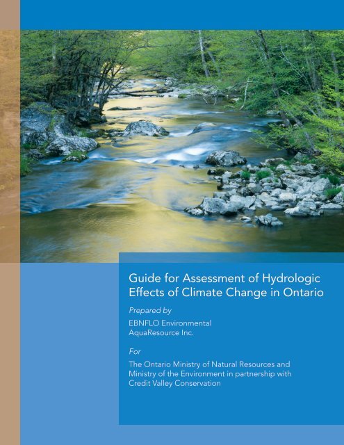
Guide for Assessment of HydrologicEffects of Climate Change in OntarioPrepared byEBNFLO EnvironmentalAquaResource Inc.ForThe Ontario Ministry of Natural Resources andMinistry of the Environment in partnership withCredit Valley ConservationJune 2010

AcknowledgementsiA large number of individuals representing a broad spectrum of agencies, organizations and technical disciplinescontributed to the development of this guidance document. The project team was comprised of the followingmembers:Team Member Affiliation Project RoleMike Garraway Ministry of Natural Resources Project DirectorRobert Walker EBNFLO Environmental Project ManagerLinda MortschEnvironment Canada, Adaptation andImpacts Research SectionTechnical Team Member, SteeringCommitteeDave Van Vliet AquaResource Inc. Technical Team Member, SteeringCommitteeSam Bellamy AquaResource Inc. Technical Team Member, SteeringCommitteeDan Banks Credit Valley Conservation Authority Project Administrator, SteeringCommitteeLynne Milford Ministry of Natural Resources Project Liaison, Steering CommitteeHugh Whiteley University of Guelph Peer Reviewer, Steering CommitteeRick Gerber Toronto and Region Conservation Authority Peer Reviewer, Steering CommitteeDave Belanger City of Guelph Steering CommitteeDon Ford Toronto and Region Conservation Authority Steering CommitteeDoug Jones Town of Orangeville Steering CommitteeJohn Kinkead Credit Valley Conservation Authority Steering CommitteeLeilani Lee-Yates Region of Peel Steering CommitteeLorrie Minshall Grand River Conservation Authority Steering CommitteeClara Tucker Ministry of the Environment Steering CommitteeJacqueline Weston Halton Region Steering CommitteeKathy Zaletnik Ministry of the Environment Steering CommitteeChristine Zimmer Credit Valley Conservation Authority Steering CommitteeDr. Don Burn from the Department of Civil Engineering, University of Waterloo was a valued advisor to the team.Mr. James Bruce provided review comments. Several other individuals attended Steering Committee meetings andoffered valuable comments and suggestions.Neil Comer, Adaptation and Impacts Research Division, Environment Canada was instrumental in making the mostrecent solar radiation data from the IPCC AR4-related Global Climate Model runs available on the CCCSN.cawebsite for use in this project.Andrea Hebb and Shaina Collin provided technical support to the project team.

Executive SummaryExecutive Summaryiii“Warming of the climate system is unequivocal“(Intergovernmental Panel on Climate Change (IPCC),2007c). A two-pronged response is required. First, thereis a need for global scale implementation of mitigationactions to prevent or slow the degree of climate changeand second, society must develop strategies to adaptto the impacts of a changing climate. Natural resourcemanagers are recognizing the potential threats ofclimate change and the need to adapt to anticipatedchanges at the local scale. As water resources arefundamentally important to humans and ecosystems,this field is often central to climate change impactassessment activities and has received much attention inrecent research.Climate change impact assessments are the first stepin mainstreaming climate change in managementand adaptation processes. Climate change impactassessment procedures have advanced to the stagewhere they can be applied by water resource scientists,engineers and planners across Ontario in a widevariety of applications. This Guide for Assessment ofHydrologic Effects of Climate Change in Ontario (theGuide) outlines a recommended climate change impactassessment procedure in the context of water resourcestudies in Ontario.Purpose of the GuideThis Guide provides a methodology for conductingassessments of the effects of climate change on waterresources in Ontario to both inform management andadapt decision making. These assessments will need toexamine system vulnerabilities; options for operations,management and adaptation; public education; andmethods to achieve robust and resilient water resourcesystems into the future. The methodology builds uponconventional water resource assessments by guiding theuser through additional stages including selecting futureclimate scenarios, acquiring information, developingfuture climate time series, using these future climates todrive hydrologic models, and assessing the simulatedimpacts. The overall objective of the Guide is toestablish a standard procedure for conducting climatechange impact assessments of hydrologic systems inOntario and thus, facilitate the mainstreaming of climatechange impact assessments.The Guide does not address the influence of climatechange on the occurrence of extreme short-durationrainfall events or on peak flow rates in detail and assuch, intensity-duration-frequency (IDF) curves arenot included in the scope of climate change impactassessments. This is because Global Climate Models(GCMs), which form the basis for the assessmentprocedures recommended in this Guide, do not simulatehigh resolution storms (i.e., thunderstorms) and thereforecannot address climate variability and the occurrence ofextreme weather events for the future. Little guidanceis available on estimating future trends in storms at thelocal scale; however, various agencies and researchersare engaged in developing IDF curves on a site specificbasis that include the influence of changing climate. Theguidance provided in this document supports studies ofwater balance, aquatic habitat and streamflow frequencythat examine the whole hydrologic cycle and itsseasonality, rather than event based stormwater – peakflow design and management.Framework for the Climate Change ImpactAssessment and Guide ContentsThe Guide adopts a seven stage framework for climatechange impact assessment, as illustrated below. The firstthree stages are common to any hydrologic assessment;the remaining stages relate specifically to climatechange.This guidance document provides background onglobal and local climate change, both in terms ofwhat has occurred and what can be expected in thefuture; offers considerations regarding climate changeand specific programs in Ontario such as drinkingwater source protection, water allocation planning,

Guide for Assessment of Hydrologic Effects of Climate Change in Ontarioivsubwatershed studies, environmental monitoring, anddam and reservoir management; discusses future climatescenarios along with GCMs and greenhouse gas (GHG)emission scenarios; identifies methods for developingfuture local climates; examines the hydrologic impactsof climate change with respect to critical hydrologicprocesses, with past studies conducted in Ontariopresented; and presents a step-by-step methodology forplanning and conducting hydrologic and climate changeimpact assessments in the final chapter.A case study, included in Appendix E, tests anddemonstrates a climate change impact assessmentconducted following the recommended methods. Thesubject area for the case study is Subwatershed 19 inthe Credit River Watershed. This area, surrounding theTown of Orangeville, is the subject of a Tier Three WaterBudget and Local Area Risk Assessment for the purposeof Source Water Protection.Observed Global Climate ChangeThe Fourth Assessment Report (AR4) of theIntergovernmental Panel on Climate Change (IPCC)stated that “[w]arming of the climate system isunequivocal, as is now evident from observations ofincreases in global average air and ocean temperatures,widespread melting of snow and ice and rising globalaverage sea level” (Intergovernmental Panel on ClimateChange (IPCC), 2007b 30). In addition to global changes,long-term continental, regional and ocean-scale changesin climate have also been observed and are reflected inchanges to arctic temperatures, ice, extremes (droughts,heavy precipitation and heat waves), and wind patterns.Moreover, the human influence extends beyond globaltemperature to other aspects of climate, includingocean warming, continental-average temperatures,temperature extremes and wind patterns.Observed global changes in climate relevant to waterresources are summarized in the following table.Observed changes in global climate relevant towater resources (Intergovernmental Panel on ClimateChange (IPCC), 2001b; Solomon et al., 2007; Bates etal., 2008)Observed Changes• Increase in the number, frequency and intensity ofheavy precipitation events, even in areas where totalprecipitation has decreased.• Decrease in snow cover in most areas of thecryosphere, especially during the spring and summermonths• Higher water temperatures in lakes.• Reductions (approximately two weeks) in the annualduration of lake and river ice cover in the mid andhigh latitudes of the Northern Hemisphere.• Increase in actual evapotranspiration from 1950to 2000 over most dry regions of the USA andRussia (greater availability of water on or near landsurface from increased precipitation and largeratmospheric capacity for water vapour due to highertemperature).• Increase in annual runoff in high latitudes andsome regions of the USA (decrease in West Africa,southern Europe and southernmost South America).• Altered river flow in regions where winterprecipitation falls as snow; more winter precipitationfalling as rain.• Earlier snowmelt, due to warmer temperatures.• Fewer numbers of frost days, cold days, cold nightsand more frequent hot days and hot nights.• Decrease in diurnal temperature range (0.07°C perdecade) between 1950 and 2004 but little changefrom 1979 to 2004 as maximum and minimumtemperatures increase at the same rate.Projected Global Climate ChangeModelling experiments exploring the sensitivity of theclimate system to rising concentrations of greenhousegases (GHGs) project an increase in the globalmean surface air temperature over the 21st century(Intergovernmental Panel on Climate Change (IPCC),

Executive Summaryv2007c). The magnitude of the warming is related tothe emission of GHGs and resultant concentrationsof those gases in the atmosphere and their radiativeforcing. The best estimate for the global averagetemperature increase for 2090-2099 relative to 1980-1999is 1.8°C to 4.0°C if all emission scenarios are considered(Intergovernmental Panel on Climate Change (IPCC),2007c).Warming is projected to be greatest over land and mosthigh northern latitudes and the least in the SouthernOcean and parts of North Atlantic Ocean. In mostareas of North America, the increase in annual meantemperature is greater than the global mean citedabove. The most warming is likely to occur in winter innorthern regions and in summer in the south westernUSA. Minimum winter temperatures are likely to increasemore than average temperatures in northern NorthAmerica.Warming generally increases the spatial variability ofprecipitation. Rainfall in the subtropics is projected todecrease and precipitation is projected to increase athigher latitudes (Christensen et al., 2007b). In Canadaand northeast USA, annual precipitation is very likelyto increase and it is likely to decrease in the southwestUSA. The seasonal distribution of precipitation is alsoaffected; winter and spring precipitation in southernCanada is likely to increase and summer precipitationis likely to decrease. The snow season length and snowdepth are expected to decrease except in northernmostCanada where the maximum snow depth will likelyincrease (Christensen et al., 2007b). The following tablelists some projected changes in global climate relevantto water.Projected changes in global climate as they relate towater (Meehl et al., 2007; Bates et al., 2008)Observed Changes• Hot extremes and heat waves will very likely be moreintense, frequent and longer in duration.• Number of frost days in middle and high latitudesdecrease and growing season lengthens.• Increased likelihood of summer drying in midlatitudesand associated risk of drought (increasingfrom 1% of present-day land area to 30% by 2100).Observed Changes• Increase in number of consecutive dry days.• Very likely that heavy precipitation events willbecome more frequent.• Increase in the amount and intensity of precipitationat high latitudes and in tropics; decreases in somesub-tropical and lower mid-latitude regions.• Area of snow cover projected to contract, glaciers/ice caps lose mass; in many areas summer melting isgreater than winter snowfall accumulation.• By 2050, permafrost area in Northern Hemispherelikely to decrease 20-35%; increases in thaw depth.• Potential evaporation projected to increase(atmosphere’s water-holding capacity increases withhigher temperatures but relative humidity stayssame); increase in water vapour deficit.• Runoff increases in high latitudes and wet tropics,decreases in mid-latitudes and some parts of drytropics.Observed Changes in Ontario’s ClimateChanges in the climate system have also been observedat the local scale – in Ontario and within the Great LakesBasin, as summarized below:• Annual average air temperatures across the provinceincreased from 0 to 1.4°C; the greatest warmingoccurred in the spring for the period 1948 to 2006,(Lemmen et al., 2008).• The number of warm days and night-time wintertemperatures increased between 1951 and 2003(Bruce et al., 2006a).• Total annual precipitation increased 5-35% since1900, (Zhang et al., 2000) and the number of days withprecipitation (rain and snow) increased (Vincent andMekis, 2006).• Water vapour in the Great Lakes Basin and SouthernOntario has increased more than 3% from 1973 to1995, contributing to higher intensity rainfall events(Ross and Elliott, 2001).

Guide for Assessment of Hydrologic Effects of Climate Change in Ontariovi• Increased night-time temperatures in the summer hasbeen linked to more intense convective activity andrainfall contributing to greater annual precipitationtotals (Dessens, 1995).• The number of strong cyclones increased significantlyacross the Great Lakes over the period 1900 to 1990(Angel and Isard, 1998).• Heavier, more frequent and intense rainfall eventshave been detected in the Great Lakes Basin sincethe 1970s.• The maximum intensity for one-day, 60-minuteand 30-minute duration rainfall events increasedon average by 3-5% per decade from 1970 to 1998(Adamowski et al., 2003).• The frequency of intense daily rain events increasedfrom 0.9% (1910 to 1970) to 7.2% (1970 to 1999) forvery heavy events and from 1.5% to 14.1% for extremeevents (Soil and Water Conservation Society, 2003) forthe same periods.• An increase in lake-effect snow has been recordedsince 1915 (Burnett et al., 2003).• Precipitation as snow in the spring and fall hasdecreased significantly in the Great Lakes-St.Lawrence basin between 1895 and 1995, althoughtotal annual precipitation has increased, (Mekis andHogg, 1999).Projected Changes in Ontario’s ClimateProjected changes in Ontario climate are based uponGCM simulations. Over 30 different GCM-scenariocombinations indicate that total annual precipitationcould increase by 2 to 6%, while temperatures couldincrease by 2 to 4ºC by the 2050s over the Great LakesBasin (Bruce et al., 2003). The greatest warming is likelyto occur in Northern Ontario during winter. Changes inextreme warm temperatures are expected to be greaterthan changes in the annual mean temperature (Kharinand Zwiers, 2005). The number of days exceeding 30°C isprojected to more than double by the 2050s in SouthernOntario (Hengeveld and Whitewood, 2005) and thenumber of severe heat days could triple in some cities bythe 2080s (Cheng et al., 2005). Heat waves and droughtmay become more frequent and long lasting.Most climate modelling results suggest that annualprecipitation totals will likely increase across Ontario;however, summer and fall precipitation amounts maydecrease up to 10% in southern portions of the Province.Winter precipitation may increase as much as 10% in thesouth and 40% in the north (Lemmen et al., 2008). Morewinter precipitation is very likely to fall as rain. Lakeeffectsnow will likely increase until the end of the 21stcentury, then snowfall may be replaced by lake-effectrainfall events (Kunkel et al., 2002; Burnett et al., 2003).Extreme rainfall events in Ontario are expected toincrease by 5% per decade while severe winter stormsincrease in intensity. Thirty minute and daily extremerainfall may increase by 5% and 3% per decade,respectively (Bruce et al., 2006b).Hydrologic Studies and Climate ChangeManagers can explore a range of adaptation strategiesthat expand the coping range of a hydrologic systemby considering the potential impacts of climate change.Since we can no longer rely on historical trends toguide our planning for the future, water resourcemanagers must look forward by examining the possibleconsequences of a wide range of plausible futureclimates. Climate change impact assessment providesinsight into future directions in terms of water resourcesystem response and behaviour.Climate change has the potential to affect both theavailability of water for municipal uses and the qualityof that water. The Clean Water Act of 2006 and theDrinking Water Source Protection program instituteda series of technical studies across the Province; theresults of these studies may be significantly altered bychanging climates. For example, more intense rainfallreduces recharge rates, more prolonged droughtincreases the need for stored water supplies, and higherevapotranspiration can reduce the amount of water inreservoirs. Water quality may be degraded by increasedaquatic plant growth instream as a result of climatechange. Also, more intense rainfall may result in greaterrates of soil and streambank erosion and transport of soilbound pollutants to streams.The Permit-to-Take-Water (PTTW) program will beaffected by changing climates. With warmer instreamwater temperatures and higher evapotranspiration,streamflow may be reduced to levels that threatenaquatic communities and water supplies. Seasonalredistribution of precipitation may result in lowerstreamflow on a seasonal basis. Water users may findtheir needs changing in the future as climates change.For example, agricultural irrigation and golf course

Executive Summaryviiwatering needs may shift earlier in the year and mayrequire more water if drought becomes more frequent.In addition to the Drinking Water Source Protectionprogram and the Permit-to-Take-Water program, severalother water related programs in Ontario are affected byclimate change. These include subwatershed studies,environmental monitoring programs, stormwatermanagement and dam/reservoir management.Hydrologic assessments can also support ecosystemand resource productivity studies in several disciplines(i.e., agriculture, forestry etc.). In all cases climate changecan cause significant changes in hydrology and waterquality that must be recognized as part of adaptivemanagement planning.Global Climate ModelsGCMs are coupled ocean-atmosphere models thatattempt to simulate future climate under alternate GHGforcing scenarios. These tools have evolved since the1970s to their present level of sophistication. Numerousmodelling centres around the world have developedGCMs that are used for long-term simulations (i.e.,250 year) to characterize the evolution of temperature,precipitation, solar radiation, winds and otherparameters well into the future. GCMs produce globalscale output at grid point spacings of 250 to 400 km.Simulations are designed to characterize future climateon an annual, seasonal and monthly basis at relativelycoarse spatial scales. GCMs do not simulate small scalestorms (i.e., thunderstorms) and therefore cannot reflectextreme events at the local scale.Greenhouse Gas Emission ScenariosA standard set of GHG emission scenarios have beendeveloped by the IPCC. These scenarios representfuture storylines based on alternative directionsfor humanity in terms of economies, technology,demographics and governance. Each scenario resultsin a different rate and timing of GHG emissions that,in turn, are developed into GHG concentrations thatdrive the GCMs to simulate a unique future climate.The different GCMs forced by alternate GHG emissionscenarios results in a large number of possible futureclimates. Since each future climate is considered equallyplausible, the IPCC recommends that climate changeimpact assessments use as many of these scenarios aspossible.Developing Future Local Climates as Input toModelling AssessmentsFuture local climates must be developed to be used asinput to hydrologic models for climate change impactassessments. Currently, all climate scenario-generatingapproaches rely upon the GCM simulations.The most established methodology for estimatingfuture local climates uses the GCM simulations toestimate annual, seasonal or monthly changes for eachclimate variable for a future time period relative to abaseline climate period. These relative changes, termedchange fields, are used to adjust the observed climatestation data time series to reflect future conditions.This approach results in an altered input climate timeseries that reflects the average relative change in eachparameter and, through the use of local observations,the local climate. The change field method is a simpleapproach to develop future local climates that reflectlarge scale average features and allows the use of allGCM and GHG emission scenarios. It is also importantto recognize the limitations of this approach; it doesnot alter the sequence of wet and dry days nor does italter the patterns of intense precipitation events. GCMslack the local scale parameterization and feedback fromlocally significant features (i.e., topography and surfacewater) to reflect local scale conditions directly in modeloutput.Climate downscaling methods have been developedto reflect local conditions and address climatevariability. Two different approaches include statisticaldownscaling and dynamical downscaling. Statisticaldownscaling methods can be further divided intoregression type models and weather generators.Statistical regression models are conceptually simpleapproaches to climate scenario generation. Resolvedatmospheric conditions at the GCM scale are linkedto climatic features or parameters at the local scalethrough statistical relationships. These tools rely uponpredictors selected from large scale (i.e., GCMs) climatemodelling output (e.g., upper atmosphere water-vapourcontent, barometric pressure or geopotential thickness).Predictors must be selected for the strength of theirinfluence on important local scale predictands, such asair temperature, precipitation, wind speed and radiation,as required in hydrologic modelling. The assumption ofstationarity, that these relationships will hold true into

Guide for Assessment of Hydrologic Effects of Climate Change in Ontarioviiithe future with climate change, is crucial to the validityof this approach. Changes in the variability of weatherin the future and weather extremes are addressed bythis method. Predictors generated by GCMs for futuretime periods reflect future climate variability and thusinfluence the variability of the predictands through theregressions. Guidance is provided on acquiring andapplying the Statistical Downscaling Model (SDSM) togenerate future climates that incorporate changes inclimate variability.Weather generators are statistically-based climatemodels that replicate the statistical attributes (i.e.,mean and variance) of local observed climate variables(Christensen et al., 2007a; Wilby et al., 2004). Weathergenerators do not replicate observed sequences ofevents; they simulate the sequence of wet and dryweather events and the transition from one to another(de Loë and Berg, 2006). Often secondary variables suchas air temperature and solar radiation are modelledconditionally on precipitation conditions, especially thepresence or absence of rain. Since weather generatorsrely on climate statistics, long observation records arerequired to develop robust scenarios. Variability ofclimate is addressed with this method as GCM simulatedfuture climate variance can be incorporated in the futureweather model formulation. The weather generatorLARS-WG is discussed in the Guide with information onacquiring and applying the model.Dynamical downscaling using regional climate models(RCMs) is one of the most promising methods fordownscaling GCM output. RCMs are physically based3-D models capable of representing important physicalfeatures (i.e., topography and water bodies) and climaticprocesses such as the formation of convective stormsand soil moisture storage over small portions of theglobe. RCMs are typically nested within GCMs anduse one-way boundary conditions such as sea-surfacetemperatures and atmospheric circulation patterns fromthe GCMs to drive them (de Loë and Berg, 2006). RCMssimulate smaller scale physical processes involvingthe use of interactive land-surface models. Output isavailable at finer resolution than from GCMs, typicallyin the range of 40 to 50 km spacing; thus, an orderof magnitude more spatially detailed than the GCMsoutput. Because of the smaller scale of the modeldomain, RCMs can simulate individual storms (notsmaller convective events such as thunderstorms) and,therefore, can be used to examine the occurrence offuture storms and extreme events.The following table describes these approaches forgenerating future climates and lists their relativeadvantages and disadvantages.Summary GCM-change field and downscaled climates for use in climate change impact assessmentsTechnique Description Advantages DisadvantagesGCM-change fieldSummary GCM continued next page• Simulated climate at coarsegrid spacing• Use to develop monthly(seasonal or other) changefields• Provides data used instatistical downscaling• Wide variety of GCMsavailable• Several GCMs have beenapplied to long-termsimulations for family ofemission scenarios• Comprehensive physicallybased tools• Several variables available• Good agreement acrossGCMs on temperaturechange• Coarse spatial resolution,unrepresentative of localclimate• Extreme events generallyoccur at a smaller scale thanGCM scales, not represented• Modest agreement acrossGCMs on precipitation• Cannot be used to changeclimate variability

Executive SummaryixSummary GCM continuedTechnique Description Advantages DisadvantagesStatistical Downscalingwith RegressionWeather GeneratorsRegional Climate Models• Climates based uponstatistical relationshipsbetween climate variablesand atmospheric predictors• Weather data generatedbased on statistical attributesof local climate and GCMvariables• Higher resolution physicallybased models oftenembedded in GCMs• Local physiography andwater bodies are included• High spatial and temporalresolution if observationaldata available• Several variables available• Ease of application, thusmany long-term scenarioscan be tested• Good skill demonstrated atsimulating temperature• High spatial and temporalresolution if observationaldata available• Several variables available• Ease of application, thusmany long-term scenarioscan be tested• Good skill demonstrated atsimulating temperature• Good skill at simulatingperiods of drought andextended precipitation• High spatial and temporalresolution output for severalvariables• Improved extreme eventsimulation over GCMs• Physically based andconsistent with GCMs• May account for feedbackfrom anthropogenic ornatural systems• Assumes empiricalrelationships will hold asclimates change• May perpetuate GCM biases• Generally underestimatesextremes• Some models do notsimulated monthly variabilitywell• Poor skill in simulatingprecipitation extremes• Neighbouring stations notcorrelated• Observational data to buildstatistical relationships notavailable in all areas• Assumes empiricalrelationships will hold asclimates change• May perpetuate GCM biases• Generally underestimatesextremes• Some models do notsimulated monthly variabilitywell• Poor skill in simulatingprecipitation extremes• Neighbouring stations notcorrelated• Observational data notavailable in all areas• Few model runs and GHGemission scenarios available• May perpetuate GCM biases• Complex model systemsprecludes non-expert use• Simulation periods aretypically short, thus fewerextremes are representedCritical Hydrologic ProcessesThe Guide discusses critical hydrologic processes andthe influence of climate variables on the function ofthese processes. Evapotranspiration, winter conditions(i.e., snow cover, frozen ground), groundwater recharge,and streamflow are discussed with respect to theirsensitivity to climate change. Recommendations aremade with respect to the selection of appropriateclimate sensitive hydrologic formulations. SeveralOntario-based studies of the impact of climate changein hydrologic systems are highlighted with respect totheir methods and conclusions.Climate Change Impact AssessmentThe final chapter in the Guide provides a step-by-stepprocedure for conducting a hydrologic climate changeimpact assessment. A Step-by-Step Guide to HydrologicAssessment Incorporating Climate Change, presented in

Guide for Assessment of Hydrologic Effects of Climate Change in Ontarioxthe following section, tabulates the major steps involvedin conducting a hydrologic assessment incorporatingclimate change.The climate change impact assessment steps include:1. Definition of Problem. This stage is designed to helpestablish the scope of work and the organization ofinformation. It consists of a statement of goals andobjectives, and identification of primary issues andconcerns in the study area; identification of spatialand temporal factors for the study; and a preliminarylisting of data and information needs and sources.2. Select Hydrologic Modelling Methods. This taskincludes the identification of a general hydrologicmodelling approach and the selection of specificmodelling tools. Alternative approaches include theuse of simple to complex streamflow models, linkedstreamflow and groundwater models and coupledor conjunctive models. Modellers must determinethe most appropriate type of streamflow modeland whether groundwater modelling is warranted.Individual hydrologic process models are discussedwith special emphasis on their relevance to climatechange impact assessments.3. Model Setup and Testing. This stage involves dataacquisition, model setup, calibration and validation,and discussion of errors and confidence.4. Select Climate Scenarios. There are numerousGCMs and GHG emission scenarios to choosefrom when conducting a climate change impactassessment. The challenge is to select a subset ofscenarios that represents the larger group, such thatthe level of effort is minimized without sacrificinginformation. A scenario selection method (termedthe Percentile Method) is proposed that provides arationale for selecting GCM - GHG scenarios that arerepresentative of the full set of scenarios availableto the user. The percentile method selects up to10 scenarios on a statistical basis such that five areselected because they represent the 5th, 25th, 50th,75th and 95th percentiles of annual temperaturechange. A second set of five scenarios are chosenat the same statistical levels based on annualprecipitation change. It is possible that one scenariosatisfies more than one criterion and less than 10scenarios in total are selected. This subset of climatescenarios represents the full range of predicted futureclimates and therefore can be used to investigate thecentral tendency among the group of climates as wellas the effect of the more extreme climates (i.e., 5thand 95th percentiles).5. Develop Future Local Climates. Guidance is providedon data acquisition and manipulation, scenarioselection and processing and methods for comparingclimates. It is recommended that climate changeimpact assessments include the following future localclimate scenarios:• Ten GCM change field climates (PercentileMethod);• At least one statistical regression climate usingSDSM;• At least one weather generator climate usingLARS-WG;• The corresponding GCM change field climatesused to generate the SDSM and LARS-WGclimates; and• At least one RCM-based future climate.6. Assessment of Hydrologic Impacts. A procedureis proposed for reviewing simulation results andcomparing current and future conditions. Thefollowing steps are recommended:• Identify reference regime;• Select metrics and identify standards/targets;• Setup future climate model scenario;• Model climate change impacts by scenario;• Compare changes in climates;• Compare hydrologic changes by scenario; and• Consider uncertainty.This section offers an approach to interpreting resultsfrom the full suite of scenarios and dealing withuncertainty. The range of outcomes and the prevailingtrends provide valuable indications of likely futureconditions and necessary coping ranges.7. Recommendations. Suggestions are provided onthe formulation of recommendations. These includerecommendations to fill data gaps, to conduct futurestudies, and to monitor and identify future adaptationmeasures.

Executive SummaryxiStep-by-step Guide to Hydrological AssessmentIncorporating Climate ChangeThis section provides a condensed version of themajor steps involved in conducting a hydrologicassessment incorporating climate change. This list mayserve as a checklist to guide project planning. A moredetailed version is provided in Chapter 6 (Chapter 6section numbers correspond to the steps in this table),with necessary supporting material included in theappendices. The Guide provides a perspective andrationale for the recommended procedures. Areaswhere improved techniques are being developed areidentified.Assessment of the hydrological effects of climatechange is a challenging technical endeavour in an areaof rapidly-expanding knowledge. Hydrologists andmodellers who intend to conduct a climate changeanalysis of their watershed should first become familiarwith all of the material in this document. Properlyused, the existing assessment techniques describedin this Guide provide a good basis for developmentof adaptation strategies. Nevertheless, due diligencerequires that modellers remain in close touch withresearch findings and incorporate improved techniquesas they become available.Modelling andConsiderations/TasksCommentsAssessment Steps1. Definition of Problem Identify goals and objectives Section 6.1.1 lists seven commonly chosen goalsand objectivesDelineate study areaInclude surface and subsurface domainsIdentify hydrologic issues and concerns Specify targets, communities and water useactivities at risk, known trends and prevalentstresses and stressors in the systemDefine temporal aspects of analysisInclude modelling time step, model testingperiod and future time horizons2. Select ModellingMethods3. Model Setup andTesting4. Select Future ClimateScenariosDevelop an inventory of anticipated data andinformation needsConsider alternative approaches and selectpreferred approachReview models input requirementsReview hydrologic processesReview output capabilitiesReview documentation, technical support andcostsAcquire and organize information and data As listed in Step #1Setup model for study areaCalibrate and validateEstimate confidenceStep-by Step continued on next pageEstablish baseline climateInclude a list of anticipated gaps and measuresneeded to fill gapsSimple vs. complex models, single model vs.two models, linked vs. conjunctive modelsQuestion whether needs can be met and criticalgaps filled.Question whether the model uses algorithms forkey processes that can accurately represent thesensitivity of the process to climate change.Review the degree to which the model producesthe necessary information for assessment.Can the model be run by available staff andproduce results within required timelines andbudget?Level of detail and resolution must match outputexpectations and objectivesFully test models abilities by season andweather conditionIdentify sources of uncertainty and overall skillof modelGenerally 1961 to 1990 for GCM and similarperiod or longer for the current climatologicalbaseline

Guide for Assessment of Hydrologic Effects of Climate Change in OntarioxiiStep-by Step continuedModelling andAssessment Steps5. Select and ApplyClimate Methods toDevelop Future LocalClimates6. Assessment ofHydrologic Impacts ofClimate ChangeConsiderations/TasksDownload GCM temporal dataDetermine GCM/SRES scenario suiteProcess monthly GCM temporal data anddevelop monthly change fieldsAlter existing weather data set to reflectchange fieldsDownload daily predictor, GCM and RCMdata sets, for current and future conditions fordownscalingGenerate future climates using statistical modeland weather generator (if possible)Process RCM data to create future climate dataset (if possible)Create evapotranspiration time series for allscenariosIf necessary process daily data to obtain datafor sub-daily time stepsCompare future climates to baseline climateDesign Assessment Scenarios and FutureConditionsModel hydrologic scenariosCompare hydrologic conditions and climatesCompare hydrologic changes in aggregateAssess overall uncertaintyCommentsTemperature and PrecipitationDetermine how many and which scenarios toapplyAt least temperature and precipitation andpossibly, solar radiation, wind and humidityBasis of future climateRepeat for each scenarioRepeat for each scenario desiredEvapotranspiration should be sensitive to futureclimateLand use, management practices, water usageand other factors should reflect future timehorizons studiedTabulate and compare in hydrological andmeteorological terms and identify causes ofchangeConsider all consequences in hydrologicallyinfluenced systemsBased on suite of scenario outcomes7. Recommendations Mitigation and adaptation Identify potential mitigation and adaptationmeasuresFuture studiesList studies to fill gaps, extend data basethrough monitoring and improve modelling andtechnical capacity

Table of ContentsTable of ContentsxiiiAcknowledgements..................................................................................................................................................................iExecutive Summary................................................................................................................................................................. iiiTable of Contents.................................................................................................................................................................. xiii1 Introduction.......................................................................................................................................................................11.1 Purpose and Objectives......................................................................................................................................21.2 Target Users and Applications...........................................................................................................................21.3 General Approach...............................................................................................................................................31.4 Guide Layout.......................................................................................................................................................42 Background........................................................................................................................................................................52.1 Global Climate Change – The Big Picture........................................................................................................52.1.1 What’s Happening Globally..................................................................................................................52.1.2 What to Expect in the Future...............................................................................................................62.2 What’s Happening Locally in Ontario..............................................................................................................102.2.1 Changes We’ve Experienced.............................................................................................................102.2.2 Ontario’s Future Climate.....................................................................................................................112.3 Considerations for Climate Change Impact Assessments in Ontario..........................................................122.3.1 Drinking Water Source Protection.....................................................................................................142.3.2 Water Demand Estimates and Water Allocation Planning..............................................................142.3.3 Subwatershed Planning......................................................................................................................152.3.4 Environmental Monitoring Programs.................................................................................................152.3.5 Stormwater Management...................................................................................................................152.3.6 Dams/Reservoirs..................................................................................................................................173 Future Climate Scenarios...............................................................................................................................................193.1 Global Climate Models (GCMs).......................................................................................................................193.2 GHG Emission Scenarios..................................................................................................................................224 Estimating Future Local Climates..................................................................................................................................274.1 GCM-Based Scenarios......................................................................................................................................274.2 Synthetic and Analogue Scenarios..................................................................................................................284.2.1 Synthetic Scenarios.............................................................................................................................284.2.2 Analogue Scenarios............................................................................................................................284.3 Downscaling.......................................................................................................................................................294.3.1 Statistical - Regression........................................................................................................................304.3.2 Statistical - Weather Generators........................................................................................................314.3.3 Dynamical - Regional Climate Models (RCMs).................................................................................324.4 Summary of Local Climate Generation Techniques.......................................................................................335 Hydrologic Impacts.........................................................................................................................................................355.1 Studies Completed in Ontario.........................................................................................................................355.1.1 Credit Valley Conservation (CVC) (Walker and Dougherty, 2008)....................................................355.1.2 Toronto Region Conservation Authority (TRCA) (Walker, 2006).......................................................375.1.3 Grand River Conservation Authority (GRCA) (Bellamy et al., 2002).................................................375.1.4 Hydrologic Models for Inverse Climate Change Impact Modelling(Upper Thames River Basin) (Cunderlik and Simonovic, 2005, 2007)..............................................385.1.5 The Impact of Climate Change on Spatially Varying Groundwater Rechargein the Grand River Watershed (Ontario) (Jyrkama and Sykes, 2007)...............................................395.2 Hydrologic Processes........................................................................................................................................395.2.1 Evapotranspiration..............................................................................................................................395.2.2 Winter Conditions...............................................................................................................................415.2.2.1 Frozen Soil..............................................................................................................................415.2.2.2 Snow.......................................................................................................................................415.2.3 Groundwater Recharge.......................................................................................................................43

Guide for Assessment of Hydrologic Effects of Climate Change in Ontarioxiv5.2.4 Streamflow...........................................................................................................................................445.2.5 Water Quality.......................................................................................................................................456 Climate Change Assessment.........................................................................................................................................476.1 Define Problem..................................................................................................................................................476.1.1 Goals and Objectives..........................................................................................................................476.1.2 Issues and Concerns............................................................................................................................476.1.3 Spatial Considerations........................................................................................................................486.1.4 Temporal Considerations....................................................................................................................486.1.5 Resource Needs – Data and Information..........................................................................................496.1.6 Summary...............................................................................................................................................496.2 Select Hydrologic Modelling Methods...........................................................................................................506.2.1 Select Water Resources Modelling Approach..................................................................................506.2.1.1 Streamflow Generation Model.............................................................................................506.2.1.2 Linked Streamflow Generation and Groundwater Models................................................506.2.1.3 Coupled or Conjunctive Models..........................................................................................516.2.1.4 Modelling Approach Selection.............................................................................................516.2.2 Select Water Resources Model..........................................................................................................516.2.2.1 Input Requirements...............................................................................................................526.2.2.2 Identify Key Hydrological Processes and Methods............................................................526.2.2.3 Required Output....................................................................................................................566.2.2.4 Hydrologic Model Price, Support, and Documentation....................................................576.2.3 Summary...............................................................................................................................................576.3 Model Setup and Testing.................................................................................................................................576.3.1 Data Acquisition and Setup................................................................................................................576.3.2 Calibration/Validation.........................................................................................................................576.3.3 Determine Errors and Confidence.....................................................................................................586.3.4 Summary...............................................................................................................................................596.4 Select Climate Scenarios..................................................................................................................................596.4.1 Define Baseline Climate or Current Conditions................................................................................606.4.2 Select GCM Scenario Suite.................................................................................................................616.4.2.1 Vintage of the GCM..............................................................................................................616.4.2.2 Type of GHG Emission Scenario...........................................................................................626.4.2.3 Performance of GCMs in Replicating Current Climate......................................................646.4.2.4 Availability of Critical Atmospheric Parameters for the HydrologicAssessment Application........................................................................................................646.4.2.5 Selection of Baseline Period and Future Time Period for the GCM Component............646.4.3 Selecting the Number of Climate Change Scenarios......................................................................656.4.3.1 Scatter Plot Method - ‘Bounding the Uncertainty’.............................................................666.4.3.2 Percentiles Method...............................................................................................................666.4.3.3 Analysis of Results..................................................................................................................726.4.3.4 Recommended Approach to Scenario Selection...............................................................726.4.4 Determine Independent Factors for Future Scenarios.....................................................................776.4.5 Summary...............................................................................................................................................776.5 Develop Future Local Climates........................................................................................................................776.5.1 Overview...............................................................................................................................................776.5.2 GCM Change Fields............................................................................................................................786.5.3 Statistical Downscaling Method.........................................................................................................806.5.4 Weather Generator Method...............................................................................................................826.5.5 Regional Climate Model.....................................................................................................................846.5.6 Disaggregate Daily Data and Potential Evapotranspiration Generation.......................................85

Table of Contentsxv6.5.7 Compare Alternative Climates...........................................................................................................866.5.8 Summary...............................................................................................................................................866.6 Assessment of Hydrologic Impacts..................................................................................................................876.6.1 Identify Reference Regime.................................................................................................................876.6.2 Select Metrics and Identify Standards...............................................................................................876.6.3 Setup Future Conditions Model(s).....................................................................................................896.6.4 Model Climate Change Impacts by Scenario...................................................................................896.6.5 Compare Changes in Climate Data...................................................................................................906.6.6 Compare Hydrologic Changes by Scenario......................................................................................906.6.7 Consider Uncertainty...........................................................................................................................926.6.8 Summary...............................................................................................................................................946.7 Recommendations............................................................................................................................................946.7.1 Filling Gaps..........................................................................................................................................946.7.2 Future Studies......................................................................................................................................956.7.3 Monitoring...........................................................................................................................................956.7.4 Adaptation...........................................................................................................................................956.7.5 Summary...............................................................................................................................................95Bibliography...........................................................................................................................................................................97Appendix A – Watershed and Receiving Water Model CapabilitiesAppendix B – GCM Modelling GroupsAppendix C – GCM-based Change Field Assessment and Hydrologic ModellingAppendix D – RCM and GCM Data ConversionAppendix E – Subwatershed 19 Case StudyList of FiguresFigure 1.1 Climate change impact assessment steps.....................................................................................................3Figure 2.1 Estimated probabilities for a mean surface temperature change exceeding 2°C in 2080 to 2099relative to 1980 to 1999 under the mid-range GHG emission scenario (SRES A1B scenario).Results are based on a single GCM (a, c), and a multiple GCM mean (b, d), for winter (a, b) andsummer (c, d). ((Meehl et al., 2007 811) Climate Change 2007: The Physical Science Basis.Working Group I Contribution to the Fourth Assessment Report of the Intergovernmental Panelon Climate Change, Figure 10.30. Cambridge University Press).................................................................7Figure 2.2 Temperature and precipitation changes (between 1980 to 1999 and 2080 to 2099) for NorthAmerica averaged for 21 GCMs for the mid range emission scenario (i.e., A1B) ((Christensen etal., 2007b 890) Climate Change 2007: The Physical Science Basis. Working Group I Contributionto the Fourth Assessment Report of the Intergovernmental Panel on Climate Change, Figure11.12. Cambridge University Press)................................................................................................................8Figure 2.3 Schematic of coping range (Lemmen and Warren, 2004)..........................................................................13Figure 2.4 Adaptive measures to increase coping range (Lemmen and Warren, 2004)............................................13Figure 2.5 Example reservoir rule curve Grand River Conservation Authority (data source athttp://www.grandriver.ca/index/document.cfm?sec=2&sub1=0&sub2=0)..............................................17Figure 3.1 Conceptual structure of a coupled atmosphere-ocean general circulation model(Viner and Hulme, 1997)................................................................................................................................20Figure 3.2 Development of climate models through incorporation of new components/processes(Albritton et al., 2001) Climate Change 2001: The Scientific Basis. Contribution of WorkingGroup I to the Third Assessment Report of the Intergovernmental Panel on Climate Change,Box 3, Figure 1. Cambridge University Press)..............................................................................................21

Guide for Assessment of Hydrologic Effects of Climate Change in OntarioxviFigure 3.3Figure 5.1Figure 6.1Figure 6.2Figure 6.3Figure 6.4Figure 6.5Figure 6.6Figure 6.7Figure 6.8Figure 6.9Figure 6.10Figure 6.11Fossil CO 2, CH 4and SO 2emissions for six illustrative SRES non-mitigation emission scenarios,their corresponding CO 2, CH 4and N 2O concentrations, radiative forcing and global meantemperature projections based on an SCM tuned to 19 atmosphere-ocean GCMs(Meehl et al., 2007, 803).................................................................................................................................24Monthly change fields for precipitation and air temperature for 2050s in the Credit RiverWatershed as projected by two GCMs (CGCM2 and HadCM3)................................................................36Climate change impact assessment steps...................................................................................................47Left Panel: Global GHG emissions without climate policies using six illustrative SRES scenarios(coloured lines) Right Panel: Solid lines are multi-model global averages of surface warming forscenarios A2, A1B and B1, shown as continuations of the 20th-century simulations. The pink line isnot a scenario, but is for AOGCM simulations where atmospheric concentrations are held constantat year 2000 values. The bars at the right of the figure indicate the best estimate (solid line withineach bar) and the likely range assessed for the six SRES marker scenarios at 2090-2099. Alltemperatures are relative to the period 1980-1999. (Intergovernmental Panel on Climate Change(IPCC), 2007c 7) (Intergovernmental Panel on Climate Change (IPCC), 2007d 7)....................................63Scatter plot of GCM-based mean annual temperature change versus mean annual precipitationchange – 2050s relative to 1961-1990..........................................................................................................71Mean annual water balance estimates from 4 future climates (scatter plot method candidates)..........73Mean annual water balance estimates from 8 future climates (percentile method candidates).............74Mean annual water balance estimates from 57 future climates.................................................................75Mean monthly runoff for silty soils (2050s) for three scenario screening approaches..............................76Histograms illustrate the range of model predictions and likely outcomes.............................................91Flow exceedance charts illustrate the range of flows predicted for each scenario.................................92Histogram of estimated 7Q 20streamflow using 57 climate change scenarios.........................................93Range of Variability of Estimated Streamflow.............................................................................................94List of TablesTable 2.1 Observed changes in global climate relevant to water resources (Bates et al., 2008;Intergovernmental Panel on Climate Change (IPCC), 2001b; Solomon et al., 2007).................................5Table 2.2 Projected changes in global climate for 2090-2099 relative to 1980-1999 using two emissionscenarios (Intergovernmental Panel on Climate Change (IPCC), 2007d)....................................................6Table 2.3 Projected changes in global climate as they relate to water (Bates et al., 2008;Meehl et al., 2007)............................................................................................................................................9Table 2.4 Projected changes in extreme events and their likelihood of occurring(Christensen et al., 2007b).............................................................................................................................10Table 2.5 Climate changes observed and projected for Canada (as summarized in (Bruce et al., 2006b).............12Table 3.1 Characteristics of the SRES storylines (Carter et al., 2007; Nakicenovic et al., 2000)...............................23Table 4.1 Summary of general advantages and disadvantages of GCM-change field, synthetic, analogueand downscaled climates for use in assessments.......................................................................................34Table 5.1 Water Quality Effects of Climate Change....................................................................................................45Table 6.1 Emission scenarios used as “forcings” in the GCM runs for the IPCC AR4..............................................62Table 6.2 The six SRES illustrative scenarios and the stabilization scenarios (parts per million CO 2)they most resemble (IPCC-TGICA et al., 2007; Swart et al., 2002).............................................................63Table 6.3 Scenarios from the Scatter Plot Method .....................................................................................................66Table 6.4 Climate scenarios and rank of mean annual change in temperature and precipitation forthe Percentile Method...................................................................................................................................67Table 6.5 Scenarios selected by the percentiles method using mean annual temperature change field ( o C).......70

Executive SummaryxviiTable 6.6 Scenarios selected by the percentiles method using mean annual precipitation change field (%).......70Table 6.7 Climate parameters and change field operations to develop climate change scenarios.......................79Table 6.8 Climate data summary statistics...................................................................................................................86Table 6.9 Summary of hydrologic change metrics......................................................................................................88Table 6.10 Example comparison of hydrologic metrics for climate change scenarios...............................................91

Introduction1. Introduction1“Climate change impact, adaptation and vulnerability(CCIAV) assessment has now moved far beyond its earlystatus as a speculative, academic endeavour… This ispropelling CCIAV assessment from being an exclusivelyresearch-oriented activity towards analytical frameworksthat are designed for practical decision making” (Carteret al., 2007 161).Climate change, as evidenced by warming and otherrelated effects, is now an unequivocal fact in our time(Intergovernmental Panel on Climate Change (IPCC),2007c). Society needs to respond to climate change ontwo levels: by adapting to the impacts of a changingclimate; and by implementing mitigation actions at theglobal-scale to prevent or slow the degree of climatechange. Currently, natural resource managers areadapting to anticipated change in many disciplinesat the local scale. Water resources are of fundamentalimportance to humans and ecosystems; as such, thisdiscipline is often central to these activities and hasreceived much attention in recent research. Thatresearch has concentrated on improving climate changeimpact assessment methods as well as delineating futurepotential impacts.Quantifying the hydrologic effects of climate change,through climate change impact assessments, are the firststep in mainstreaming climate change in the planningprocess and thus, beginning the adaptation process.Climate change impact assessment procedures haveadvanced to the stage where they can be applied bywater managers and planners across Ontario. Waterresource impact assessments related to climate changecan be integrated into a variety of water managementaspects, including Drinking Water Source Protection,the watershed planning process, Permit To Take Water(PTTW) applications, and subwatershed studies.Projected changes in hydrology need to inform decisionmaking and planning through adaptation strategydevelopment and risk based assessment.This Guide for Assessment of Hydrologic Effects ofClimate Change in Ontario (the Guide) is intended foruse by water resource scientists, engineers and plannersin conducting climate change impact assessments.It outlines a recommended climate change impactassessment procedure for water resource studies inOntario. The procedure is designed for applicationsranging from screening level to complex water resourceassessments. Water resource and climate models aredefAdaptation • adjustment in natural or humansystems in response to actual or expectedclimatic stimuli or their effects, which moderatesharm or exploits beneficial opportunities; thereare various types of adaptation, includinganticipatory, autonomous and plannedadaptation.Mitigation • an anthropogenic intervention toreduce the anthropogenic forcing of the climatesystem; includes strategies to reduce greenhousegas sources and emissions and enhancinggreenhouse gas sinks.Vulnerability • degree to which a systemis susceptible to, and unable to cope with,adverse effects of climate change, includingclimate variability and extremes; function of thecharacter, magnitude, and rate of climate changeand variation to which a system is exposed, itssensitivity, and its adaptive capacity.Impact Assessment • practice of identifying andevaluating, in monetary and/or non-monetaryterms, the effects of climate change on naturaland human systems (Intergovernmental Panel onClimate Change (IPCC), 2007a).central to this discussion. The Guide steps throughdecisions involved in selecting and developing futureclimate change scenarios and the procedures neededto generate time series of climate variables (i.e., airtemperature, precipitation, wind speed, solar radiation,etc.) representing future time horizons (i.e., 2020s, 2050s,2080s) for hydrologic model input. Other independentfactors that must be considered when designing futurescenarios are also addressed. Background informationconcerning global climate change, climate changein Ontario and the influence of climate change onhydrologic processes is provided for context.1.1 Purpose and ObjectivesThe purpose of this Guide is to provide a methodologyfor conducting assessments of the effects of climate

Guide for Assessment of Hydrologic Effects of Climate Change in Ontario2change on water resources in Ontario. This processbuilds upon conventional water resource assessmentsby guiding the user in the selection of future climatescenarios, acquiring relevant information, developingfuture climate time series from this information, andusing these future climates to drive hydrologic models.It is assumed that users of this Guide are familiar withhydrologic modelling procedures and are experiencedwith the use of one or more surface water and/orgroundwater models. In this document, hydrologicmodels refer to surface water and groundwater models.The overall objective is to establish a standardprocedure by which water resource scientists andplanners can generate climates to reflect plausible futureconditions under a changing climate and input theseto hydrologic models for the purpose of simulatingsystem response and behaviour. Ultimately, this typeof information is essential for identifying vulnerabilitiesin the system, identifying options for control andadaptation, educating the public, and developingcomprehensive and integrated adaptive managementprograms in many related disciplines. In addition, acommon approach allows for inter-study comparisons,possible data sharing and added efficiencies.The recommendations provided in this document weretested in a case study as part of this project. The CaseStudy involved a full scale test and demonstration of theproposed methodologies in a study area encompassingSubwatershed 19 in the headwaters of the Credit RiverWatershed. Whenever possible, the case study resultswere used to support the recommendations in thisGuide.1.2 Target Users and ApplicationsThe Guide for Assessment of Hydrologic Effectsof Climate Change in Ontario is meant for use byengineers, scientists and planners involved in themanagement of water resource systems in Ontario; itcomplies with the Clean Water Act and the Canada-Ontario Agreement on the Great Lakes. This Guideprovides the step-by-step procedures to setupand conduct assessments using the best availabletechnology and most recent climate change information.This Guide is targeted towards studies that focus onwater balance and supply issues, rather than peak orextreme flows, including studies addressing:• Drinking Water Source Protection;• Permits To Take Water (PTTW) and other waterallocation studies;• Environmental monitoring programs;• Subwatershed studies;• Stormwater management (SWM) Master Plans; and• Dam and reservoir supply and yield studies.The Guide may also be applied to a variety of otherinvestigations in which hydrology plays a supportingrole, using the same fundamental approach as usedin purely hydrologic assessments. For example, suchstudies could include:• Great Lakes studies (Canada-Ontario Agreement,COA);• Remedial action plans (RAPs);• Wetlands/aquatic wildlife studies;• Lakewide Management Plans (LaMPs);• Forest management studies;• Fisheries studies;• River-effluent assimilative capacity determinations;• Aquatic mixing zone/zone of impact studies;• Control and management of navigable waterways(i.e., Great Lakes connecting channels, Trent-Severnand Rideau waterways); and• Agricultural productivity studies.The Guide does not cover the specific techniquesneeded by proponents to assess the effects ofclimate change on the intensity, duration andfrequency (IDF) of rainfall and precipitation events.Some types of hydrological studies, including thoseassociated with floodplain management or planningand analysis of stormwater infrastructure, requirethe calculation of peak catchment or watershed flowusing event-based or continuous modelling with shorttime steps. The approach described in this Guide forconducting climate change impact assessments on waterresources is not intended for these types of studies. Asdescribed in subsequent sections, while the intensity andfrequency of extreme precipitation events is expectedto increase in the future as a result of climate change,climate researchers are currently unable to reliablyquantify the magnitude, timing or character of theseshifts. As these types of changes to the precipitationregime will have impacts on all aspects of hydrologicresponse, from peak flows to annual water budgets, itwill be important to monitor developments in climate

Introduction3change research and incorporate new understandingof the future distribution and intensity into impactassessments as it becomes available.is meant to be generic, it is suited to water resourceinvestigations with some minor modifications.Undoubtedly, there will be considerable adjustmentrequired in treatment of input data and in choice ofhydrologic modelling procedures in order to incorporateconsiderations of climate change into hydrologicstudies in which potential future changes to the intensityand frequency of storms and extreme precipitationevents are of concern. Estimates of future intensity andfrequency characteristics are likely to be determinedusing a combination of risk assessment techniques andtrend analysis; whereas, the future climates determinedusing the guidance provided in this document arebased upon deterministic modelling using sophisticatedGCMs.Some aspects of stormwater management,subwatershed studies, and dam safety and operationsstudies require investigation of peak storm flows andfrequencies/risks; however, this aspect is not addressedby the guidance provided in this document. This Guidefocuses on methods and procedures for developingfuture climates that can be used as input to continuousstreamflow generating and groundwater flow modelsthat address water balance and streamflow issues.The Guide recommends the application of climatedownscaling techniques that investigate climatevariability. However, at this time, the availability ofnecessary online climate data and the general widedisparity among simulation results using these climatedownscaling techniques, especially with respect to futureprecipitation patterns, precludes widespread adoptionof downscaling for the purpose of refining futurerainfall characteristics. As such, in this Guide, the use ofdownscaling techniques is recommended only as a firstestimate of potential future climate variability. In thisregard, the downscaled climates are not recommendedfor use in studies where the subject of investigationis the future intensity and frequency of extremeprecipitation events and the resulting streamflow.1.3 General ApproachThe Intergovernmental Panel on Climate Change (IPCC)provides guidelines for conducting assessments ofclimate change impact and adaptation strategies (Carteret al., 1994; IPCC-TGICA et al., 2007). Since the approachFigure 1.1 Climate change impact assessment stepsThe approach proposed in this Guide is shown in Figure1.1. Each step is developed and explained in Chapter 6,with references to the relevant subsections in this figure.The assessment process should be formalized, as shown,to ensure that decisions allow for balancing objectiveswith capabilities and for rationalizing uncertainty giventhe resolution and level of effort. In many studies,several of the steps in this approach would already becompleted and the steps relating specifically to climatechange impact assessment (i.e., steps 4 through 7)need only be applied. However, it is good practice in allassessments to review each step.The process includes feedback loops as indicatedin Figure 1.1. The first return loop at the third stepwould be followed when an approach is found to beunsuccessful or otherwise unsuitable at the hydrologicmodel testing step. The second return loop at the sixthstep would be followed when additional or differentscenarios are required or when the assessment hasnot achieved all of the objectives and a revised ordifferent approach is required. The last loop followingrecommendations and follow-up could representsituations where recommendations include anotherassessment with a new set of objectives or at least anew set of scenarios.

Guide for Assessment of Hydrologic Effects of Climate Change in Ontario41.4 Guide LayoutThe Guide is organized to provide the user with thenecessary background information on climate change;a rationale for conducting climate change impactassessments; methods for developing scenarios; and astepwise guide through the assessment process. Thelayout of the Guide is as follows:• Chapter 2 sets the context by describing observedand projected climate change on a global andregional scale along with a limited set of climatechange studies conducted in Ontario;• Chapter 3 describes Global Climate Models (GCMs)and the greenhouse gas (GHG) emission scenarioswhich are used as the drivers to assess the responseof the climate system;• Chapter 4 outlines methods for developing localfuture climates (climate change scenarios) from theGCM runs and downscaling methods;• Chapter 5 summarizes potential hydrological impactsof climate change in Ontario; and• Chapter 6 recommends a step-by-step climatechange impact assessment procedure for hydrologicalstudies in Ontario.

Background2. Background5The Fourth Assessment Report (AR4) of theIntergovernmental Panel on Climate Change (IPCC)stated that “[w]arming of the climate system isunequivocal, as is now evident from observations ofincreases in global average air and ocean temperatures,widespread melting of snow and ice and rising globalaverage sea level” (Intergovernmental Panel onClimate Change (IPCC), 2007b 30). In addition to globalchanges, long-term continental, regional and oceanscalechanges in climate have also been observed andare reflected in changes to arctic temperatures, ice,extreme weather events (droughts, heavy precipitationand heat waves) and wind patterns. Since the mid-20thcentury, most of the observed increase in global averagetemperatures is very likely due to the observed increasein anthropogenic greenhouse gas concentration(Intergovernmental Panel on Climate Change (IPCC),2007c). This human influence extends beyond globaltemperature to other aspects of climate, includingocean warming, continental-average temperatures,temperature extremes and wind patterns. This is strongevidence that climate change is a real and presentthreat.defClimate change • change in the state of theclimate that can be identified (e.g., by usingstatistical tests) by changes in the mean and/orthe variability of its properties, and that persistsfor an extended period, typically decades orlonger. Climate change may be due to naturalinternal processes or external forcings, orto persistent anthropogenic changes in thecomposition of the atmosphere or in land use(Baede et al., 2007)2.1 Global Climate Change – The Big Picture2.1.1 What’s Happening GloballyGlobal average annual surface temperature increased0.74°C between 1906 and 2005 (Intergovernmental Panelon Climate Change (IPCC), 2007c). Eleven of the twelvewarmest ranked years on record occurred between 1995and 2006 while the two warmest were 2005 and 1998(Intergovernmental Panel on Climate Change (IPCC),2007c). Geographically, temperatures have increasedthe most in northerly latitudes with average arctictemperatures increasing at a rate more than twice theglobal rate over the last 100 years. Also, temperaturesover land areas have warmed at a faster rate than overoceans (Intergovernmental Panel on Climate Change(IPCC), 2007b). In over 70% of the land regions wheredata are available, the observed number of warmextremes has increased and the number of daily coldextremes has decreased. In the Northern Hemisphere,the greatest increase has occurred in winter and spring.Precipitation increased 0.5-1% per decade in the20th century over most land areas in the NorthernHemisphere (between 30°N and 85°N) and 0.2-0.3%per decade in the tropics (10°N and 10°S) during thisperiod. Rainfall decreased 0.3% per decade in thenorthern subtropics (10°N and 30°N) over the past 30to 40 years (Bates et al., 2008; Trenberth et al., 2007).The area affected by drought has expanded since the1970s (Solomon et al., 2007). Observed global changesin climate relevant to water resources are summarized inTable 2.1.Table 2.1 Observed changes in global climaterelevant to water resources (Bates et al., 2008;Intergovernmental Panel on Climate Change (IPCC),2001b; Solomon et al., 2007)This section provides background information onclimate change at the global scale and in Ontario. Italso summarizes some recent water resource - climatechange impact assessment studies conducted inOntario.Observed Changes• Increase in the number, frequency and intensity ofheavy precipitation events, even in areas where totalprecipitation has decreased.• Decrease in snow cover in most areas of thecryosphere, especially during the spring and summermonthsTable 2.1 continued next page

Guide for Assessment of Hydrologic Effects of Climate Change in Ontario6Table 2.1 continuedObserved Changes• Higher water temperatures in lakes.• Reductions (approximately two weeks) in the annualduration of lake and river ice cover in the mid andhigh latitudes of the Northern Hemisphere.• Increase in actual evapotranspiration from 1950to 2000 over most dry regions of the USA andRussia (greater availability of water on or near landsurface from increased precipitation and largeratmospheric capacity for water vapour due to highertemperature).• Increase in annual runoff in high latitudes andsome regions of the USA (decrease in West Africa,southern Europe and southernmost South America).• Altered river flow in regions where winterprecipitation falls as snow; more winter precipitationfalling as rain.• Earlier snowmelt, due to warmer temperatures.• Fewer numbers of frost days, cold days, cold nightsand more frequent hot days and hot nights.• Decrease in diurnal temperature range (0.07°C perdecade) between 1950 and 2004 but little changefrom 1979 to 2004 as maximum and minimumtemperatures increase at the same rate.2.1.2 What to Expect in the FutureAll modelling experiments exploring the sensitivity ofthe climate system to rising concentrations of GHGsproject an increase in the global mean surface airtemperature over the 21st century (IntergovernmentalPanel on Climate Change (IPCC), 2007c). The magnitudeof the warming is related to the emission of GHGsand resultant concentrations of those gases in theatmosphere and their radiative forcing. The bestestimate for the global average temperature increasefor 2090-2099 relative to 1980-1999 is 1.8°C to 4.0°C if allemission scenarios are considered (IntergovernmentalPanel on Climate Change (IPCC), 2007c). The range ofglobal warming and the “best estimates” of temperatureincrease for a low and a high emission scenario areshown in Table 2.2. In the United Nations FrameworkConvention on Climate Change (UNFCC), a goal ofreducing and stabilizing the emissions of GHG is toprevent “dangerous interference with the climatesystem”. In international discussions of this definition,a threshold of global warming greater than +2.0°C hasemerged as a key metric. Impact assessments suggestthat the effects on ecosystems and human systems arelikely to become progressively more widespread andharmful above this threshold (Intergovernmental Panelon Climate Change (IPCC), 2007a). In Figure 2.1, theestimated probabilities for a mean surface temperaturechange exceeding 2°C in 2080 to 2099 relative to 1980 to1999 are presented.Table 2.2 Projected changes in global climate for2090-2099 relative to 1980-1999 using two emissionscenarios (Intergovernmental Panel on ClimateChange (IPCC), 2007d)ScenarioLow GHGemission scenarioHigh GHGemission scenarioLikely Range ofTemperatureIncrease1.1°C to 2.9°C2.4°C to 6.4°C“Best Estimate”of TemperatureIncrease1.8°C4.0°CWarming is projected to be greatest over land and mosthigh northern latitudes and the least in the SouthernOcean and parts of North Atlantic Ocean. In mostareas of North America, the increase in annual meantemperature is greater than the global mean citedabove. The most warming is likely to occur in winter innorthern regions and in summer in the southwest USA.Minimum winter temperatures are likely to increasemore than average temperatures in northern NorthAmerica and maximum summer temperatures are likelyto increase more than average temperatures in thesouthwest USA.Warming generally increases the spatial variability ofprecipitation. Rainfall in the subtropics is projected todecrease and precipitation is projected to increase athigher latitudes (Christensen et al., 2007b). In Canadaand northeast USA annual precipitation is very likelyto increase and it is likely to decrease in the southwestUSA. The seasonal distribution of precipitation is alsoaffected - winter and spring precipitation in southernCanada is likely to increase and summer precipitation

Background7Figure 2.1 Estimated probabilities for a mean surface temperature change exceeding 2°C in 2080 to 2099 relative to 1980to 1999 under the mid-range GHG emission scenario (SRES A1B scenario). Results are based on a single GCM (a, c), and amultiple GCM mean (b, d), for winter (a, b) and summer (c, d). ((Meehl et al., 2007 811) Climate Change 2007: The PhysicalScience Basis. Working Group I Contribution to the Fourth Assessment Report of the Intergovernmental Panel on ClimateChange, Figure 10.30. Cambridge University Press)is likely to decrease. The snow season length and snowdepth are expected to decrease except in northernmostCanada where the maximum snow depth will likelyincrease (Christensen et al., 2007b).The notable spatial distribution of temperature andprecipitation changes for North America is shown inFigure 2.2. The annual, winter (December, January,February or DJF), and summer (June, July, August orJJA) temperature and precipitation changes (between1980 to 1999 and 2080 to 2099) were averaged for 21GCMs for a mid-range or intermediate GHG emissionscenario (i.e., SRES A1B, see Section 3, Table 3.1 fordefinitions). There is greater warming in winter in thenorth while, in summer, the greatest warming occursin the continental interior. In winter the maximumprecipitation increase approaches +50% in thenorth while in summer it is about +20%. However, insummer there is a large portion of North America - thecontinental interior - where precipitation decreases; thiscorresponds with the area that is likely to experiencethe greatest warming (Christensen et al., 2007b). Thiscombination has important implications for wateravailability for much of North America. Changes inclimate are very likely to have significant impactson hydrology such as more frequent high-intensityprecipitation events and more prolonged and severeperiods of drought. Those projected changes in globalclimate that are relevant to water availability and waterresources planning and management are summarized inTable 2.3.

Guide for Assessment of Hydrologic Effects of Climate Change in Ontario8Figure 2.2 Temperature and precipitation changes (between 1980 to 1999 and 2080 to 2099) for North America averagedfor 21 GCMs for the mid range emission scenario (i.e., A1B) ((Christensen et al., 2007b 890) Climate Change 2007: ThePhysical Science Basis. Working Group I Contribution to the Fourth Assessment Report of the Intergovernmental Panel onClimate Change, Figure 11.12. Cambridge University Press)

Background9Table 2.3 Projected changes in global climate as they relate to water (Bates et al., 2008; Meehl et al., 2007)Projected Changes• Hot extremes and heat waves will very likely be more intense, frequent and longer in duration.• Number of frost days in middle and high latitudes decrease and growing season lengthens.• Increased likelihood of summer drying in mid-latitudes and associated risk of drought (increasing from 1% ofpresent-day land area to 30% by 2100).• Increase in number of consecutive dry days.• Very likely that heavy precipitation events will become more frequent.• Increase in the amount and intensity of precipitation at high latitudes and in tropics; decreases in some subtropicaland lower mid-latitude regions.• Area of snow cover projected to contract, glaciers/ice caps lose mass; in many areas summer melting is greaterthan winter snowfall accumulation.• By 2050, permafrost area in Northern Hemisphere likely to decrease 20-35%; increases in thaw depth.• Potential evaporation projected to increase (atmosphere’s water-holding capacity increases with highertemperatures but relative humidity stays same); increase in water vapour deficit.• Runoff increases in high latitudes and wet tropics, decreases in mid-latitudes and some parts of dry tropics.Impacts of climate change occur due to changes inmean conditions and changes in variability includingthe sequence, frequency, duration and intensity ofextreme events. Extreme events, rather than changes inmean conditions, are often more relevant to assessingthe impacts of a changing climate. This is becausebiophysical and human systems are more likely tosuffer harm from these extreme events which are oftenoutside coping capacity, than from changes in themean conditions. Some projected changes in extremeevents, and their likelihood of occurring, are summarizedin Table 2.4. Note that the IPCC has developedterminology to clarify uncertainty by relating confidencein being correct to the likelihood of an occurrence oroutcome; these findings use that language.A changing climate is likely to affect global wateravailability; many regions that are already hydrologicallychallengedwill experience further stress with climatechange. But how will Ontario fare in the future?

Guide for Assessment of Hydrologic Effects of Climate Change in Ontario10Table 2.4 Projected changes in extreme events and their likelihood of occurring (Christensen et al., 2007b)Extreme Projected Change Likelihood ofOccurrence/Outcome 1TemperaturerelatedMoisture-relatedTropical cyclonesExtra tropical• Higher monthly absolute maximum of daily maximum temperatures,more hot/warm summer days•Longer duration, more intense, more frequent heat waves/hot spotsin summer• Higher monthly absolute maximum of daily minimum temperatures;more warm and fewer cold nights• Higher monthly absolute minimum of daily minimum temperatures• Higher monthly absolute minimum of daily maximum temperatures,fewer cold days• Fewer frost days• Fewer, shorter, less intense cold extremes in winter• Reduced diurnal temperature range• Temperature variability in winter reduced, summer increased• More intense precipitation events• Increase in number of wet days in winter• Increase length and frequency of dry spells• Increase in continental drying and associated risk of drought• Increase in peak wind intensities• Increase in mean and peak precipitation intensities• Decrease in total number of storms; a poleward shift in storm trackswith changes in wind, precipitation and temperature patterns• Increase number of intense cyclones and strong winds• very likely• very likely• very likely• very likely• likely• very likely• very likely/likely• likely• likely• very likely• likely at highlatitudes• very likely over NewZealand, Australia,Mediterranean; likelyin subtropics• likely at mid-latitudes• likely• likely• likely• likely1Likelihood as used in this table refers to a probabilistic assessment of some well-defined outcome having occurred or occurring in the future.The uncertainty in specific outcomes is assessed using expert judgment and statistical analysis of a body of evidence (e.g., observations ormodel results). The following likelihood ranges are used to express the assessed probability of occurrence: virtually certain >99%; extremelylikely >95%; very likely >90%; likely >66%; more likely than not > 50%; about as likely as not 33% to 66%; unlikely

Background11• An increase in lake-effect snow in the Great Lakesregion has been recorded since 1915 (Burnett et al.,2003).• Precipitation as snow in the spring and fall hasdecreased significantly in the Great Lakes-St.Lawrence basin between 1895 and 1995, althoughtotal annual precipitation has increased, (Mekis andHogg, 1999).• The number of strong cyclones increased across theGreat Lakes region over the period 1900 to 1990(Angel and Isard, 1998).With higher temperatures in the Great Lakes basin, andsubsequently less snowfall, reductions in the depth, areaand duration of snow cover and increases to the lengthof the frost-free period (Great Lakes Water Quality Board(GLWQB), 2003) have been reported.2.2.2 Ontario’s Future ClimateProjected changes in Ontario climate are basedupon GCM simulations. GCMs are discussed in moredetail in the next chapter along with GHG emissionscenarios. While some of the projected changes inclimate presented in this section are based on globalor national research or assessments, many of them arerelevant to Ontario particularly as they build awarenesswith resource managers of trends that may occuror of potential impacts to consider in planning andmanagement.The greatest warming is likely to occur in northernOntario during winter (Chiotti and Lavender, 2008).Changes in extreme warm temperatures are expectedto be greater than changes in the annual meantemperature (Kharin and Zwiers, 2005). The number ofdays exceeding 30°C is projected to more than doubleby the year 2050 in southern Ontario (Hengeveld andWhitewood, 2005) and the number of severe heat dayscould triple in some cities by 2080 (Cheng et al., 2005).Heat waves and drought may become more frequentand long lasting.Most climate models are projecting that annualprecipitation totals will likely increase across Ontario.However, summer and fall amounts may decrease upto 10% in southern portions of the Province. Winterprecipitation may increase as much as 10% in the southand 40% in the north (Chiotti and Lavender, 2008). Morewinter precipitation is very likely to fall as rain. Lakeeffectsnow will likely increase until the end of the 21stcentury, then snowfall may be replaced by lake-effectrainfall events (Burnett et al., 2003; Kunkel et al., 2002).Changes in extreme daily precipitation are expectedto be greater than changes to the annual amounts(Kharin and Zwiers, 2005). High intensity rainfall eventsare likely to be more frequent and intense (Trenberth etal., 2003), as projected using two GCMs, HadCM2 andCCCma. In the HadCM2 model, the frequency of lightand moderate one-day rainfall events are projected todecrease slightly while the frequency of heavy eventswill increase 57% (or 6% per decade) by 2080 to 2100.The CCCma model projects increases of 0.1 to 9% inlight and moderate events and an increase of 23% (2.5%per decade) in heavy events for this period. The CCCmaalso projects a 15 mm or 30% increase in future extremedaily rain amounts by 2080 to 2100, or 3% increaseper decade, for the 20-year return period over 1975 to1995 amounts (Kharin and Zwiers, 2000). Observed andprojected changes for Canada that inform the Ontariocontext are summarized in Table 2.5.

Guide for Assessment of Hydrologic Effects of Climate Change in Ontario12Table 2.5 Climate changes observed and projected for Canada (as summarized in (Bruce et al., 2006b)Variable Observed Changes Projected change by the 2050s (unlessotherwise noted)Canadian MeanTemperaturesOntario MeanTemperaturesTotal Precipitation> 1°C increase (20th century) 2 to 4°C increase (CGCM 1975-1995 to2040-2060)0.6°C increase2 to 3°C increaseMore at mid-latitudes; significantly more at highaltitudes 1950-19980-20% increase in north, slightly less in midcontinentin summer (HadCM3 2040-2060)Total Rainfall (Ontario) +1% per decade +1% per decadeDate of Spring Breakup 82% basins earlier (1967-1996) EarlierExtreme RainfallUp to 20% increase in heavy 1-day falls in SE 2x frequency of heavy rains for 2xCO 2(CGCM)Canada (early summer)Extreme Rain Events +5 to 7% per decade, especially in spring (May) +5% per decade(Ontario)Severe Winter Storms Increased intensity +15-20% in intensityWater VapourStatistically significant increase over North IncreaseAmerican except northeast CanadaSevere Winter Storms Increased frequency and intensity N of 60°N +15 to 20% for 2xCO 2(CGCM)Increased intensity S of 60°N (1959-1997)30 minute Extremes +5% per decade+4.6% per decade to 1996+5% per decadeDaily Extremes +7% per decade (M, J, J)+5% per decade to 1996Annual Rainfall +1 to 3% per decade +1% per decade+3% per decade (20-year return period)+2.5 to 6% per decade (rainfall probability

Background13when historic low flows or low aquifer levels occur. Anestablished level of risk is implied in designing thestormwater control system and the water supply systems.Climate change has the potential to modify hydrologicsystems in such a way, that the frequency of significantevents increases beyond historic levels (Figure 2.3,Graph B), thus increasing the risk of too much water ortoo little water and vulnerability to associated systemfailure.defCoping range • 1. variation in climatic stimulithat a system can absorb without producingsignificant impacts (Intergovernmental Panelon Climate Change (IPCC), 2001a); 2. rangeof circumstances within which, by virtue of theunderlying resilience of the system, significantconsequences are not observed (Lemmen andWarren, 2004).Natural aquatic ecosystems adapt autonomously; that is,individuals of various species react automatically to thestresses and opportunities of changing environmentalcues and conditions. Sometimes aquatic ecosystemswill be forced to evolve rapidly with the invasion bynon-native species and the disappearance of locallyindigenous species. The loss of coldwater fisherieshabitat as a result of global warming is an example.While humans can react to social, environmentaland economic conditions, they can also undertakeanticipatory, planned adaptation to climate. Thisadaptation is undertaken with the awareness thatclimate varies or that climate is changing and purposefulplanning and action can reduce vulnerability or riskby explicitly incorporating climate information. Byconsidering the possible impacts of climate change onthe hydrology of a watershed, the range of possibleadaptation strategies (e.g., water conservation, higherdykes, increased floodplain, and water storage) whichexpand the system’s coping range (Figure 2.4) can beexplored.Graph A: Historical time series of river flow. Note that, overthe time period of record, flooding occurs three times andthere is insufficient water to meet demand two times.Graph B: Hypothetical future river flow regime with increasedvariability and trend of increased flow. Note that flooding nowoccurs five times and there is insufficient water to meet demandfive times.Figure 2.3 Schematic of coping range (Lemmen and Warren, 2004)Figure 2.4 Adaptive measures to increase coping range (Lemmen and Warren, 2004)

Guide for Assessment of Hydrologic Effects of Climate Change in Ontario14Meteorological data are fundamental inputs forhydrologic design applications or hydrologicassessments and investigations. A critical issue is that“due to a changing climate, the past climate andhydrologic experience may no longer be a reliableguide for decision making” [Baer, 2008, water]. A keyassumption in hydrologic planning and design, thestationarity of climate (i.e., the consistency of climatestatistics over time), is being challenged (Milly et al.,2008). Conventionally, water resource investigations haverelied on historical meteorological data to estimate therisk or likelihood of the occurrence of extreme stormsor periods of extreme low flow, or to define the waterbalance of a watershed, for example. Climate changeimpact assessments of hydrologic systems shouldexamine a wide range of plausible futures, scenarios,and levels of risk to build resilience into the systems.Consideration of multiple climate change scenarios, andtheir variable potential to result in widespread impacts,is needed to ensure the designed systems, policies andmanagement practices provide an acceptable level ofprotection in the future. The following sections outlinepossible implications of climate change for a variety ofwater resources programs and issues within the Provinceof Ontario.2.3.1 Drinking Water Source ProtectionFollowing recommendations made as part of theWalkerton Inquiry, the Province of Ontario passed theClean Water Act in 2006. The Clean Water Act ensuresthat communities identify both water quality and waterquantity risks related to their drinking water supplies,and if necessary, take actions to reduce these risks.Multi-stakeholder committees, including municipalities;conservation authorities; industrial, commercial andagricultural representatives; and community groups areactively engaged in completing technical studies tobetter characterize municipal water supplies and identifypossible threats and risks to those water supplies.Thus far, technical studies to identify water quality andquantity related threats have been limited to analyzinghistorical meteorological conditions. To consider climatevariability, drought scenarios have been investigatedas part of the water quantity risk assessment; however,no climate change impact assessments have beenundertaken. Future scenarios are included as part ofthe water quantity stress assessments, but are limitedto the 25-year projected water demand and land usechange and do not extend to consider changes inclimate. The future scenarios could be expanded toinclude climate change and this process change couldbe accommodated in the existing Water Quantity RiskAssessment Framework. This would give water resourcemanagers a wider range of the future water balance in awatershed.In addition to affecting water quantity, climate changehas the potential to adversely impact water qualityand may create additional water quality risks. Warmerwater temperatures promote vigorous aquatic plant/algal growth; which in turn causes extreme fluctuationsin dissolved oxygen, critical to the health of the localfishery. More intense rainfall events cause additionalsoil erosion, increasing nutrient loads and bacteriallevels within receiving waters. Extended droughts in thefuture could result in very low baseflow in streams andan increase in the extent of the headwater ephemeralstream system such that a loss of habitat would beexperienced.With the ability to characterize the future state of thewatershed and identify future threats, water resourcemanagers would be able to build adaptive measuresinto municipal water supply systems, and thereby reducethe risk of a significant shortages being experienced inthe future.2.3.2 Water Demand Estimates and Water AllocationPlanningWithin the Province of Ontario, the Ministry ofEnvironment (MOE) is responsible for regulating watertaking. The MOE requires most water users takinggreater than 50,000 L/d to apply for, and obtain a PermitTo Take Water (PTTW). The MOE reviews the PTTWapplications to ensure that the proposed taking doesnot interfere with surrounding water takings, or cause anadverse environmental impact.Future climates in Ontario are expected to bewarmer, affecting evapotranspiration, with more dryperiods and a seasonal redistribution in precipitation.This will lead to changes in runoff timing and wateravailability. When considering the impact of a changedclimate on water taking, the water availability and thepossible changes in water use requirements should beconsidered. For example, to offset possible increases

Background15in evapotranspiration and lower summer streamflowdue to climate change, agricultural operations thatrely on irrigation may be required to irrigate earlier inthe growing season, and more frequently throughoutthe year. Other water users such as municipalities, golfcourses and industries may also experience increasedwater requirements due to higher temperatures, higherpotential evapotranspiration, and less frequent rainfallevents. Water allocation issues caused by an increase inwater demand may be exacerbated by reduced wateravailability (streamflow) during low flow seasons.To date, within the Province of Ontario, only a smallnumber of large-scale water allocation plans havebeen undertaken. This is gradually changing with theidentification of “High Use Watersheds” by the MOE;whereby, water taking proposals in watersheds with highrelative water use require additional scrutiny. The PTTWprogram, traditionally focused on local impacts of welldrawdown and stream interference, is moving towardslarger basin-scale water management plans. Shouldthis trend continue and basin-scale water allocationplanning be undertaken province-wide, investigationswill be required to determine water availability underfuture climates and under additional stresses anddemands; such as those associated with populationgrowth and changes in consumptive patterns, land use,and vegetation. In fact, water allocation in the futureneeds to be flexible and under regular review as climatechange will likely exert a non-steady influence uponhydrologic systems over time.2.3.3 Subwatershed PlanningIn the Province of Ontario, municipalities, developersand conservation authorities work cooperatively todevelop and implement subwatershed plans. Thesubwatershed planning process involves an integratedteam of planners, scientists, engineers and the publicto develop environmentally sound approaches toguide land use planning and development decisions.Subwatershed plans are developed to:• Promote an ecosystem approach to environmentalplanning in the watershed;• Foster early integration of environmental andecosystem considerations in preparation of land useplans;• Assist municipal and government agencies,consultants and the development industry inunderstanding the ecological needs of the watershed;and• Enhance the efficiency and effectiveness of land useplan preparation and review process.Future subwatershed plans developed in the Provincewill need to account for potential hydrological andecological impacts of climate change and exploreadaptation options. These plans will be required toassess the impact of recent climate change and futureclimates, especially as these assessments can informmanagement planning and policy adaptation processes.Water resource assessments at the subwatershed scaleare very important to the management of aquatic andterrestrial flora and fauna in addition to human needs.2.3.4 Environmental Monitoring ProgramsEnvironmental monitoring in the Province of Ontariois carried out by a number of agencies. While existingmonitoring networks were designed to facilitate thecharacterization and understanding of the systems asviewed in the past, these networks may be inappropriatefor future water resource management. The variousenvironmental monitoring programs within the Provinceare listed in Box 2.1, with recommendations formodifications to the various programs.2.3.5 Stormwater ManagementMunicipalities in Ontario prepare stormwatermanagement (SWM) master plans to develop longtermstrategies for the safe and effective managementof stormwater runoff from urban areas along withprotection of ecosystem health and assurance ofecological sustainability of receiving waters. A SWMmaster plan approach integrates flood control,groundwater and surface water quantity and qualitymanagement, ecosystem protection, and systemdrainage issues.Municipalities complete a SWM master plan inaccordance with the Municipal Class EnvironmentalAssessment planning and design process (October2000, as amended in 2007). A SWM master plan maybe prepared to guide a municipality’s storm watermanagement planning over a long period of time (+25years). Moving ahead, the process must consider thepotential impacts of climate change; the impacts thatmay affect the magnitude and frequency of flooding

Guide for Assessment of Hydrologic Effects of Climate Change in Ontario16events, water quality, and the ecosystem. In the future,these studies will evaluate adaptation alternatives withconsideration of potential climate change impacts.Box 2.1 Environmental monitoring programs in Ontario and issues associated with climate change• Meteorological Monitoring. Climate data are collected for the most part by the Meteorological Service of Canada(MSC), a branch of Environment Canada, throughout Ontario. The MSC climate network is supplemented by municipal,conservation authority and university-based climate stations. However, these stations are not installed, operatedor maintained to the same standards as the MSC stations. The parameters typically observed at these stations aretemperature and precipitation, and stations with a full range of meteorological observations relevant to hydrology(evaporation, wind speed, relative humidity, solar radiation, etc.) are in short supply. The lack of detailed meteorologicaldata causes most water managers to rely upon temperature-based relationships to estimate significant hydrologicprocesses such as evapotranspiration or snowmelt.• Long time series of climate information are necessary for the identification of climate and hydrologic trends.There is a deteriorating trend in the integrity of the existing observation system; it is critical that there is an adequatenetwork of long-term high quality observation stations in light of issues with respect to a changing climate. Challengesinclude maintaining the current long-term stations and filling gaps in the network.• Water Quantity Monitoring. Water quantity monitoring is undertaken by an Environment Canada, Ministry of NaturalResources and conservation authority partnership. This interagency cost-share agreement constructs, operatesand maintains stream gauges that are of federal and provincial significance. Local conservation authority gaugessupplement the federal/provincial stream gauge network; however, they are not typically operated to the samestandards.Historically, stream gauges have been installed to provide flood warning and flood forecast information; as such,stream gauges have not been installed with the goal of characterizing baseflow conditions. Since baseflow could besignificantly affected by climate change, the stream gauge network may need to be evaluated and expanded. In factmodelling studies in Ontario are often limited in their ability to achieve high quality calibrations due to a shortage ofgauged sites with high quality continuous data streams. To better evaluate changes in baseflow-driven systems, thestream gauge network should include more headwater sites and watercourses which are not typically flood prone.Groundwater levels are also monitored throughout the Province in a partnership between the MOE and conservationauthorities. The Provincial Groundwater Monitoring Network, started in 2001, now has over 400 wells which monitorambient groundwater level and water quality information from key aquifers. This monitoring network is continuing to beexpanded, and despite its short record, will be in a good position to observe possible changes in groundwater levelsas a result of climate change. The system integrity must be maintained so that long-term records, necessary for theinvestigation of climate-related trends, will be available.• Water Quality Monitoring. Water quality monitoring is the responsibility of the MOE, through the Provincial WaterQuality Monitoring Network (PWQMN). This monitoring program consists of eight grab samples conducted at varioustimes throughout the year at specific locations. Each sample is analyzed for a comprehensive list of water qualityparameters. This program is capable of providing a reasonable characterization of water quality under prevailing intereventdry weather conditions.Some impacts of climate change on water quality may be transient in nature, occurring during extreme events (i.e.,storms, drought or heat wave). Water quality during these critical time periods is not characterized with the PWQMN.This could be accomplished with strategic sampling that collects flow weighted or time intensive samples duringselected storms or droughts specifically so that these events may be characterized.In addition to the consideration of climate change whendesigning new SWM facilities, the ability of current SWMcontrols to cope with climate change impacts shouldbe investigated. Anticipated future precipitation events,with both higher volume and intensity, will (unlesseffectively mitigated) translate into higher peak flows.These higher peak flows increase the probability ofexceeding conveyance and treatment system capacitywhich could result in reduced effectiveness or completefailure.

Background172.3.6 Dams/ReservoirsClimate change has the potential to alter both thefrequency and magnitude of extreme events, bothof which are critical dam design criteria. Hydrologicimpacts associated with extreme events include changesin the quantity and timing of river flows, increasedreservoir evaporation, decreased snow/ice cover depthand duration, and timing of spring melt. As dams aredesigned to operate over a long period of time andmany were built well before climate change becameapparent, climate change may impact the assumptionsmade with respect to dam design and operatingprocedures. Climate change impacts could affectthe operation, effectiveness and safety of all types ofhydraulic dams.In addition to extreme events, seasonal shifts instreamflow should likely be considered whenestablishing a reservoir’s operational rule curves.Operational rule curves dictate to the reservoir operatorwhat the appropriate water level should be at any givenday throughout a year. In multi-purpose reservoirs,designed to provide both flood protection andhydropower generation/low flow augmentation, the rulecurves are designed to maximize the effectiveness of thestructure for all purposes. For such reservoirs, rule curvestypically specify a low elevation during winter months, toallow flood reduction during the spring freshet period,and a high elevation in late spring, to ensure adequatewater to maintain hydropower generation or low flowaugmentation throughout the summer (Figure 2.5). Sinceclimate change will likely alter the annual pattern ofrunoff, the rule curve will require modification to remaineffective.Figure 2.5 Example reservoir rule curve Grand River Conservation Authority (data source at http://www.grandriver.ca/index/document.cfm?sec=2&sub1=0&sub2=0)

555

Future Climate Scenarios3. Future Climate Scenarios19Scenarios support the understanding of, and decisionmakingfor, global environmental issues such asclimate change (Parson et al., 2007). Scenarios havefigured prominently in strategic planning, analysis andassessment as they describe a range of potential futureconditions that assist when dealing with uncertainty(Parson et al., 2007). Scenarios can inform adaptationand mitigation by characterizing potential impacts andthe severity of these impacts; scenarios can assist inidentifying key vulnerabilities or priorities, or providea framework for evaluating alternative adaptationmeasures (Parson et al., 2007).This section provides background information on howthe sensitivity of the climate to increasing concentrationsof greenhouse gases (GHGs) is assessed using globalscale modelling. This section describes Global ClimateModels (GCMs); the primary tool used to deriveprojections of future climates due to anthropogenicinfluences. Also discussed are the GHG emissionscenarios resulting from plausible future economic,technological and social conditions, and that influencethe evolution of climatic conditions in the future.3.1 Global Climate Models (GCMs)A GCM is a complex computer program that is usuallyexecuted on a state-of-the-art super computer. Physicallaws governing the behaviour of the earth’s atmosphere,oceans, sea-ice and land surface, as well as, theinteracting physical processes that determine weatherand climate are represented as mathematical algorithms(see Figure 3.1). The computer program simulates short(approximately 15-minute) time steps on a global threedimensionalgrid. Questions with respect to the past,current and future climate (long-term average of dailyweather patterns) are explored through simulationsusing these models. The focus is on the long-termenergy budget of the Earth’s atmosphere – balance ofabsorbed incoming short-wave radiation from the sunand losses of long-wave radiation from the Earth tospace. The climate is recreated by running the model forvery long periods of time, simulating the slow changesof past climate and then projecting it decades or evencenturies into the future. A typical 100-year simulationcan take several months to complete. Derived productssuch as daily, monthly and seasonal statistical summariesor maps are usually used for climate change impactassessments. Direct output of many meteorologicalvariables (e.g., air temperature, winds, surface pressureand precipitation amount) is available on this grid (seeChapter 6).defScenario • 1. coherent, internally consistent andplausible description of a possible future state ofthe world (Parson et al., 2007); 2. plausible andoften simplified description of how the futuremay develop, based on a coherent and internallyconsistent set of assumptions about drivingforces and key relationships; scenarios may bederived from projections, but are often basedon additional information from other sources,sometimes combined with narrative storylines(Baede et al., 2007).Climate scenario • plausible and often simplifiedrepresentation of the future climate, based onan internally consistent set of climatologicalrelationships that has been constructed forexplicit use in investigating the potentialconsequences of anthropogenic climate change,often serving as input to impact models; climateprojections often serve as the raw material forconstructing climate scenarios, but climatescenarios usually require additional informationsuch as the observed current climate (Baedeet al., 2007).Projection • used in two senses in the climatechange literature. In general usage, a projectioncan be regarded as any description of thefuture and the pathway leading to it. However, amore specific interpretation has been attachedto the term “climate projection” by the IPCCwhen referring to model-derived estimates offuture climate (http://www.ipcc-data.org/ddc_definitions.html).Forecast/Prediction • When a projection isbranded “most likely” it becomes a forecast orprediction. A forecast is often obtained usingmultiple deterministic models. Where multiplemodels produce similar output, some level ofconfidence can be attached to the projections(http://www.ipcc-data.org/ddc_definitions.html).

Guide for Assessment of Hydrologic Effects of Climate Change in Ontario20Figure 3.1 Conceptual structure of a coupled atmosphere-ocean general circulation model (Viner and Hulme, 1997)defGlobal climate model (GCM) • numericalrepresentation of the climate system based onthe physical, chemical and biological propertiesof its components, their interactions andfeedback processes, and accounting for all orsome of its known properties (Baede et al., 2007)A number of international climate modelling centresexist. Eighteen modelling groups using 21 climatemodels performed a suite of coordinated climatesimulations in the Coupled Model IntercomparisonProject Phase 3 (CMIP3); a significant contributionto the Fourth Assessment Report (AR4) of the IPCC.The formulations of these GCMs and their simulationresults are currently the most up-to-date results onthe sensitivity of the climate system to increasingconcentrations of GHGs available for climate changeimpact assessments (Intergovernmental Panel onClimate Change (IPCC), 2007c).Climate models have progressed from simpleatmosphere only models to the highly complexcoupled atmosphere-ocean general circulation models(AOGCMs) used for simulations today (Figure 3.2).Early simulations were based on atmospheric generalcirculation models (AGCMs) that had their origins innumerical weather prediction. Land surface processes,ocean general circulation models and sea-ice dynamics,and sulphate aerosol modules were added to AGCMsto develop AOGCMs. Now, ecosystem processesand the carbon cycle are being incorporated intoAOGCMs to develop Earth systems models. Advancesin GCMs have been made by adding new features;

Future Climate Scenarios21Figure 3.2 Development of climate models through incorporation of new components/processes ((Albritton et al., 2001)Climate Change 2001: The Scientific Basis. Contribution of Working Group I to the Third Assessment Report of theIntergovernmental Panel on Climate Change, Box 3, Figure 1. Cambridge University Press)however, improvements have also continued in existingcomponents and model resolution - in the vertical foratmosphere and ocean layers, and in the horizontal gridspacing. Developments in GCMs have been limited bycomputing capability as well as understanding of thephysical processes that influence climate.A complementary development to GCMs is limited-areamodelling or a regional climate model (RCM). RCMscover only a portion of the globe, use a finer scalegrid than GCMs and incorporate smaller-scale physicalprocesses particularly interactive land-surface models.RCMs are discussed in more detail in Chapter 4 alongwith other methods for developing local scale climatedata.The performance of GCMs in reproducing featuresand trends of past and recent climate is treatedextensively in Bader et al. (2008) and Randall et al.(2007). The availability of the CMIP3 results allowed forthe development of metrics from a wide range of GCMoutput to compare model results (Gleckler et al., 2008;Randall et al., 2007). Current climate models simulate theseasonal cycle and large-scale geographical variationsin surface temperature very well; correlation betweenobserved and modelled temperature is 95% or better(CCCP, 2008) (Covey et al., 2003). These models arealso very good at simulating storms and jet streams inthe mid latitudes. Simulation of precipitation, however,remains a challenge with a correlation of only about 50to 60% for seasonal mean precipitation at the scale ofa few hundreds of kilometres (CCCP, 2008; Covey et al.,2003). When precipitation is sorted into light, moderateand heavy categories, models reproduce the observedextent of moderate precipitation (10 to 20 mm/day)but underestimate that of heavy precipitation andoverestimate the extent of light precipitation (Dai, 2006).An emerging area of research is the development ofquantitative metrics to assess the performance of GCMsin simulating large-scale climatological features toprovide information to aid in the selection of GCMs forclimate change scenario development (Gleckler et al.,2008; Randall et al., 2007). It is not clear what aspectsof current climate need to be well simulated in order toprovide the best projections of future climate (Gleckler

Guide for Assessment of Hydrologic Effects of Climate Change in Ontario22et al., 2008), or whether the assumption that GCMs thatreplicate current climate well will also perform well inprojecting future climate.GCMs have been one of the most commonly usedresources for developing changed climate input datafor water resource impact assessments. Methods usedrange from those that rely entirely on the GCM tomodify historic time series on a monthly average basis(i.e., change field or delta method) through to those thatuse the GCM output to inform local climate modellingtools/approaches (see Chapter 4). In any case, griddedoutput from GCMs is not suitable for direct use inhydrologic models. The GCM resolution, usually on theorder of several hundred kilometres and poor reliabilityat a single time step at a particular grid point, precludeusing these data directly to represent present-day andfuture climates. The change field method is outlined inSections 4.1 and 6.5.2.“Our understanding of climate is still insufficient tojustify proclaiming any one model “best” or evenshowing metrics of model performance that implyskill in predicting the future. More appropriate in anyassessments focusing on [climate change] adaptationor mitigation strategies is to take into account, in apertinently informed manner, the products of distinctmodels built using different expert judgements atcenters around the world” (Bader et al., 2008 11).Essentially, the current recommendation is that climatechange impact assessment should use as manyscenarios of climate change as possible to cover awide range of potential outcomes; scenarios can bederived from differences in climate model formulationsor differences in emission scenarios that drive theclimate response. This point is crucial to developing anunbiased assessment, understanding the uncertaintiessurrounding future climate estimation and developingadaptation strategies that improve resilience to a widerange of future stresses.3.2 GHG Emission Scenarios“Future greenhouse gas (GHG) emissions are theproduct of very complex dynamic systems, determinedby driving forces such as demographic development,socio-economic development, and technologicalchange. Their future evolution is highly uncertain.Scenarios are alternate images of how the future mightunfold and are an appropriate tool to analyse howdriving forces may influence future emission outcomesand to assess associated uncertainties” (Nakicenovicet al., 2000 3).defEmission scenario • plausible representationof the future development of emissions ofsubstances that are potentially radiatively active(e.g., GHGs, aerosols), based on a coherent andinternally consistent set of assumptions aboutdriving forces (such as demographic and socioeconomicdevelopment, technological change)and their key relationships; concentrationscenarios, derived from emission scenarios, areused as input in a climate model [e.g., GCM] tocompute climate projections (Baede et al., 2007)Early modelling of the sensitivity of the climate systemto increasing GHGs was based on equilibrium doublingor quadrupling of carbon dioxide (2xCO 2, 4xCO 2)experiments. As the climate models developed intothe transient response, coupled atmosphere-oceanGCMs, the emission scenarios also evolved. In 1992,the IPCC developed six alternative emission scenariosthat included GHG increase only and GHG (CO 2) andsulphate aerosols combined (the IS92). The IS92a(“business as usual”) scenario represented a mid-rangescenario; emissions were based on historical increasesuntil 1990 then compounded annually at a rate of 1% peryear (Leggett et al., 1992). Although IS92a was the mostfrequently used emission scenario for climate modelsimulations, the IPCC recommended using all six IS92emission scenarios to capture the range of uncertainty infuture emissions (Barrow, 2002).In 2000, the IPCC Special Report on Emission Scenarios(SRES) published a set of new emission scenarios(Nakicenovic et al., 2000). The SRES scenarios werethe “most comprehensive, ambitious, and carefullydocumented emission scenarios produced to date” andpresented a “substantial advance from prior scenarios”(Parson et al., 2007 34). There were 40 SRES scenariosin total, each covering a range of GHG and sulphuremissions identified in the literature and the SRESscenario database (Nakicenovic et al., 2000). These newscenarios contributed to both the IPCC Third and Fourth

Future Climate Scenarios23Assessment Reports (TAR and AR4, respectively) andwere used in climate impacts and adaptation research(Parson et al., 2007 34). These scenarios currentlyrepresent the best available set of scenarios for climatechange impact assessments.Four narrative storylines were developed to describethe SRES marker scenarios: A1, A2, B1 and B2 (Table3.1). The A1 scenario storyline was further dividedinto alternative development pathways for energytechnology: A1FI (fossil fuel intensive), A1B (balanced)and A1T (predominately non-fossil fuel) (Nakicenovicet al., 2000). Each storyline was based on differentdriving forces of GHG and sulphur emissions (seeFigure 3.3). The storylines represented differentdemographic (population), economic (product, financialand labour markets), social (inequality, poverty), cultural(globalization, information technology, electronic media),environmental, technological and governance conditions(Raskin et al., 2002). The A1 and A2 families emphasizedeconomics while the B1 and B2 families focused onenvironmental sustainability. The A2 and B2 familiesare the most widely used in simulations by the climatemodelling community; however, the IPCC recommendsusing all six of these SRES scenarios (i.e., A1FI, A1B, A1T,A2, B1, B2) in climate model experiments to generateclimate scenarios (IPCC-TGICA et al., 2007).In the IPCC Fourth Assessment Report, a subset ofthree IPCC SRES scenarios was selected from the sixcommonly used marker scenarios for projecting climatechange in the 21st century. This subset included B1, A1Band A2 and represented ‘low’, ‘medium’ and ‘high’ nonmitigationscenarios (Meehl et al., 2007).Table 3.1 Characteristics of the SRES storylines (Carter et al., 2007; Nakicenovic et al., 2000)Driving Factor StorylineA1 (A1FI, A1B, A1T) A2 B1 B2World Market-orientated Differentiated Convergent Local solutionsEconomyVery rapid growth; GDP$550 trillion by 2100Fastest per capitagrowthReduction in regionaldifferencesSlow, fragmented,even; GDP $250 trillionby 2100Lowest per capitagrowthRegionally orientatedRapid but lower thanA1; GDP $350 trillionUS by 2100Service, informationbasedReduction in materialintensityIntermediate economicgrowth; GDP $250trillion US by 2100PopulationGovernanceTechnologyEmissionsLow increasePeaks 2050, thendeclines (8.7 billion by2050, 7 billion by 2100)Strong regionalinteractionsIncome convergenceCapacity buildingRapid introduction ofnew, more efficienttechnology; adaptationAbundant energy andmineral resourcesHigh CO 2range3 sub-scenariosbased on alternativetechnological change:A1F1 (intensive fossilfuels), A1B (balanced),A1T (non-fossil fuels)High increaseContinuously increases(15 billion by 2100)Regional diversitySelf-reliancePreservation of localidentitiesSlowest, mostfragmentedMedium-high CO 2rangeLow, same as A1Peaks 2050, thendeclines (8.7 billion by2050, 7 billion by 2100)Global solutionsEconomic, social,environmentalsustainabilityClean, resourceefficientModerate increaseContinuous but lowerthan A2 (10.4 billion by2100)Local solutionsSocial equityEnvironmentalprotectionMore rapid than A2Less rapid, morediverse than A1/B1Low CO 2range Low-medium CO 2range

Guide for Assessment of Hydrologic Effects of Climate Change in Ontario24For the upcoming Fifth Assessment Report (AR5) ofthe IPCC, four new benchmark emission scenarios,called Representative Concentration Pathways (RCPs),are being developed and coordinated by the researchcommunity for use in climate model simulations and indeveloping climate scenarios (Moss et al., 2008). Globalscenarios will be developed for two periods that reflectimportant time-related considerations with respect toclimate modelling capabilities, climate system responsesand climate policy making time horizons. They include:• “Near-term” scenarios that cover the period to about2035; and• “Long-term” scenarios that cover the period to 2100and, in a more stylized way, the period out to 2300(Moss et al., 2008).Figure 3.3 Fossil CO 2, CH 4and SO 2emissions for six illustrative SRES non-mitigation emission scenarios, theircorresponding CO 2, CH 4and N 2O concentrations, radiative forcing and global mean temperature projections based on anSCM tuned to 19 atmosphere-ocean GCMs (Meehl et al., 2007, 803)

Future Climate Scenarios25Scenario development will proceed in parallel withGCM development to establish reliable, plausible futureclimates at the global scale. This line of research is likelyto lead to a greater number of potential outcomesfor the future. This challenges those conductingassessments to choose scenarios for their studies.Guidance in this area is provided in Chapter 6.

Estimating Future Local Climates4. Estimating Future Local Climates27This chapter discusses the methods available fordeveloping future local climates for use in climatechange impact assessments. Detailed guidance isprovided in Chapter 6. Methods examined includethose that use GCM output to generate changes inaverage variable values on a monthly basis, that is,the change field method, as well as methods fordeveloping synthetic and analogue scenarios andmore sophisticated methods that rely upon the GCMsin conjunction with downscaling methods/models thatprovide high resolution estimates of future climates.4.1 GCM-Based ScenariosAs discussed in the preceding chapter, GCMs are usedto simulate future climates for a family of emissionscenarios that extend to the end of the 21st centuryat coarse spatial scales. Output from the GCMs isavailable in a spatially gridded format on a long-term,continuous basis. The change field method involvescalculating mean monthly changes in future climatefrom the baseline climate, and applying those changes(e.g., +2.5°C, +10% precipitation for January) to existingclimate data. The change field method can be usedin climate change impact assessments related towater balance or water supply investigations; whereinthe spatial and temporal scales of this approach areacceptable and changes in the frequency and magnitudeof extreme events are not of primary concern.For the change field method, the gridded output fromthe GCMs is summarized as monthly (or seasonal, orannual) averages for each selected climate parameter.Usually 1961-1990 is used as the reference (or baseline)climate and the 2020s (2010-2039 or 2011-2040), 2050s(2040-2069 or 2041-2070) and 2080s (2070-2099 or2071-2100) are used for future time periods. Ratios(e.g., precipitation) or differences (e.g., temperature)between the average for the reference climate and theaverages for the future climate horizons are computedon a monthly basis to derive the net change field byparameter. These change field data have been preprocessedand are available at the Canadian ClimateChange Scenarios Network (CCCSN) for many GCMruns (Chapter 6). These changes are applied to a timeseries of archived daily (or other averaging period)observations from climate stations within the study areato develop the future climate conditions. These “new”climate conditions or scenarios are input to hydrologicmodels to assess impacts of the new climate conditions.Examples of studies conducted in Ontario that haveapplied the change field method are presented inChapter 5, Section 5.1.The change field method has been widely adoptedby water managers due to its ease of use. The primaryadvantage, however, is the the availability of numerousGCMs and associated emission scenarios and thesubsequent ability to generate change fields for mostGCM/emission scenario combinations. This allows thewater manager to investigate the full range of predictedchanges, as well as the most frequently predictedchange, and provides the ability to obtain a detailedunderstanding of uncertainty associated with futureclimate selection. Developing an awareness of this rangeof uncertainty is fundamental to understanding thepotential impacts of climate change on water resources.One of the key limitations of the change field methodfor hydrologic impact assessment is that potentialimpacts of climate change on inter-annual or day-to-dayvariability of climate parameters are not represented.The change field method alters the time series averageswhile the variability inherent in the dataset remains thesame. Changes in sequences of wet and dry days arenot altered by this method nor are patterns of intenseprecipitation events. This can lead to an underestimationof future floods, droughts, groundwater recharge andsnow-melt timing (Bates et al., 2008). As such, themethods described in this Guide are not applicable,or are limited in their applicability, to studies in whichshort-duration and/or peak flow characteristics arethe subject of investigation. Furthermore, as changesto sequences of wet and dry days and the patterns ofintense precipitation events as a result of climate changemay also have a significant effect on long-term flowcharacteristics and water budgets, users should considerthis as a source of uncertainty when evaluating results.As climate science is not yet able to accurately quantifythese changes, the significance of this uncertainty is notwell known.In addition, the coarse-scaled GCM output that lacksthe local-scale parameterization and feedback fromlocally significant features (i.e., topography and surfacewater bodies). GCMs do not have the detailed accuracyat the local scale and are instead more representativeof large-scale, average climate characteristics andpotential changes. Further, limited agreement betweenthe various GCMs on changes to future precipitation

Guide for Assessment of Hydrologic Effects of Climate Change in Ontario28amounts raises questions regarding their level ofuncertainty in simulating this important parameter.These spatial and temporal limitations of GCMs andtheir output should be kept in mind while conductinghydrologic studies of the potential impacts of climatechange and in interpreting results, whether utilizing thechange field method or another type of downscalingmethodology (Chapter 4).Since all SRES scenarios (see Table 3.1) are developedfrom plausible versions of the future from ademographic, economic, social, cultural, environmental,technological, and governance perspective, they are allcandidates for use in an assessment. Ideally all scenarioswould be used in each assessment. The advantage ofthis approach is that it results in a range of outcomes.The range creates a distribution of possible outcomesand allows the likelihood and the uncertainty associatedwith the simulation results to be estimated. However,the level of effort required makes this approachchallenging if not impractical in most cases. Mortsch etal. (2005) outline one process for selecting GCM scenariocombinations for climate assessments that attempts tobracket the range of possible outcomes using a fourGCM scenario set. A rationale for scenario selectionis included as part of the guidance offered in thisdocument (see Section 6.4).Many climate change impact assessments requireinformation at a smaller spatial scale than the GCMsprovide to reflect local conditions and may also requirea better attempt to capture changes in future variability(i.e., extreme events) for key variables. Several optionalmethods and many variations on these methods are thesubject of active research in Canada and worldwide. Theremainder of this chapter focuses on the major findingsrelating to the development of high resolution futureclimate data that are useable for studies at the local scale.4.2 Synthetic and Analogue Scenarios4.2.1 Synthetic ScenariosThe simplest future climates to construct involvesynthetic scenarios. Synthetic scenarios are created byadjusting meteorological parameters in a time series byarbitrary amounts or by amounts loosely-based on GCMoutputs or paleoclimatological reconstructions. Oftenthe parameter adjustments are made to the monthly orannual averages in the time series. The objective of thistype of scenario is both to provide a basis for testingthe sensitivity of a system to change and to identifycritical climate related thresholds in terms of systembehaviour. Synthetic scenarios are easy and inexpensiveto apply, require minimal resources, and can be setupwith incremental degrees of change (e.g., +1C o, +2C o,or ±10%, ± 20% change in precipitation) to test variouslevels of climate change and to potentially identifythresholds (Willows and Connell, 2003). These syntheticscenarios are, however, not consistent with estimates ofchange made using GCMs with SRES scenarios (Feenstraet al., 1998) and may not be physically plausible (Mearnset al., 2001). Synthetic scenarios have been used as anexploratory step in early impact assessments to identify ifthe system or region of interest is climate sensitive. Theyare not suitable for continued use in Ontario for climatechange impact assessment of hydrologic systems.4.2.2 Analogue ScenariosAn analogue scenario is one that relies upon climateinformation “borrowed” from a different time period(i.e., temporal analogue) or place (i.e., spatial analogue).In applying analogues, a period in history or anotherplace on the planet that may have a similar climate tothat anticipated for the study area at a future time islocated. Alternatively, extreme events can be transposedfrom a region and superimposed on the study area toassess the sensitivity of the study area to that event.In one study, a climate from Virginia was substitutedfor a Southern Ontario climate to reflect anticipatedwarming trends (Kling et al., 2003). In another study, thewater balance, flows and lake levels in the Great Lakeswas assessed using four spatial transposition scenarios(Croley et al., 1996). The selection of the four climateswas guided by GCM projections and they representedwarmer and wetter or warmer and drier conditions to thesouth of the Great Lakes basin. The climates from theseregions were input to Great Lakes hydrologic models toassess the impacts.Analogue scenarios developed using extreme eventshave also been proposed; these emulate the 2003European heat wave and flooding events relatingto intense precipitation in Bangladesh (Mirza, 2003).Paleoclimatic information for a historical warm periodmay be used to construct a climate time series for thestudy area to represent the future. These scenarios havethe advantage that they may be easy to apply and caninclude a wide array of physically realistic and consistent

Estimating Future Local Climates29climate parameters at high spatial and temporalresolution that are not normally available from a GCMscenario output.Spatial analogues are effective educational tools; theycan be graphically communicated to the public andpolicy makers. Analogues are also useful tools forvalidating system response and vulnerability to extremeevents (de Loë and Berg, 2006), as the scenarios mayforce a simulated response that lies well outside therange of conditions normally experienced in the studyarea (Mearns et al., 2001; Willows and Connell, 2003).The disadvantages of analogue scenarios are that thechanges affected are not related to GHG concentrations;the physical differences between the study area andspatial analogue areas are not considered (i.e., physicallyimplausible); and climates for two areas are not likelyconsistent across the range of climate parameters(Feenstra et al., 1998). Temporal analogues are physicallyplausible; however, it is unlikely that a wide range of highresolution climate parameters are available, or that thedegree of future climate change can be closely reflectedwith historical information.While useful as educational tools and for testingan area’s sensitivity to change, analogues are notrecommended for climate change impact assessmentas they are not plausible with respect to future GHGconcentrations, nor do they provide a consistent set ofhigh resolution and locally realistic climate parameters.4.3 DownscalingThe most promising areas of future climate predictionfor climate change impact assessment involve the useof GCM output downscaled to reflect local conditions.Two fundamentally different approaches exist: statisticaldownscaling (SD) and dynamical downscaling (DD).While many variations on statistical downscaling exist, ingeneral, they rely on empirical relationships and statisticsto generate climate time series on a site specific basis.With dynamical downscaling finer resolution physicallybased regional climate models (RCMs) are embeddedwithin the GCMs. Regional climate models can be setupto represent large regions (e.g., North America, Europe)and to simulate climates that reflect local conditions (i.e.,topography and large water bodies). Both approachesincorporate local climate factors; either statistically orphysically.With both downscaling approaches, the GCM scenarioruns are used to develop future climates. With statisticaldownscaling, the underlying statistical relationships orcharacteristics determined for current climate conditionsare adjusted to reflect the changed climate projectedby the GCMs. RCMs are embedded directly withinthe GCMs and take all climate changes as boundaryconditions from the GCM.Downscaled scenarios reflect future global GHGconcentrations and atmospheric-oceanographic forcingfunctions along with local physical and climatologicalcharacteristics. These techniques have been used toyield plausible future climates at much higher spatialresolution than the GCM outputs.The underlying assumption with both statistical anddynamical downscaling is that the local climate (thepredictands) is affected by large scale climate patterns(the predictors) and modified by local or regionalfeatures. These relationships are assumed to hold truein the future with changed climates (i.e., stationarity)(de Loë and Berg, 2006). Examples of pridictors include:mean sea level pressure; 500 hPa geopotential height(height of the 500 hPa pressure surface in the freeatmosphere); near surface relative humidity; relativehumidity at 500 hPa height; vorticity (measure of therotation of the air); and the zonal velocity component(velocity component along a line of latitude (e.g.,east-west). Examples of predictands include: dailytemperature ranges, precipitation, wind speed, sunshineduration, and solar radiation. The choice of predictors iscritical to the downscaling process and the following keyassumptions apply (Giorgi et al., 2001; Wilby et al., 2004):• The modelled climate predictors are realisticallyrepresented within the GCMs;• The relationship between the predictors and otherclimate variables are valid into the future; and• The degree of change, as measured by the chosenpredictors, fully reflects the changing climatethroughout the period of interest.The common advantages of downscaling methodsare that they are physically plausible and consistentwith GCM output; they provide high resolution climateinformation; and they address weather extremes (i.e.,variance) and prevailing weather patterns (i.e., means).The main disadvantages of downscaling methods arethat the primary underlying assumptions cannot be

Guide for Assessment of Hydrologic Effects of Climate Change in Ontario30easily or conclusively tested, and many downscalingapproaches do not yield a sufficiently wide array ofparameters at short time intervals (i.e., hourly) necessaryfor hydrologic modelling. Downscaling methods can becomputationally intense and software applications rangefrom inexpensive and straightforward to expensiveand complex in nature. The following sections providedescriptions of the major downscaling approaches toconstructing climate sets for climate change impactassessment.4.3.1 Statistical - RegressionStatistical regression models, as a downscaling method,are conceptually simple approaches to climate scenariogeneration. In this approach, resolved behaviour atthe global scale is linked to climate in the study areathrough statistical relationships. These tools rely uponpredictors selected from large scale climate modelling(i.e., GCM) output (e.g. upper atmosphere water-vapourcontent, barometric pressure or geopotential thickness).Predictors must be well selected for the strength of theirinfluence on important local scale predictands such asair temperature, precipitation, wind speed and radiation.The importance of predictands varies with hydrologicmodels. The assumption of stationarity, that theserelationships will hold true into the future with climatechange, is crucial to the validity of this approach.Various methods exist among the many statisticalregression models for establishing the relationshipsbetween predictors and predictands including multipleregression, linear and non-linear correlation analysis(i.e., artificial neural networks), and canonical correlationanalysis. Statistical methods and application issues arediscussed in detail in the Fourth Assessment Reportof the IPCC (Carter et al., 2007) and other guidancedocuments focussed on statistical downscaling methods(Wilby et al., 2004; Willows and Connell, 2003).With statistical regression, the climate time series aregenerated using the regression relationships establishedbetween the large scale predictors and the local scalepredictands. Predictors for current conditions areavailable either from GCM runs covering the currenttime period or from reanalysis data. Reanalysis data areatmospheric information that are created from observedweather maps and are a retrospective of what hashappened. For the future, the climate changed seriesof GCM-based predictors are used to generate climatechanged predictands. If the relationship betweenpredictor and predictand still hold in the future, then theclimate generated will accurately reflect the changedclimate conditions.The challenge in applying statistical regression typestatistical downscaling methods is to find predictorsthat both have a strong statistical relationship with localscale predictands, and are physically related to thepredictor they address. For example, when the objectiveis to simulate local precipitation one should focus onatmospheric water-content variables in the suite ofpotential predictors. It is possible to identify apparentcorrelations between predictors and predictands that arecoincidental and will, therefore, not provide a good basisfor projecting future conditions.When various statistical models were compared inone study (Wilby and Wigley, 1997) results variedconsiderably between methods, especially forprecipitation. It was concluded that additionalatmospheric predictors such as water-content relatedvariables were needed to effectively characterizeatmospheric saturation. Wilby et al. (2004) have notedthat the choice of predictors is critical in statisticaldownscaling methods especially when simulatingprecipitation.In general, statistical regression type models underpredict extreme event intensity, duration and frequency.This is primarily due to the bias in statistical fittingprocedures towards the more commonly occurring meanconditions. This problem is lessened where very longmeteorological records exist, wherein extremes are wellrepresented.The advantages of the statistical – regression approachinclude (Gachon et al., 2005; Goodess et al., 2003; Wilbyet al., 2004):• Ease of application as user friendly software(i.e., SDSM) is available and methods are welldocumented;• Applicable to any site or region with observationaldata, so resulting climates are site- specific to localweather station records;• Long time series and multiple scenarios can begenerated leading to a better understanding ofextremes and uncertainty;• May overcome certain GCM scale biases;

Estimating Future Local Climates31• Generally, good demonstrated skill at temperaturesimulation, especially with mean values;• Generally, moderate skill at mean precipitationsimulation; and• A potentially large group of predictors andpredictands can be tested and selected.The disadvantages and commonly found weaknesseswith this approach are:• Sensitivity to choice of predictor variables;• A limited array of scenarios and predictors areavailable from the full suite of GCM scenario results;• Generally models under predict variance, particularlywith precipitation;• Large amounts of observed data are required,especially for developing statistics around extremeweather conditions;• Extreme events may not be simulated as well as meanconditions especially for precipitation;• Correlation across two or more sites is not generallypossible;• Feedback from climate subsystems such as vegetationor anthropogenic forcing such as land use changemay affect climate change but is not representedin statistical downscaling as it relies upon historicalclimate relationships;• Generally, the highest frequency of simulation outputis daily; and• Weakness in primary assumption regarding thestationarity of the predictor-predictand relationshipsinto the future.With respect to the simulation of weather extremes,Goodess et al. (2003) has identified the followingdisadvantages of regression-based statisticaldownscaling:• Danger of over extrapolation in the future;• Danger of over fitting;• Difficulty identifying best suite of predictors forpresent-day and future climates; and• Tendency to perform less well for precipitation thanfor temperature.Since the Third Assessment Report of the IPCC,statistical downscaling has been viewed as acomplementary tool to RCMs for developing futureclimates. Both methods have strengths and weaknessesin terms of their skill in simulating climates. Statisticaldownscaling has stood-up well against RCMs (Mearns etal., 1999; Schmidli et al., 2006; Wilby et al., 2000) in directcomparison studies.Statistical regression tools do offer a reasonable optionfor generating future scenario-based climates whenreliable long-term observational data exists; however,a fair bit of skill is required in selecting appropriatepredictors.4.3.2 Statistical - Weather GeneratorsWeather generators are statistically-based climatemodels that replicate the statistical attributes (i.e., meanand variance) of local climate variables (Christensen etal., 2007a; Wilby et al., 2004). Weather generators do notreplicate observed sequences of events. These modelstypically model the distribution of wet and dry weatherand the transition from one to another (de Loë and Berg,2006). Often secondary variables such as air temperatureand solar radiation are modelled conditional onprecipitation conditions, especially the presence orabsence of rain. Since weather generators rely uponclimate statistics, long observation records are requiredto develop robust scenarios.Weather generators provide simulation results for singlepoints (i.e., weather stations), although considerablework has been done to develop generators thatcorrelate several locations to produce spatiallyconsistent output (Sharif and Burn, 2007; Wilks andWilby, 1999). They are used to simulate future climatesby adjusting their parameters (termed conditioning)based upon the global scale (i.e., GCMs) predictors,rainfall characteristics or weather states (Semenov andBarrow, 1997; Wilks, 1999). Weather generators can beuseful tools for disaggregating low frequency time seriesinto high frequency time series (i.e., daily to hourly)(Kilsby et al., 1998).With respect to weather extremes, weather generatorsshare the same fundamental problem with regressiontype models, namely under representation of theirintensity, duration and frequency.Weather generators have the following advantages(Gachon et al., 2005; Goodess et al., 2003; Wilby et al.,2004):• Ease of operation;

Guide for Assessment of Hydrologic Effects of Climate Change in Ontario32• Capability to produce long time series, important forextreme event simulations;• High frequency output is possible (i.e., sub-dailyoutput);• Good performance for temperature simulation (i.e.,means and extremes) and precipitation (means only);• User friendly software readily available; and• Model parameters can be related to landscapecharacteristics with interpolation.The weaknesses in weather generators for climatesimulation include the following:• Procedure for adjusting parameters for futureconditions is critical, yet not standardized, and may besomewhat arbitrary;• Adjustments to precipitation parameters can affectother parameters to unanticipated degrees, thereforepossible difficulties exist in adjusting parameters forfuture conditions;• Large amounts of observed data are required;• Some models demonstrate poor skill in simulatingprecipitation variance and extremes;• As statistical downscaling relies upon historicalclimate relationships, feedback from climatesubsystems such as vegetation, or anthropogenicimpacts such as land use change, cannot berepresented; and• Weakness in primary assumptions regarding thecontinuity of the statistical relationships duringclimate change.Weather generator software is readily available. Oneversion, LARS-WG, produces daily precipitation,maximum and minimum air temperature, and solarradiation under current and future conditions for a singlesite (Semenev and Barrow, 2002). This model overcomesa problem experienced with many weather generatorsin that they do not well represent periods of extendeddrought or rainfall. The improved approach, employed inLARS-WG, simulates the sequence of wet and dry daysfirst and then determines other parameters conditionalon the precipitation. The model has been redevelopedsince the early 1990s; in its latest version producessynthetic weather data for a wide range of climates.Future climate change can be incorporated in terms ofchanges in mean values on a monthly basis as informedby the GCM scenario runs. Models of this type do notwell reproduce the annual variability of monthly meansof the variables (Sharif and Burn, 2007).Sharif and Burns (2007) describe a K-nearest neighbourweather generator. This variation improves uponextreme event simulation using a process involvingre-sampling of the historical data with perturbations,while preserving prominent statistical characteristics andinter-station correlations. The advantage of providingmulti-station output for larger watersheds is that asingle site weather generator cannot provide spatiallyconsistent output across larger areas. The model isalso demonstrated to reproduce monthly variations inmeans of daily maximum and minimum air temperatureand precipitation. The model performed very wellin comparisons of simulated and observed data inOntario’s Upper Thames River Watershed.Weather generators are valuable tools to generatingfuture climates when reliable long-term observationalclimate data exists.4.3.3 Dynamical - Regional Climate Models (RCMs)Dynamical downscaling using regional climate models(RCMs) is one of the most promising methods fordownscaling GCM output. RCMs are physically based3-D models capable of representing important physicalfeatures (i.e., topography and water bodies) and climaticprocesses such as the formation of convective stormsand soil moisture storage over small portions of theglobe. RCMs are typically nested within GCMs and thususe one-way boundary conditions such as sea-surfacetemperatures and atmospheric circulation patterns (fromthe GCM runs) to drive them (de Loë and Berg, 2006).RCMs simulate smaller scale physical processes usinginteractive land-surface models. Output is availableat finer resolution than from GCMs, typically in therange of 40 to 50 km spacing; an order of magnitudemore spatially detailed than the GCMs output. Thisincreased level of discretization allows one to includeadditional land forms not included in GCM models. Forexample, RCM scenarios for Ontario include the GreatLakes while GCM scenarios do not. Because of thesmaller scale of the model domain, RCMs can simulateindividual storms (albeit not smaller convective eventssuch as thunderstorms) and, therefore, could be used toexamine future storm events.The strengths of RCMs are as follows (Bader et al., 2008;Carter et al., 2007; Goodess et al., 2003):

Estimating Future Local Climates33• High spatial and temporal resolution leads toimproved simulation skill and reduces biases apparentin the GCM;• Many physically consistent climate variables available(Jones and Mearns, 2005);• Improved extreme event simulation for severalvariables (i.e., precipitation, wind speed andtemperature); RCMs can simulate cyclones andhurricanes (Jones and Mearns, 2005);• It is possible to considerfeedback from climatesubsystems such as vegetation, or human impactssuch as land use change;• Better treatment of circulation features and diurnallyvariable convective processes;• Better treatment of the effect of large water bodies(i.e., Great Lakes) (Lofgren, 2004); and• Directly linked to GCM and so climate changes aredirectly transferred to the RCM.The weaknesses of RCMs include:• Multiple scenario, multiple GCM runs for differenttime periods are not readily available;• May be affected by underlying biases in the GCM;• Expensive and computationally complex requiringsignificant resources (i.e., not user friendly, softwarenot available to non-experts);• Shorter simulations are typical, reducing the usefulnessof the output for extreme event analysis; and• Possible inconsistencies between the RCM and theGCM in terms of storm track speed as RCMs do notprovide feedback to GCMs.RCMs compared favourably with statistical downscalingmethods in side-by-side comparisons (Mearns et al.,1999; Wilby et al., 1998) over daily and monthly timeframes for present climate conditions.Of specific interest to this region is the North AmericanRegional Climate Change Assessment Program(NARCCAP). This international program provides highresolution climate scenario needs for North America.RCMs coupled to GCMs are being run in multipleexperiments. Information on the program is available athttp://www.narccap.ucar.edu.Regional Climate Model (CRCM) for the period 2039 to2070 (centred on 2050). Each RCM will be embeddedwithin at least two GCMs and will be run for the SRES A2emission scenario (Table 3.1).These runs will generate output at a 3-hour intervalfor the following meteorological variables relevant tohydrologic modelling:• Specific humidity;• Precipitation;• Air pressure;• Air temperature;• Shortwave radiation;• Zonal surface wind speed; and• Meridional surface wind speed.Once the results of these runs are made available inthe form of meteorological time series, hydrologicalassessments will be possible at a 50 km grid spacing forthe GCM and SRES A2 emission scenario combinations.Some form of uncertainty analysis will also be availableto support these results. While runs are currentlyunderway and one run is archived, the availability of thefinal suite of products is unknown and will be at leastseveral months after the release of this document.While they offer a promising alternative to statisticaldownscaling methods, RCM-based output is notcurrently available in multi-scenario form and istherefore limited in supporting climate change impactassessments. However, when complete, the NARCCAPsimulations will be a valuable resource to assessmultiple RCM scenarios and will support practitionersinvestigating the range of impacts predicted by multiplefuture climates.4.4 Summary of Local Climate Generation TechniquesThe advantages and disadvantages of the five climategeneration methods reviewed in this Guide, includingthe change field method, synthetic and analoguescenarios, statistical downscaling, weather generatorsand regional climate models, are summarized in Table4.1.NARCCAP is currently conducting simulation runs forclimate change. Once complete and archived, theseruns will provide output for future climates over NorthAmerica based upon six RCMs including the Canadian

Guide for Assessment of Hydrologic Effects of Climate Change in Ontario34Table 4.1 Summary of general advantages and disadvantages of GCM-change field, synthetic, analogue anddownscaled climates for use in assessmentsTechnique Description Advantages DisadvantagesGCM-change fieldSynthetic andAnalogue ScenariosStatisticalDownscaling withRegressionWeatherGeneratorsRegional ClimateModels• Simulated climate at coarsegrid spacing• Use to develop monthly(seasonal or other) changefields• Provides data used instatistical downscaling• Wide variety of GCMsavailable• Artificial or based on spatialor temporal transposition ofclimates• Climates based uponstatistical relationshipsbetween climate variablesand atmospheric predictors• Weather data generatedbased on statistical attributesof local climate and GCMvariables• Higher resolution physicallybased models oftenembedded in GCMs• Local physiography and waterbodies are included• Several GCMs have beenapplied to long-termsimulations for family ofemission scenarios• Comprehensive physicallybased tools• Several variables available• Good agreement across GCMson temperature change• Can be realistic if well informed• Complete sets of variablesrelevant to hydrology may bereadily available• Supports examination ofsensitivity and vulnerability• High spatial and temporalresolution if observational dataavailable• Several variables available• Ease of application, thus manylong-term scenarios can betested• Good skill demonstrated atsimulating temperature• High spatial and temporalresolution if observational dataavailable• Several variables available• Ease of application, thus manylong-term scenarios can betested• Good skill demonstrated atsimulating temperature• Good skill at simulating periodsof drought and extendedprecipitation• High spatial and temporalresolution output for severalvariables• Improved extreme eventsimulation over GCMs• Physically based and consistentwith GCMs• May account for feedback fromanthropogenic or natural systems• Coarse spatial resolution,unrepresentative of local climate• Extreme events generally occurat a smaller scale than GCMscales, not represented• Modest agreement across GCMson precipitation• Cannot be used to changeclimate variability• Not related to SRES scenarios• Usefulness limited to smallerchanges• Analogues for enhanced GHGconditions likely not available• May be physically implausible• Assumes empirical relationshipswill hold as climates change• May perpetuate GCM biases• Generally underestimatesextremes• Some models do not simulatemonthly variability well• Poor skill in simulatingprecipitation extremes• Neighbouring stations notcorrelated• Observational data to buildstatistical relationships notavailable in all areas• Assumes empirical relationshipswill hold as climates change• May perpetuate GCM biases• Generally underestimatesextremes• Some models do not simulatemonthly variability well• Poor skill in simulatingprecipitation extremes• Neighbouring stations notcorrelated• Observational data not availablein all areas• Few model runs and GHGemission scenarios available• May perpetuate GCM biases• Complex model systemsprecludes non-expert use• Simulation periods are typicallyshort, thus fewer extremes arerepresented

Hydrological Impacts5. Hydrologic Impacts35This section discusses climate change from a waterresources perspective. It identifies some water resourceclimatechange studies conducted in Ontario and alsoprovides a review of fundamental hydrologic processesand the effects of climate change.The hydrologic cycle describes the pathways thatwater takes as it moves between the atmosphere, landsurface, subsurface and surface water bodies. Thesepathways, representing hydrological processes, resultfrom the interaction of climatic, geologic and ecologicconditions. The radiation energy from the sun initiatesthe hydrologic cycle by evaporating water from the landand oceans. The water vapour enters the atmosphere,is transported by air masses and condenses to formclouds. The clouds produce precipitation in the form ofrain or snow. Precipitation falls on land surfaces, initiallywetting the surfaces (wetting includes interceptionby vegetated surfaces). If sufficient rain or snowmeltoccurs surface depressions are filled and overlandrunoff moves downslope to reach stream channels. Theremaining water at the land surface, after accountingfor runoff, either evaporates from the wetted surfacesor infiltrates below the ground surface where it is stored(soil water storage) or seeps down to the watertable andrecharges groundwater. Soil water storage is depletedby evapotranspiration. Groundwater storage is depletedby downslope flow to locations where groundwaterdischarges to the land surface.Climatic conditions are the driving forces of thehydrologic cycle. As such, climate change that altersthe historic pattern of variation in climate will impact allcomponents of the hydrologic cycle, both in terms oftiming and quantity. Changes in seasonality, variabilityand extremes will be more disruptive than averagechanges (Smith et al., 2005).The impacts of climate change on surface waterresources are directly experienced in all componentsof the water balance, while the impacts to groundwaterresources are experienced through water rechargereaching the aquifer (Loaiciga, 2003). Due to therelatively greater amount of water in the ground than onthe ground surface, the rates of change due to climatewill be slower and less influenced by short term events.Consequently, relative to surface water resources,aquifers are buffered from the effects of a changingclimate, and as such will become an increasinglyimportant resource (Chen et al., 2004). It is important torecognize, however, that groundwater and surface waterare essentially a single resource (Winter et al., 1998);impacts to any hydrological process will influence allother hydrological processes. For example, any increasein consumptive groundwater use has consequenceson streamflow for watercourses receiving groundwaterdischarge from the same aquifer.In general, an increase in temperature is expected toelevate potential evapotranspiration rates, diminishsnowpack accumulation and reduce the number offreezing days leading to seasonal increases in infiltration.An increase in the frequency of severe storms promotesincreased amounts of surface runoff. In other words,climate change is likely to intensify the extremes inhydrological cycle processes (Loaiciga et al., 1996).Consideration also needs to be given to societalresponses to changing climatic conditions as changes inwater demand and land use practices can also alter thelocal and regional behaviour of hydrologic systems.5.1 Studies Completed in OntarioSeveral climate change impact assessment studies havebeen completed within the Province of Ontario. Thefollowing sections describe the investigations, theirmethodology and results, and some identified gaps.5.1.1 Credit Valley Conservation (CVC) (Walker andDougherty, 2008)As part of the CVC Water Management Strategyprocess, a Hydrological Simulation Program-FORTRAN(HSP-F) based surface water flow and water qualitymodel (Bicknell et al., 2001) was setup and calibratedat the watershed level. Several scenarios representingfuture conditions were devised to test the sensitivity ofthe watershed to further urbanization and to variouswater management strategies. In addition, two climatechange scenarios were developed and used as input forsimulations. The GHG scenarios were from the familyof SRES scenarios (Table 3.1) and were based upon thesimulation results from two GCMs, the Canadian CGCM2and the UK HadCM3, for the 2050s. These GCM-GHGruns were selected to represent the largest projectedchanges in air temperature and precipitation and thus,bracketed the larger group of GCM-GHG emissionscenario combinations. The scenarios represented warmand drier conditions (CGCM2) and warmer and wetterconditions (HadCM3) in annual average terms.

Guide for Assessment of Hydrologic Effects of Climate Change in Ontario36The change field method employed average monthlyGCM-based change fields for four variables (i.e.,precipitation, air temperature, solar radiation andwind speed). Changes were applied to a time seriesof historical meteorological data, adjusting individualobservations by the monthly change field values.Downscaling was not conducted and this method doesnot account for changes in extreme events. Figure 5.1shows the precipitation and temperature change fieldsby month applied to a station used in the CVC WaterQuality Strategy to characterize the two future climatesfor the 2050s.Simulation results indicated that the warmer futureclimates would result in much less snowpackaccumulation and greatly reduced spring freshets. Inboth scenarios, the annual hydrograph with climatechange displayed much higher fall and winterstreamflow. Summer results differed in that the drierCGCM2 case resulted in lower summer flow rates andthe wetter HadCM3 case resulted in a small increasein summer flows. Potential evapotranspiration wassignificantly higher in both climate change cases dueto warmer air. Actual evapotranspiration was elevatedin the warmer wetter case and similar in the warmerdrier case. Water quality was greatly impacted withboth future climates as bare winter soils in these casesresulted in elevated erosion.One of the most significant sources of error in thisanalysis is likely due to the method of estimatingpotential evaporation and the method ofobtaining actual evapotranspiration from potentialevapotranspiration. The method used is sensitive tochanging air temperature and solar radiation, butdoes not account for potential changes in the soilwater/vegetation relationship and may not accuratelyaccount for winter conditions. The assessment is alsonot appropriate for storm event analysis as the changefield method does not alter the frequency of extremeevents in the climate time series. Results differedsignificantly between the scenarios tested, highlightingthe uncertainty involved in using only two GCM-basedscenarios in the estimation of future climates and theinterpretation of output.Figure 5.1 Monthly change fields for precipitation and air temperature for 2050s in the Credit River Watershed asprojected by two GCMs (CGCM2 and HadCM3) (Walker and Dougherty, 2008)

Hydrological Impacts375.1.2 Toronto Region Conservation Authority (TRCA)(Walker, 2006)In the development of the Rouge River Watershed Plan(TRCA, 2008), hydrological analyses of the effects offuture land use and climate change on both surfaceand groundwater were conducted. A conventionaldeterministic hydrologic model was used to assesschanges to streamflow and water quality; a groundwaterflow model coupled with a surface water budget modelwas used to investigate the groundwater regime.Four climate change scenarios were used in these twocalibrated models including the same two GCM-GHGruns used in the CVC study described above (CGCM2and HadCM3) combined with two urban developmentschemes. In one scheme, conventional SWM practiceswere modelled and in the other, sustainable communitydesign features (i.e., low impact development, LID) wereassessed.The change field method was used to develop futureclimate time series in the same manner as used in theCVC study. There was no attempt to downscale theclimate. Two separate hydrologic impact analyses wereconducted, one using the surface water hydrologymodel.The results of climate change simulations using thesurface water hydrology model indicated that streamflowwould likely decrease throughout the Rouge Riversystem, especially in summer months due to reducedinfiltration and recharge, and much higher anticipatedevapotranspiration. Total annual streamflow waspredicted to decrease by as much as 31%. Peak flowrates (i.e., top 10 percentile) also decreased by up to33% compared to simulations using the current climatetime series. In the two climate change scenarios, thewater quality was predicted to deteriorate as summerstreamflow rates decreased and winter erosionincreased.Results of the groundwater and coupled water balancesimulations differed from the surface water simulations.Where the surface water simulations indicated adecrease in infiltration and groundwater recharge as aresult of increased evapotranspiration, the groundwatermodel simulations indicated an increase in groundwaterrecharge as increased precipitation offset the increase inevapotranspiration.In general, the Rouge River Watershed was shown to besensitive to possible future climates and concomitantstresses, especially in terms of reduced summerstreamflow and elevated contaminant concentrations.The groundwater system was also judged to besensitive to climate change but further investigation wasrecommended given the uncertainty in the direction ofeffects. Similar modelling assessments of surface andgroundwater response by the TRCA for the HumberWatershed Plan (2008) resulted in virtually identicalconclusions.As in the CVC study, evapotranspiration was estimatedwith considerable uncertainty and the frequency ofextreme events was not changed in the input data.Results differed significantly between scenarios,highlighting the uncertainty that results from the use ofonly two climate change scenarios. Further, the disparityin the results of the two different modelling techniquesindicated that model type and structure, as well ascalibration, may significantly affect the outcomes ofhydrologic impact assessments.5.1.3 Grand River Conservation Authority (GRCA)(Bellamy et al., 2002)As part of the Grand River Water Budget project in 2000,the GRCA investigated the impacts of a future climateon the hydrology of the watershed. Output from twoGCMs (HadCM2 and CGM1 using the IS92a emissionscenario) was used to adjust a 1961-1999 climate datasetto 2030s, 2060s and 2090s conditions. Changes inmonthly precipitation and temperature from the GCMswere applied directly to observed climate data usinga change field approach. The climate data were notdownscaled.The adjusted climate datasets were used as primaryinput into a continuous, physically-based, hydrologicmodel, GAWSER (Guelph All-weather SequentialEvents Runoff Model, (Schroeter & Associates, 2004))constructed for the watershed. Several enhancementswere made to the GAWSER algorithm to better estimatethe impacts of a future climate, including:• The use of the Linacre evapotranspirationmethod (Linacre, 1977) for estimating potentialevapotranspiration (temperature based); and

Guide for Assessment of Hydrologic Effects of Climate Change in Ontario38• The adoption of a temperature-based methodologyto account for the impact of freeze/thaw cycles onhydrologic parameters (e.g., infiltration).The investigation concluded that the impact onrecharge and streamflows was largely dependent onthe GCM used. While both the HadCM2 and CGM1scenarios resulted in increases in annual streamflowvolume of +10% to +40% by 2090s, summer streamflowestimates ranged from -20% for the CGM1 scenario to+30% for the HadCM2 scenario. Due to the increase inprecipitation, water budget parameters all experiencedsignificant increases by the 2090s:• Evapotranspiration: +14 to +20%;• Runoff: +20 to +30%; and• Recharge: +13 to +30%.Estimated increases in evapotranspiration were slightlylower than increases in runoff and recharge. This is dueto large increases in winter precipitation, a season inwhich evapotranspiration will likely remain limited, evenunder a changed climate.The impact of climate change on peak flows, whichhave been theorized to increase significantly, was alsoinvestigated. Historically, peak flows within the GrandRiver Watershed have been observed during thespring freshet, when meltwater from the accumulatedsnowpack, combined with rainfall events, aggravatingflooding conditions. The climate change impactinvestigation found that large snowpacks were notgenerated because of increased winter temperaturesand increased frequency of mid-winter melts. With thereduction in winter snowpack, future peak spring flowsremained stable, or slightly reduced. Winter (Januaryand February) peak flows did show significant increases,as mid-winter snowmelts and increasingly frequentwinter rainfall events caused peak flows to occur in thisperiod that does not typically experience these types ofevents.The study identified two areas where additional work isneeded to refine climate change impact assessments.The first is to understand how evapotranspiration mayincrease during winter months. Despite temperatureincreases, a lack of sunlit hours during the winter monthswould likely limit the ability of vegetation to generatesignificant transpiration rates. Other evaporativeprocesses, including sublimation (snow to water vapour),may become more significant as winter months warm;these potential changes need to be better understoodto fully understand the impact of a warmer climate.Secondly, the study also identified the need to quantifythe increase in extreme event frequency and intensityexpected with future changed climates. If, as expected,future precipitation events become more intense, amuch higher proportion of runoff may be generatedin relation to infiltration, with higher peak flows. Thismay be significant during the winter months, where ashift from regional precipitation events to localized,convective events, may cause a reduction in infiltrationtotals. The GRCA study did not consider the projectedchanges in the intensification of precipitation events.5.1.4 Hydrologic Models for Inverse Climate ChangeImpact Modelling (Upper Thames River Basin)(Cunderlik and Simonovic, 2005, 2007)Cunderlik and Simonovic (2005; 2007) investigatedthe applicability of using inverse impact modelling todetermine the influence of climate change on waterresources. Where climate change impact modellingtypically involves developing modified climate scenariosand applying these climates to a hydrologic model, theinverse impact modelling approach involves identifyingcritical hydrologic exposures that lead to water resourcesystem failures (e.g., a flow of 100 m 3 causes flooding)and transforming these to corresponding climaticconditions. A hydrologic model (HEC-HMS) was usedin this assessment to create an inverse link betweenhydrologic and meteorological processes; in effect,creating thresholds for critical meteorological events(e.g., a 24-hour rainfall volume of 75 mm producesa flow of 100 m 3 ). GCM output, linked to a weathergenerator, was then used to generate a synthetic futureclimate dataset. Changes in the frequency of criticalmeteorological events, given the synthetic future climatedataset, can then be assessed and linked to an increasedfrequency in water resource system failures.Two GCM simulations were selected as the climatechange scenarios: one simulation with wetter conditionsand more intense precipitation events (based on theCCSRNIES GCM and the B21 GHG emission scenario)for flood assessment; and one simulation with warmer,drier conditions (based on the CSIROM2kb GCM andB11 GHG emission scenario) for drought assessment.The study found that significant changes in the

Hydrological Impacts39frequency of hydrologic extremes are likely under bothfuture climate conditions. A shift in flooding conditionswas investigated. It was found that the 200 mm 24-hour storm, which had a 330 year return period underexisting conditions, became less likely to occur (i.e., 700year return period) under the increased warmer, drierscenario and more likely to occur (i.e., 120 year returnperiod) under the wetter scenario.The modified climate datasets were also used forcontinuous hydrologic modelling; it was found that dryweather flow and 90th percentile low flows increased by20% to 40%. Average annual maximum daily flows werereduced (~50%) due to the snowmelt period occurringearlier, lasting longer and having a melt intensity moreevenly distributed through the winter months.The study identified that current rainfall disaggregationmethods for estimating hourly data from daily data havelimited accuracy, and recommended additional researchin this field.5.1.5 The Impact of Climate Change on SpatiallyVarying Groundwater Recharge in the Grand RiverWatershed (Ontario) (Jyrkama and Sykes, 2007)Jyrkama and Sykes (2007) stress the importanceof capturing the spatial and temporal variability ofrecharge which can be considerable given variationsin vegetation, land use/land cover practices, slope,soil properties, as well as climatic conditions across awatershed. Each combination of these factors has itsown recharge signature and hence will have a uniqueresponse to changing stress conditions inducedby climate change. Preserving this level of detail,Jyrkama and Sykes (2007) modelled the impacts ofclimate change to the Grand River Watershed usingthe Hydrologic Evaluation of Landfill Performancemodel (HELP3, version 3) (Schroeder et al., 1994). Akey feature of this study is a methodology to use theHELP3 model to simulate detailed spatially distributed,temporally varying recharge conditions. This allowedfor the simulated response of climate change forcings(i.e., precipitation, temperature and solar radiation) tothe local recharge signature of unique combination ofvegetation, soil and land use/land cover properties.For the simulated climate change scenario (increasedprecipitation, temperature and solar radiation) theresults of the study showed that increasing precipitationhas the greatest influence over hydrological processes,increasing evapotranspiration, runoff and percolation,while increasing temperature had both positive andnegative effects to these model outputs.With respect to hydrologic impacts, the principalfindings include increased runoff and percolation inthe winter months with increased evapotranspirationin summer months. A key finding of the study is thenon-uniform spatial response to climate change acrossthe watershed owing to the combinations of surfacefeatures, vegetation and heterogeneous subsurfacelayering.5.2 Hydrologic ProcessesClimate change has the potential to affect all aspectsof the hydrologic cycle. The following sections describethe possible impacts to evapotranspiration, winterconditions, recharge and streamflow.5.2.1 EvapotranspirationThe parallel hydrological processes of evaporation ofwater transpired through the stomata of plant leaves andevaporation of water from watershed surfaces and nearsurface soil pores are commonly lumped into a singleprocess referred to as evapotranspiration. Sublimation offrozen water under subfreezing (winter) conditions is alsoincluded in the term. This lumping occurs because theseprocesses occur simultaneously and there is no way ofeasily distinguishing between them.For watersheds with an appreciable amount ofvegetated surface, the largest component of totalevapotranspiration is transpiration from the vegetation.Transpiration is dependent on type of vegetation,the water holding characteristics of different soilsand rooting depth as well as weather characteristics.Evaporation of intercepted water held on wettedsurfaces (vegetated and non-vegetated surfaces) isanother important component of evapotranspiration andmust be evaluated for each wetting event. Over a year,the amount contributed to annual evapotranspirationfrom intercepted water is appreciable even though thecontribution for a single wetting event is small.The rate of evapotranspiration depends on a number offactors including weather parameters, vegetation andcrop type, management practices and environmentalconditions (Allen et al., 1998). Weather parameters

Guide for Assessment of Hydrologic Effects of Climate Change in Ontario40include radiation, air temperature, humidity and windspeed; radiation is the most dominant (Maidment, 1992).Crop and vegetation factors may include resistance totranspiration, plant height, leaf roughness, reflection,ground cover and rooting characteristics. Managementand environmental conditions refers to the soil nutrientrequirements for agricultural purposes. Though thework of Allen et al. (1998) focuses on evapotranspirationfrom an agricultural perspective, these factors are alsorelevant in characterizing the evapotranspiration fornon-agricultural land use designations, particularly withrespect to weather parameters and crop factors.defPotential evapotranspiration (PET) • amount ofwater transpired in a given time by a short greencrop, completely shading the ground, of uniformheight and with adequate water status in the soilprofile (Penman, 1948).Hydrologic models routinely use potentialevapotranspiration (PET) to simulate theevapotranspiration component of the water budget.This is a theoretical construct, specifying an upper limitof actual evapotranspiration; it is used within hydrologicmodels to determine the maximum amount of waterthat can be removed from the land surface, shouldthere be sufficient water available. Some hydrologicmodels include potential evapotranspiration modifiers,such as vegetative cover or growing season factors,to better represent the spatial and seasonal variationin evapotranspiration. Some hydrologic models setevapotranspiration in the winter months to zero,although there are relatively small, but significant,evaporative losses that occur during the cold seasonthrough sublimation.For example, the HELP3 model uses a potentialevaporation approach whereby evapotranspirationis estimated using the meteorological parameters ofdaily temperature and solar radiation, average annualwind speed and average quarterly relative humidity.Vegetative parameters used include leaf area index (LAI),which characterizes vegetative cover, and the length ofthe growing season defined by its start and end dates.Using the potential evapotranspiration approach tosimulate evapotranspiration demand is also employedin complex coupled groundwater-streamflow generationmodels such as GSFLOW (Markstrom et al., 2008).An alternate method of calculating actual evaporationfrom surfaces, known as the complementary approach(Szilagyi and Jozsa, 2008) uses a physically basedalgorithm that replaces the semi-empirical reductionfactors that are used in existing hydrologic models toobtain actual daily evapotranspiration from estimatesof potential evapotranspiration. The data required forthe complementary evapotranspiration algorithm is thesame as for existing model representations. Adoptionof the complementary approach in hydrological modelswill reduce the empirical nature of the calculation andimprove the confidence of users making calculations ofevapotranspiration under altered climate conditions.The response of evapotranspiration is dependant on thechanging meteorological and atmospheric conditionsthat accompany climate change. Potential changes ofthe response of evapotranspiration include:• Increasing temperatures will promote greaterlevels of evapotranspiration if vegetative and soilwater conditions are supportive. Furthermore,increasing temperatures can lengthen the growingseason thereby increasing the annual potentialevapotranspiration budget.• Under a changed climate, there may be significantincreases in evapotranspiration during winter months.Current potential evapotranspiration algorithms,built and calibrated to existing conditions, may notaccurately reflect the impact of increased temperatureon potential evapotranspiration during winter months.• The increasing atmospheric concentrations of CO 2have been observed to stimulate plant growth rates,improve water use efficiency, and result in higher plantyields. With respect to evapotranspiration, vegetationresponds to higher CO 2concentrations with increasedrates of photosynthesis and with increased stomatalresistance, the rate at which water vapour canevaporate from leaf pores. Higher stomatal resistancewill result in reduced transpiration, hence conservingwater and reducing plant water stress (Smith et al.,2005).• Uncertainty in the feedback loop arising from theinteraction of clouds and radiation also poseschallenges to understanding the response ofevapotranspiration to climate change. The capacity

Hydrological Impacts41for clouds to absorb and reflect solar radiation as wellas absorb and emit long wave radiation means theirinfluence can either cool or warm the Earth’s surface(McCarthy et al., 2001). Thus, uncertainty from thecloud feedback loop can have a potently significantimpact on evapotranspiration as it influences twokey parameters that control its rate, temperatureand radiation, thereby having the potential to bothincrease and decrease the evapotranspiration budget.5.2.2 Winter ConditionsIn Ontario it is necessary to consider the effects ofwinter conditions on hydrological processes which aremanifested through the freezing and thawing of porewater in the soil, and the accumulation and meltingof snow on the ground surface. These processesare dependent on solar radiation, temperature,precipitation, wind patterns (for snow redistribution),albedo (affects amount of reflected solar radiation) andsoil water content.5.2.2.1 Frozen SoilSoil moisture has a controlling influence overthe partitioning of infiltration, overland flow andevapotranspiration processes. Soil water in the vadose(unsaturated) zone can greatly alter surface hydrologiccharacteristics when it freezes. Capturing this dynamicis important to understanding transient relationshipsbetween overland flow and infiltration during the onsetof the winter and spring seasons when the freezing andthawing of soil water typically occurs. When the water insoil pores freezes the void space becomes increasinglyrestricted. This increases resistance to water movementthrough a decrease in hydraulic conductivity, hencereducing infiltration. As the soil water freezes it expandsto become ice which deforms the soil matrix. The impactof freezing soil has implications when the soil thawsduring the spring, increasing the hydraulic conductivityand allowing for the rapid infiltration of snowmelt(Jyrkama, 1999). Due to the decrease in hydraulicconductivity of the soil, seasonally frozen groundessentially inhibits infiltration which has a significanteffect on promoting the occurrence and distribution ofrunoff.Despite its significant influence on cold-climatehydrology, the consideration of changes in infiltrability ofsoil in winter (increased viscosity of cold water, possibilityof frozen soil water) is not common among hydrologicmodels. For those models which do have the ability toconsider frozen ground conditions (i.e., HSP-F, (Bicknellet al., 2001); GAWSER (Schroeter & Associates, 2004)), itis typically considered by one of two methods: the useof average seasonal adjustment factors which reduceinfiltration capacity in winter, and increase it in summer;or alternately through the use of a temperature indexmethod, which reduces infiltration when accumulateddegree-days drop below a specified threshold.The average seasonal adjustments would not beappropriate to represent frozen ground conditionsunder a changed climate because they have beengenerated based on existing climate data. A procedureto analyse the adjusted temperature dataset to arrive atfuture freeze/thaw cycles and revised average seasonaladjustment factors would be needed to use this method.Models that use a temperature index method wouldautomatically adjust for the warmer condition andsimulate a shorter annual frozen ground period.Under the influence of increasing temperatures that areprojected due to climate change, the impacts on frozensoils may include:• A later onset of freezing soil conditions allowingfor relatively greater amounts of infiltration tooccur at the beginning of the winter season whenevapotranspiration demands are diminishing.• A reduction in the number of freezing days candecrease the depth to which freezing conditionspenetrate the soil horizon. This implies a more rapidthaw in spring, allowing recharge associated with thespring melt to occur earlier in the year.• An end of frozen soil conditions can allow increasedrainfall, and more frequent snowmelt events toinfiltrate into the soil and generate additionalrecharge than is currently experienced.5.2.2.2 SnowThe accumulation, redistribution and melt of snow arecomplex processes that are dependent on many factors.A snowpack develops when precipitation occurs as snowand is allowed to accumulate on the ground surface.The combined effect of sublimation and ablation(melting) is typically modelled either by using a processoriented,energy balance approach, or an operational,

Guide for Assessment of Hydrologic Effects of Climate Change in Ontario42temperature index method (Maidment, 1992). Snowaccumulation and melt is influenced by precipitation,air temperature, solar radiation, wind speed and otherlesser factors (i.e., albedo, dewpoint, humidity).The energy balance approach applies the law ofconservation of energy to the snowpack whose lowerand upper boundaries are the ground-snow and snowairinterfaces, respectively. The energy balance approachestimates snowmelt by balancing the external energyfluxes transmitted to the snowpack with the internalenergy fluxes of the snowpack. The external fluxesinclude radiation, sensible energy (energy exchangedue to the difference in temperature between the snowsurface and overlying air), latent energy (change-of-stateenergy as ice changes to water vapour (sublimationthat causes an energy loss from snowpack) or as watervapour changes to ice (horification causes an energygain) [the direction and rate of the exchange is governedby the difference in vapour pressure between the snowsurface and the overlying air]), ground heat (energyexchanged between the snowpack volume and theground by conduction) and advection energy (energyderived from external sources, e.g., rain) (Maidment,1992). The measurement of all the parameters requiredto use this method can be excessive and limited in termsof availability and practicality of measurement. Modelssuch as HSP-F and GAWSER allow the option of usingthe temperature index method or an energy balanceapproach to model snow accumulation and melt. Inaddition to precipitation and air temperature, threevariables (i.e., solar radiation, dewpoint and wind speed)are required for the simulation with the energy balancemodel. The energy balance approach, while more dataintensive, more accurately reflects diurnal trends insnowmelt in addition to the influence of solar radiationon sunny days.As a contrast to the energy balance approach,temperature index methods can be used for snowmeltprediction whereby simple mathematical expressionsrelate temperature to observed snowmelt conditions.The advantage of this approach is that it producescomparable results to energy balance approaches overthe longer term, while the input temperature data,are relatively easy to obtain, measure, extrapolateand forecast (Maidment, 1992). As such, hydrologicbudget tools typically employ some variation of thetemperature index method. Use of such snowmeltroutines for climate change impact assessments wouldrequire an assumption of historical snowmelt conditions/temperature relationships holding under a changedclimate. This assumption is impossible to prove ordisprove at this time.More rigorous snowmelt routines, such as those in theGAWSER model, consider other processes, includingredistribution after snowfall (drifting), snowpackcompaction due to ice crystal growth, temporal changesin the porosity (liquid holding capacity) of the snowpackand sublimation (process of snow/ice changing directlyinto water vapour) and track the amount of liquid waterheld in the snowpack and refreezing of this water.Provided that the algorithms used to represent theseprocesses are physically based and not derived fromempirical representations the relationships verified withhistorical climate conditions will hold true in a changedclimate. Inclusion of these more detailed representationswill improve the confidence of users in the resultobtained from model representations of various climatescenarios.Sublimation is a particularly difficult process torepresent, largely due to the number of factorsgoverning the rate of sublimation and their spatial andtemporal variability. Factors that affect the amount ofsublimation include incident solar radiation, reflectivityand roughness of the surface, relative humidity, windspeed, temperature and slope aspect (north versussouth). In recent years specific studies of sublimation ofsnow by Pomeroy and others (Pomeroy et al., 2007) haveled to the development of physically-based algorithmsfor calculation of this process. Incorporation of thesephysically based calculations for snow sublimationinto hydrological models will improve the simulationof snowpack accumulation and ablation and will alsoconsiderably improve the confidence of the use ofhydrological models under changed climate conditions.Conceptually, changes to the accumulation and meltingof snow that may occur as a result of climate changeinclude:• The potential changes in seasonal precipitation thatare anticipated with climate change will affect thequantity of snow accumulated over the winter months.Increasing temperatures can result in a reductionof the number of freezing days, thereby reducingsnow accumulation and advancing the spring melt.In addition to the earlier spring melt, more frequent

Hydrological Impacts43mid-winter melts would be expected, further reducingaccumulated snowpack in the future. There is morepotential for rainfall on frozen ground with futureclimates. This condition can lead to flooding andwinter soil erosion.• Reductions in the storage of snow have implicationsfor altering the dynamics and risk of floodingassociated with spring snowmelt and the timing andquantity of infiltration to aquifers. A shift in the timingand magnitude of spring melt and accompanyingaquifer recharge and a redistribution of precipitationseasonally could result in severely stressed summerlow flow conditions in streams and much higherlikelihood of winter flooding.5.2.3 Groundwater RechargeWhen discussing groundwater recharge it is importantto distinguish between infiltration and percolation.Infiltration refers to all the water that enters the soil bydownward flow from the land surface. Infiltrated waterenters the water-filled pores of the unsaturated zone andeither is stored there or continues to move down. Thestored portion is removed either by evaporation directlysupplied by soil water or by evaporation of transpiredwater after entering plant roots. Percolation refers to theportion of infiltrated water that migrates down below theevaporative zone depth (EZD) and either continues downto become recharge at the water table or moves laterallyat local barriers to enter stream channels (interflow). Thetiming of percolating water reaching the watertable isgoverned by the dynamics of unsaturated flow.Infiltration and percolation occur in the unsaturatedzone. In this zone some pores are water-filled and someare air filled. The two-phase flow of air and water createsa non-linear dynamic for the flow of water. Water flowin unsaturated porous media is a specialty subjectwithin soil physics. The unsaturated zone is of criticalimportance to groundwater-surface water interactions.The partitioning of rain/snowmelt between runoffand infiltration is controlled by the infiltrability of theupper surface of the unsaturated soil zone and thisinfiltrability is in turn controlled by the depth of the soilwater zone, its pore-size distribution and its soil watercontent (portion of pores water-filled). The proportionof infiltrated water that becomes percolation and thenrecharge is controlled by the soil water content of theunsaturated zone.The soil water storage status of the unsaturated zonealso controls evapotranspiration through the relationshipbetween soil water status and the ratio of actual topotential evapotranspiration. Soil type and rootingdepth are important in determining the relationshipgoverning the evapotranspiration to potentialevapotranspiration ratio.Factors affecting recharge include precipitation,temperature, land use, vegetation, urbanization,overland flow, slope, infiltration and flow in theunsaturated zone, and soil properties (Jyrkama andSykes, 2006). Additionally, large amounts of rechargecan occur in urban areas through leaks in the watersupply and storm drainage infrastructure (Lerner,2002). In natural environments, groundwater rechargeoccurs everywhere except at locations of groundwaterdischarge, though there may be great variability in therate at which it occurs and its spatial distribution. Theimpacts of climate change on groundwater resources areexperienced through the recharge reaching the aquifer(Loaiciga, 2003), and thus is dependent on changes to allfactors affecting recharge listed above.The degree of sophistication to which unsaturated flowis simulated in hydrologic models varies greatly frommodel to model. In physically-based models unsaturatedconditions are simulated using the Richards’ Equation(RE; (Richards, 1931)). Two-dimensional hydrologicrunoff models take a more simplified approach; theydo not typically have an extensive representation of thesubsurface soil profile. For example, GAWSER (Schroeteret al., 2000) uses the Green-Ampt model (Green andAmpt, 1911) which does not explicitly consider thestorage and nonlinear flow dynamics of water in the fulllength of the unsaturated zone. Water budget modelssuch as HELP3 also use a simplified approach thatmaintains the storage and nonlinear flow dynamics ofwater for the full length of the unsaturated zone; therebyclosely approximating the RE which gives it a strongphysical basis.Potential impacts on recharge to the water tableresulting from climate change may include the following:• Precipitation is strongly correlated to recharge;therefore increases in precipitation will lead toincreases in recharge, and conversely, decreases inprecipitation will lead to decreases in recharge.• Infiltration is dependent upon storm intensity;

Guide for Assessment of Hydrologic Effects of Climate Change in Ontario44increases in storm intensity promote relatively greateramounts of overland flow and runoff relative toinfiltration. Thus, if an increase in annual precipitationis solely attributed to increases in storm intensity thenrecharge to groundwater can be expected to remainthe same or perhaps be reduced.• Due to increasing temperatures, the timing of majorrecharge events associated with the spring snowmeltmay shift to earlier in the year. Additionally, theduration of major recharge events may be extended,and thus recharge volume increased, during thesnowmelt season.• Possible increases in potential evapotranspiration withclimate change, may cause the unsaturated soil zoneto dry faster (spring) or take longer to return to wetconditions (fall), thereby reducing recharge in thoseseasons.5.2.4 StreamflowWhile there are various definitions available, for thepurposes of this discussion streamflow contributionsinclude groundwater discharge from seeps andsprings, interflow and surface overland runoff as wellas anthropogenic sources such as municipal andindustrial effluents and diversions. Precipitation fallingdirectly on the stream also contributes to streamflow;however, its role is typically insignificant relative to othercontributions.Baseflow is the portion of streamflow that persists duringdry periods with no rain or snowmelt. Baseflow maycome from depletion of surface storage but in SouthernOntario most baseflow comes from groundwaterdischarging to surface ditches, drains, streams andrivers. Baseflow from groundwater occurs throughout theyear at varying rates according to groundwater storageconditions that, in turn, are dependent on previousrecharge amounts. Discharge of groundwater to streamsis dependent on the elevation of the local groundwatertable being higher than that of the streambed.Interflow, also referred to as subsurface storm flow, isthe lateral movement of water that enter fissures andmacropores in the upper soil profile from localizedpockets of saturation either in the vadose zone, orjust below the water table surface, and discharge tothe receiving stream channel during the storm event.Flow discharging to the stream channel from buriedpipe agricultural drains (tile drainage) is, strictlyspeaking discharge of groundwater but has the sametiming characteristics as interflow and is commonlyincluded with interflow in hydrologic models. Theprime requirement of interflow is a sloping soil horizonof high infiltrability and lateral permeability with animpeding layer at shallow depth. This is quite commonin agricultural areas, and is almost always present onforested valley side slopes. Interflow is most common inthe spring following snowmelt when soil water storageamounts are typically high.Surface runoff is the portion of overland flow that directlyflows into the stream over the surface of the land. Itis recognized that overland flow in humid, vegetatedcatchments is a rare occurrence both spatially andtemporally (Freeze and Cherry, 1979). Surface runoffduring storms and snowmelt periods is responsible forflooding events. Surface runoff is particularly importantin areas with low permeability soils (i.e., clays and clayloams and frozen ground conditions) and in areas withthe water table at the soil surface. For these surfaceslittle or no infiltration occurs and most, or all, waterreaching the surface as rain, snowmelt or surface flowfrom upslope, leaves the area as surface runoff, or isponded above the surface as depression storage.The anthropogenic sources of streamflow (irrigationreturn flow, wastewater effluent, urban stormwater) arestrongly influenced by future management decisions andland use changes and this complicates the assessmentof climate-change effects. Effluent discharge rates underfuture conditions are likely to be modified from currentrates by changes in population, urbanization trends,water consumption practices, technologies employed,altered climate and external forces (i.e., policy,legislation). Likewise, anthropogenic water sources suchas stormwater and other non-contaminated dischargeswill be influenced by human activity and trends in thefuture. Any assessment of streamflow with climatechange must account for these other flow sources andtheir likelihood of change.Hydrologic models sum baseflow, interflow and runoffcomponents to create an outflow hydrograph from aspecified spatial area or catchment. This catchmenthydrograph is added to the stream network, and usingchannel characteristics such as slope, length, roughnessand cross section geometry, is routed downstream.Hydrographs are also routed through online ponds, lakesand reservoirs. Storage within the channel/ponds acts to

Hydrological Impacts45reduce the storm peak flow rates thus, attenuating thehydrograph. Attenuation results in reduced storm peakflow as well as a lengthening of the time for the stormto pass through the system. Climate change may havesome limited impact on routing, by altering the hydraulicconditions in the stream channel. Floodplain vegetationgrowth could change channel conveyance characteristicsand affect change in the channel geometry. Also, climatechange could reduce or eliminate ice formation instreamthat normally restricts flow during critical runoff periods.Annual streamflow is highly correlated to annualprecipitation, and is therefore expected to experiencesignificant increases under a changed climate. Theimpacts of climate change on the seasonal fluctuationsin streamflow are less well known, with such changescaused by shifts in the constituent hydrologicalprocesses that contribute to streamflow. Potentialimpacts to streamflows may include the following:• Increasing temperatures may shift the springsnowmelt to earlier in the year, implying that thespring freshet will follow the same shift. Similarly,baseflow recession will follow the same shift leadingto low flow periods occurring earlier in the year.• Increased temperatures may also result in a decreasein snow accumulation over the winter season, therebyreducing the magnitude of the spring freshet. Thefrequency of smaller, mid-winter melts would increase,causing winter flows to increase. The prevalence ofunfrozen soil conditions during these mid-wintermelts may significantly increase groundwater rechargeduring this time, and subsequently groundwaterdischarge.• It has been suggested that the frequency andintensity of storm events may increase as a result ofclimate change. Increased rainfall intensity promotessurface runoff over infiltration, thus increasingstreamflow in general and event based peak flows.• An increase in evapotranspiration may cause adecrease in the amount of recharge reaching thegroundwater. This recharge reduction may lead toa declining water table which is manifested as adecrease in baseflow to streams.5.2.5 Water QualityWhile this document is specifically relevant tohydrological studies, many programs also need tounderstand how climate change may affect waterquality in local streams and lakes. Most comprehensivehydrologic models also include some water qualitycomponents. Thus, water quality effects can besimulated and assessments conducted at this level. Inmany other studies sophisticated dynamic water qualitymodelling is not practical and a less rigorous qualitativeapproach may be required. As a guide to water qualityassessment, Table 5.1 provides a summary of the moresignificant and widespread consequences of climatechange in terms of processes affected and the resultanttrend in water quality by parameter.Table 5.1 Water Quality Effects of Climate Change.Process Directly Affected byClimate ChangeErosion and WashoffWater Quality ParametersAffectedSuspended Solids,Phosphorus, Heavy Metals,E.ColiDirect Effect on ParameterSecondary Effects/ConsequencesAquatic plant communitiescould be stimulated byincreased phosphorus levelsinstreamSame as aboveLess winter snowpack andmore rain on frozen groundwill increase overland erosionand pollutants in runoffMore severe storms mayresult in more significantoverland and instream erosionevents with higher instreampollutant loadingsMore precipitation overallcould raise erosion rates andpollutant levels in streamsSame as aboveTable 5.1 continued on next page

Guide for Assessment of Hydrologic Effects of Climate Change in Ontario46Table 5.1 continuedProcess Directly Affected byClimate ChangeWater Quality ParametersAffectedDirect Effect on ParameterSecondary Effects/ConsequencesChlorideReduced need for de-icingstreets will reduce usage andresult in generally lower levelsin groundwater and streamsSurface Water Heat Exchange Water Temperature Stream temperatures willincrease on average due toatmospheric influencesDissolved Oxygen (DO) DO will decrease as warmerstream water leads to lowersaturation levels and higherbiological uptake ratesStressed aquatic flora andfauna and species shiftsWarmer water and higherCO2 levels could lead tomore instream macrophytesand wide swings in diurnalDO levels

Climate Change Assessment6. Climate Change Assessment47This chapter is a step-by-step guide to conductingan assessment of the hydrological effects of climatechange in Ontario. Figure 6.1 shows the main steps toachieving a climate change impact assessment. Severalsteps are common to any hydrologic assessment andshould be completed prior to considering the impactsof climate change. That is, hydrologic models mustbe selected, setup, calibrated and verified as part ofan assessment of future land use and managementconditions, independent of climate change. For studieswith calibrated hydrologic models, the remainingcomponents of a climate change impact assessmentfocus on selecting the climate scenarios, developingfuture local climates (downscaling) and assessingthe impacts of the climate change scenarios throughmodelling applications.Guidance:All assessment steps outlined in this guidancedocument should be considered and addressedformally in a final report so that the study isthorough and contains all necessary components.6.1 Define Problem6.1.1 Goals and ObjectivesHydrologic and particularly climate change impactassessments are generally conducted for one or more ofthe following purposes:1. Determine how climate change will affect humanactivities and natural systems2. Evaluate risks, sensitivities, vulnerabilities andthresholds to change3. Screen and evaluate options for adaptation4. Determine costs of adapting or not adapting5. Determine potential effectiveness of adaptationoptions6. Identify information gaps7. Support public educationGuidance:Articulate the purpose of the study.In defining the purpose of the study, determine whetherthe stated purpose is a primary objective of the study orof secondary importance. Tier Three Water Budget andLocal Area Risk Assessments (Tier Three Assessments),for example, are conducted primarily to evaluate thereliability of municipal drinking water supplies, withspecial emphasis on the response and sensitivities ofthe natural system. It is possible, however, that the studymay be seen as an opportunity to examine and addresssome or all of the purposes listed above, although theseare not likely among the primary objectives.6.1.2 Issues and ConcernsGuidance:Specify issues/concerns for the hydrologic systemunder investigation.Figure 6.1 Climate change impact assessment stepsIn hydrologic systems, issues or concerns may bedefined as a potential water supply shortage or lowstreamflow under specific conditions, in specific areas or

Guide for Assessment of Hydrologic Effects of Climate Change in Ontario48for specific time periods. These issues may be expressedin terms of water balance components, water supplyrates, or streamflow rates. Modellers and resourcemanagers should be specific in identifying these issuesor concerns by specifying the following:• Affected hydrologic processes;• Problematic trends;• Metrics used to measure system behaviour;• Economic sectors at risk;• Activities and communities at risk;• Locations of concern or spatial extent of issue;• Temporal components of concern; and• Other factors relating to the perceived issues.This information is critical in summarizing and analyzingthe results of model runs and providing the basisof comparison used in the climate change impactassessment.6.1.3 Spatial ConsiderationsGuidance:Delineate the physical limits of the study area.The physical limits of the study area must be delineated.Spatial considerations include:• Surface and subsurface domains;• Systems that have influence upon the area of concern;• Aquifers that extend beyond watershed boundaries;and• Others considerations including climate zones,political jurisdictions, urban and rural environmentsand ecological zones.The study area may be larger than the area of concern asthe study area should include all systems that may affectthe problem areas or encompass the necessary regionsto develop the hydrologic model boundary conditions.For hydrologic studies, the whole upstream watershedor subwatershed is generally included, as the full area ofinfluence may extend well beyond the area of concern.For studies dealing with aquifer-based concerns, thestudy area may be larger than the watershed area,as aquifer boundaries do not necessarily coincidewith surface water boundaries. Other factors, such asclimate zones, political jurisdictions, urban and ruralenvironments and ecological zones may influence thestudy area delineation.6.1.4 Temporal ConsiderationsGuidance:Identify the temporal considerations and relevanttime factors.The temporal considerations and the relevanttime factors must be identified. The time relatedconsiderations in hydrologic modelling include thefollowing:• Simulation time step lengths ranging fromminutes (peak flow rate simulation for stormwatermanagement studies) to days (large scale waterbalance studies) are dependent upon the requirementfor event-based detail. Detailed hydrologicalmodelling generally requires an hourly time step,as hourly cycles can play a significant role insnowpack behaviour and hourly rainfall intensitiescan dramatically affect runoff and infiltrationcharacteristics. Data availability at short time stepscan be limited; meteorological data are rarelyavailable more frequently than at an hourly time stepand many climate downscaling methods only providedata at daily frequencies.• Dates and length of simulation periods for modelcalibration and verification and for model scenarioruns must be stated. These dates and period lengthsshould be optimized based on the availability ofobservational data; in many cases a preliminarysurvey of data availability is required. Calibration andvalidation period lengths of 10 years or greater arerecommended in surface water hydrologic studies.Groundwater system simulations, however, can lastfor several decades. The extension of simulationperiod lengths should be weighed against the degreeof land use change or other demographic changeexperienced in the study area over the time period.Selected simulation periods also relate to the studyobjectives; for example, water balance studies focusupon long-term average conditions (i.e., decades).

Climate Change Assessment49• Planning time horizons are relevant for definingfuture scenarios. Official Plan buildout and maximumpossible buildout are commonly selected land usescenarios for planning studies and hydrologicalinvestigations. Population estimates and water use /water demand estimates are established and used inmodelling these scenarios.• Climate change scenarios are referenced to variousfuture time horizons. Global Climate Model simulationresults are summarized around future time horizonssuch as 2020s, 2050s, 2080s, etc. Scenario designshould match these time horizons so that land use,population, climate and other factors in the study areaare realistic and consistent.6.1.5 Resource Needs – Data and InformationHydrologic studies are constrained by the availabilityof observational data in any of several categoriesincluding meteorology, streamflow, well records, channelgeometry, mapping, etc.Guidance:Potential limiting factors due to data gapsshould be identified at the onset of the study sothat appropriate plans can be implemented toaccommodate or fill these gaps.Data requirements can be substantial requiring time andresources to gather and process and as such, shouldbe carefully planned. A matrix of data needs may helporganize the process of identifying and gatheringdata. The matrix can be populated with relevantinformation regarding data type categories, dataset timeperiods, frequency, format, spatial coverage, domain,costs, availability, quality/completeness and othercharacteristics as required.Hydrologic modellers should, as a matter of duediligence, compile a library of references that provideguidance on parameter selection. These may relate to aparticular model or they may apply generally to physicalchemical-biologicalreactions and processes commonlymodelled. Some example references:• HSP-F Parameter Adjustments to Evaluate the Effectsof Agricultural Best Management Practices (Donigianet al., 1983).• Rates, Constants, and Kinetics Formulations in SurfaceWater Quality Modelling (Second Edition) (Bowie etal., 1985).Other necessary resources include existing models(surface and groundwater) and other software, andsoftware manuals and documentation. Commonlyapplied groundwater models in Ontario include:• FEFLOW; and• MODFLOW.Commonly applied streamflow generation modelsinclude:• HSP-F;• GAWSER; and• SWAT.Other hydrologic models often used in Ontario include:• PRMS;• PC SWMM; and• Visual OttHymo.The U.S. Geological Service (USGS) provides a websitethat offers free downloads of several surface andgroundwater modelling packages, support information,documentation and related information at http://water.usgs.gov/nrp/models.htmlU.The Danish Hydrological Institute also provides surface,groundwater and integrated models for download athttp://www.dhigroup.com/Many proprietary model packages are also available forpurchase.6.1.6 SummaryAfter completing the tasks in this section the modellershould have:• A clear definition of study objectives and desireddeliverables, in conceptual terms;• A definition of the issues of concern, associatedhydrologic processes, and uses/users at risk;• A delineation of study area and areas of concern;

Guide for Assessment of Hydrologic Effects of Climate Change in Ontario50• A description of temporal considerations applied inthe study; and• A listing of all data and resource needs for thestudy along with other relevant information in eachinformation type category.6.2 Select Hydrologic Modelling MethodsThis section provides guidance on the selection, setupand testing of hydrologic models used to assess theimpacts of climate change. Key hydrological processesare discussed, with a focus on their dependence uponclimate and their likely sensitivity to future climates.To evaluate the possible impacts of climate change onwater resources, a water resource metric (e.g., 7Q 20orannual groundwater recharge) from the changed climateis compared to that of the existing climate conditions.These metrics are calculated through the use of numericmodels which simulate hydrologic processes of awatershed.Traditional water resource modelling approachesrange from relatively simple to very complex. The levelof modelling complexity is typically related to theobjective of the study. Screening level investigationsemploy simplistic approaches as these are sufficient toanswer basic questions. Objectives of these screeninglevel investigations are often limited to broad waterresource assessments such as, what is a subwatershed’sthe mean annual streamflow? Complex approaches arerequired where detailed future conditions are comparedand evaluated, or where a high level of confidence isrequired in the modelling results.Guidance:A modelling approach should be clearly definedas a first step to modelling method selection.When selecting the assessment approach and modellingtools, consideration should be given to the studyobjectives, the specific issues the study is meant toaddress, the needs of the study, and the availableresources (see Section 6.1).6.2.1 Select Water Resources Modelling ApproachWater managers use three assessment approachesto investigate and facilitate understanding of thehydrology and the hydrogeology of a watershed. Theseapproaches are described in the following subsections.6.2.1.1 Streamflow Generation ModelA numeric streamflow generation model partitionsprecipitation into the water balance componentsof evapotranspiration, direct overland runoff, andgroundwater recharge. The groundwater system isconceptualized as a simplistic representation, typicallya linear reservoir, which receives groundwater rechargeand returns this water through groundwater discharge towatercourses. Total streamflow is generated by summingdirect overland runoff and groundwater discharge.Streamflow is routed through channels to downstreamlocations.Streamflow generation models are typically runcontinuously over long time periods (i.e., decades)to generate average annual water balance fluxes andstatistics. Examples of streamflow generation modelsapplied in Ontario include HSP-F, GAWSER, PRMS andSWAT. Event based models are not recommendedfor water balance related assessments as they do notprovide interevent flows or a consistent estimate of keywater balance fluxes and storage.6.2.1.2 Linked Streamflow Generation andGroundwater ModelsLinking two separate models - a streamflow generationmodel and a groundwater flow model, is becomingmainstream in Ontario. Spatially distributed estimatesof groundwater recharge generated by the streamflowgeneration model provide the recharge for thegroundwater model. The groundwater flow modelprovides a detailed three-dimensional representationof the groundwater system and includes representationof the effects of pumping wells and the identificationof locations of groundwater discharge to streams.Calibration and verification of the groundwater modelis based both on comparing observed water levels inwells and piezometers with model results and comparingstream baseflow measurements with simulatedgroundwater discharge rates.

Climate Change Assessment51This approach uses a streamflow generation modelrunning continuously to generate spatially-differentiated,temporally-averaged recharge rates for a specifictime period. The groundwater flow model is then runin steady state mode using the temporally-averagedrecharge rate estimated by the streamflow generationmodel. More recent advances in computing capacityhave allowed transient runs with the groundwaterflow model. The commonly applied groundwater flowmodels, FEFLOW and MODFLOW, can be linked to thestreamflow generation models listed above.The streamflow generation model may be refined basedupon the groundwater flow model simulations, thus,adding a feedback loop to the modelling approach.In the Credit Valley Conservation (CVC) Subwatershed19 Study, the HSP-F groundwater component wasconfigured to account for major subsurface fluxes ofgroundwater to and from adjacent watersheds andsubwatersheds (Appendix E). The groundwater flowmodel, MODFLOW provided the streamflow generationmodel with steady state fluxes across catchmentboundaries and subwatershed boundaries. Running themodels in this sequence allows regional groundwaterflow systems and their contributions to the surface waternetwork to be more accurately represented than usinga streamflow generation model alone. This study alsoemployed transient groundwater model simulationsusing monthly simulated groundwater recharge rates topredict seasonal changes in the flow system.6.2.1.3 Coupled or Conjunctive ModelsA relatively new modelling approach is the applicationof fully coupled or conjunctive models to simulate thehydrologic response of a watershed. This approachrelies on a single model that includes completerepresentations of the surface water system and threedimensionalgroundwater flow system. For example,GSFLOW is a conjunctive model that uses MODFLOWand PRMS (Precipitation-Runoff Modeling System) forthe subsurface and surface regimes, respectively. Theadvantage of this approach is a degree of efficiency andlinkage that more effectively uses the best model foreach regime, surface and subsurface. However, due tothe complexity of conjunctive models and the benefitsof separate surface water and groundwater models,conjunctive models should be selected with carefulconsideration.6.2.1.4 Modelling Approach SelectionThe study objectives together with the availableresources will determine the appropriate modellingapproach. For screening level studies or studies thatare focussed on determining changes to total annualstreamflow volume, a streamflow generation modelalone may suffice. In runoff-driven catchments (e.g., clayplains and urban areas), surface runoff models alone maybe adequate to investigate the hydrologic impacts ofclimate change.For studies investigating the impacts of climate changeon either the groundwater system or baseflow (wherebaseflow is predominantly comprised of groundwaterdischarge), a comprehensive modelling approach usinglinked surface water and groundwater flow modelsis most appropriate. While a variety of streamflowgeneration models have been successfully applied,FEFLOW and MODFLOW-based models are the mostcommon groundwater simulation tools applied acrossOntario.It may be appropriate to consider using a conjunctivemodelling approach in watersheds where the surfacewater and groundwater systems are highly integratedand require very detailed information on the volume andtiming of groundwater discharge. The costs associatedwith proceeding with this approach should be weighedagainst the expected benefits.Guidance:Select a realistic modelling approach thatmaximizes model sophistication whileconsidering available resources and modellingcapacity.6.2.2 Select Water Resources ModelFollowing the selection of the modelling approach,the specific water resources model can be selected.Much like the modelling approach, the objectives,issues, needs and available resources play a large role inselecting the optimum water resources model.

Guide for Assessment of Hydrologic Effects of Climate Change in Ontario52While the criteria for selecting the optimum model willvary depending on the project’s objectives and goals,there are four common criteria that are applicable formost projects. They are:• Input requirements;• Hydrologic processes representation;• Required data outputs; and• Price, support and documentation.6.2.2.1 Input RequirementsSimple hydrologic models are preferred when theavailable local data are sparse; conversely, morecomplex models should be adopted when theirextensive input data requirements can be satisfied.Model sensitivity to changing climates should alsobe considered when selecting a hydrologic modelfor a climate change impact assessment. The scopeof the assessment is dependent on the model’s inputparameters. For example, hydrologic models thatrequire only temperature and precipitation as input willlimit the scope of the climate change impact assessmentto the effects of these two parameters. Models thatrequire additional parameters such as solar radiation(or sunniness/cloudiness), wind speed, humidity, etc.will expand the climate change impact assessmentto include a wider array of potential impacts. Theseadditional parameters are generally available as outputfrom Global Climate Models. The sensitivity of themodel and the scope of the assessment are related tomodel’s representation of key hydrologic processes,which are discussed in the following section.Guidance:Consider the availability of input data whenselecting a water resources model.6.2.2.2 Identify Key Hydrological Processes andMethodsThe accurate representation of key hydrologic processeswithin a water resources model is critical to assess thepossible impacts of climate change on water resources.The ability of a hydrologic model to represent both thekey hydrologic processes and the impact of a changedclimate on those processes should be the primarycriterion in selecting a hydrologic model for climatechange impact assessment.Using the above criterion to select a hydrologicmodel leads to the use of more complex models (i.e.,employing more independent climate variables) as thesemodels will generally be more sensitive to the full natureof future climates.When comparing existing and future conditions, theimplicit assumption is that the relationships containedwithin the model are valid for both time periods. Whenselecting a hydrologic model, this assumption shouldbe evaluated; if relationships are not expected to bevalid under future conditions, a different model may berequired.Although studies may have different hydrologic processthat are important to the specific focus of the study (e.g.,water budget, reservoir yield analysis, low flow habitat),there are certain hydrologic processes that are importantto every hydrological investigation. These hydrologicprocesses are discussed in the following subsectionsand include evapotranspiration, soil water accounting,infiltration, snow accumulation and melt, and rainfallintensity.Guidance:The method used by each candidate hydrologicmodel to simulate key hydrologic processesshould be understood. The applicability of thatmethod under a changed climate should beevaluated.6.2.2.2.1 EvapotranspirationEvapotranspiration is the collective process ofevaporation from water surfaces or water stored inthe soil column and transpiration from vegetation.In Ontario, evapotranspiration (ET) is the dominantprocess in the water cycle; it is responsible for up to60% of the water lost from watersheds on an annualbasis. Spatially averaged evapotranspiration can bereasonably estimated for basins where net groundwater

Climate Change Assessment53inflow/outflow is negligible (generally basins greaterthan a few hundred square kilometres) by subtractingmean annual streamflow from annual precipitation.Estimating evapotranspiration at the local scale (specificland use/geology combination), however, is difficultto estimate or monitor; it is estimated through theapplication of calibrated hydrologic models. Due to thesignificance of evapotranspiration to the overall waterbalance, misrepresentation of this process will introducesignificant errors into other water budget components(e.g., runoff, groundwater recharge).Under a changed future climate, evapotranspirationis expected to be significantly modified from existingconditions. In particular, this change is expected to belargest in the late fall, winter, and early spring seasons(see Section 5.2). Currently, evapotranspiration duringthese seasons in Ontario is close to zero, as vegetationbecomes dormant and air temperatures drop belowfreezing. Evaporative losses during this time periodrelate mainly to sublimation of the snowpack. Astemperatures increase, days with evapotranspirationshift later into the fall and earlier into the spring. Winterevapotranspiration rates also increase due to increasedsublimation and the increased prevalence of mid-wintermelts. While summer evapotranspiration rates also havethe potential to increase, the availability (or lack thereof)of soil water content within the upper soil zone limits theamount of actual evapotranspiration.Evapotranspiration algorithms in the hydrologic modelshould rely on physically based representations ofevapotranspiration and should not rely upon historicalobservations or empirical relationships developed fromhistorical observations. Physically based representationsof evapotranspiration may include consideration ofair temperature, solar radiation, wind speed, relativehumidity and dewpoint temperature, and attemptto calculate evapotranspiration from first principles.Methods for estimating potential evapotranspirationfrom climate data are discussed in Section 6.5.6.Hydrologic models which use historical pan evaporationobservations or have set monthly evapotranspirationrates based on existing conditions would not beappropriate for use in climate change impactassessments, as there is no clear rationale for adjustingfuture evapotranspiration rates.Guidance:The selected hydrologic model should havean evapotranspiration (ET) algorithm that isphysically-based in order to represent futureclimate changed rates and fluxes.6.2.2.2.2 Soil Water AccountingWater stored within a soil matrix (pores and spacesbetween soil grains) is termed “soil water content”.This water is removed by evapotranspiration, whichis evaporation or plant uptake (transpiration). Theevapotranspiration rate moves to zero when the soilwater content reaches the wilting point of the soil;evapotranspiration remains at zero until an infiltrationevent replenishes the soil water content. Soils withlarge amounts of soil water content can typically sustainevapotranspiration rates longer into dry periods thansoils with smaller soil water content. The amount ofwater held within the soil column also affects infiltrationrates.More complex hydrologic models consider the impactof soil water availability on evapotranspiration rates. Bytracking and accounting for inputs and losses from thesoil water reservoir, these models can replicate the effectof soil water availability on evapotranspiration rates,reducing or ceasing evapotranspiration when soils reachtheir wilting point.The hydrologic model’s ability to consider the impact ofsoil water availability is critical when assessing climatechange impacts. Under a changed climate, summermonths are expected to have significant temperatureincreases, with corresponding increases in potentialevapotranspiration rates. However, increases in summerpotential evapotranspiration rates may not result incorresponding increases in actual evapotranspirationdue to limitations on the availability of soil water.Under the existing climate, typical years see soil wateravailability reach zero in the mid-late summer, with thisdeficit extending into the early fall.Models which do not consider the ability of soil watercontent to limit evapotranspiration would over-estimatefuture evapotranspiration rates. This overestimation

Guide for Assessment of Hydrologic Effects of Climate Change in Ontario54could result in under-estimation of future runoff,recharge and streamflow. It is recommended that anyhydrologic model used for climate change impactassessment should have the ability to track soil watercontent and limit evapotranspiration rates based on soilwater content.Guidance:Hydrologic models used should have theability to track soil water content and limitevapotranspiration rates based on soil watercontent.6.2.2.2.3 InfiltrationInfiltration is the amount of precipitation that entersthe top of the soil column. When precipitation exceedsthe infiltration rate of the soil, overland runoff occurs.Infiltration is affected by soil structure, land cover andwater content of the soil.Climate-related variations in infiltration rates are relevantto climate change impact analysis. Seasonal shifts ininfiltration, due to the freezing and thawing of surficialsoils, can dramatically alter the soil infiltration rate.Under existing climate conditions, frozen soil conditionsprevalent throughout the winter months in Ontariogreatly reduce infiltration rates and promote overlandrunoff. As soils thaw during the spring, infiltrationrates increase, resulting in less overland runoff andmore recharge. A major impact of climate changeon water resources is expected to be a reduction inthe prevalence of frozen ground conditions, with acorresponding increase in winter infiltration capacities.The ability of a hydrologic model to represent thisshift will be important in understanding the impacts ofclimate change.Water resource models account for the freezing andthawing of soils in one of two ways. The first methoduses seasonal adjustment factors which vary theinfiltration capacity of soils on a monthly or seasonalbasis. These adjustment factors are usually calibrated torepresent average freeze/thaw conditions and cannotrepresent freeze/thaw cycles that deviate from thataverage. The second method relies on the model tocontinually modify infiltration rates according to airtemperatures and possibly snowpack conditions. Thistemperature-based method typically tracks accumulatedfreezing degree-days and reduces infiltration parametersas specified thresholds are exceeded. When snowpackis considered, it is generally to increase or decreaseinfiltration depending upon the presence or absence ofthe pack.Models that rely on temperature-based and snowpackmethods to simulate monthly/seasonal infiltrationcapacity modifications are preferred to methods utilizinguser specified seasonal infiltration adjustments. Inaddition to being able to represent the thawing of soilsduring an event that deviates from the average (e.g.,January melt), the temperature-based method canautomatically account for the increased occurrence ofunfrozen soils that would occur under a changed climatein Ontario.Methodologies relying on user specified seasonaladjustments can also be used for climate change impactassessments; however, the monthly/seasonal adjustmentfactors would have to be manually modified to reflectthe future climate for each possible climate scenario.For studies investigating a large number of climatescenarios, this may prove cumbersome and somewhatarbitrary.Guidance:Infiltration algorithms used in hydrologicmodelling should be sensitive to the onset andthawing of frozen ground, especially as theseconditions are altered by climate change.6.2.2.2.4 Snow Accumulation and MeltingSnowmelt is a key process for Ontario watersheds. Thespring snowmelt period usually produces the majorityof overland runoff; it is one of the major groundwaterrecharge periods. Any hydrologic model assessing theimpact of climate change within Ontario must havethe ability to simulate snow accumulation and meltingprocesses.

Climate Change Assessment55As the climate warms and mid-winter melts becomemore prevalent, snowpack will not accumulate to thesame degree as it has historically. Rather than winterprecipitation being stored within the snowpack andreleased during intense spring melt episodes, morefrequent, but smaller snowmelt events are likely tooccur and release precipitation throughout the winter.Also, more winter precipitation will occur as rain andimmediately become runoff.Many existing hydrologic models employ relativelysimplistic representations of snowmelt processes.These representations are typically slight modificationsfrom the temperature-index method, which tracksair temperature and initiates snowmelt process oncespecified thresholds are exceeded. Meltwater thenleaves the snowpack and is provided to the soil surfacefor infiltration or runoff. These simple hydrologic modelsare less sensitive to climate change as they do notconsider more complex snowpack processes such assnow redistribution, refreeze, and sublimation.More sophisticated models consider processes/mechanisms such as liquid water holding capacity of thesnowpack, liquid water refreeze, snow accumulation,snow sublimation, and snow redistribution. Such modelsmay also consider climatic parameters supplemental toair temperature, namely solar radiation, relative humidity,and wind speed.As snow and snow accumulation are reduced in thefuture, these processes remain critical to hydrologicinvestigations, especially as it relates to climate change.Detailed snowmelt algorithms may become moresignificant in a changed climate as the frequency ofsnowmelt events is increased throughout the winter. Theredistribution of snow from fields to forest/fence edges,the development of ice layers within the snowpack,and consideration of solar energy may become muchmore significant during mid-winter melts when the airtemperature remains close to 0ºC.Guidance:Selected hydrologic models should havedetailed snowmelt and accumulation/distributionalgorithms.6.2.2.2.5 Rainfall IntensityThe proper representation of rainfall intensity is criticalfor any hydrologic investigation, but is particularlyrelevant when the study objective is high flowcharacterization or stormwater management.The intensity of a rainfall event is directly linked tothe amount of surface runoff that is created versusthe amount of infiltration that occurs. Rainfall eventsproduce significantly more runoff when rainfall isintense for a brief period, such as 10 or 30 minutes(i.e., a thunderstorm) than when it is evenly distributedthroughout the day in a slow drizzle. The ability ofhydrologic models to consider rainfall intensity is tiedto the simulation time step used. Models employinga daily time step cannot represent the impacts ofrainfall intensities or measure the impacts of changes inintensity at scales smaller than a day.Changes in rainfall intensity are expected to bea significant impact of a changed climate. As airtemperatures increase, the frequency of thunderstormsis also likely to increase. Thunderstorms are localized,quick moving systems that have durations that rangefrom a few minutes to a few hours. This shift awayfrom slow moving, regional precipitation eventsto thunderstorms may not be limited to traditionalthunderstorm months (e.g., June, July, August), but alsofor months which thunderstorms are currently rare (e.g.,spring, fall and winter months). The expected changesin rainfall intensity are currently not well understood.Most methods rely upon statistical relationships derivedfrom historical climate observations, while there is noassurance that the existing statistical relationship will bevalid in the future. Regional Climate Models (RCMs) havethe potential to represent these changes in terms ofrainfall intensity; however, the available time steps (3 and6 hours) from RCMs are not yet sufficient. Global ClimateModels (GCMs) output precipitation data at daily timesteps, and do not offer the ability to represent changesin rainfall intensity.As sub-hourly time steps are not possible with theavailable climate model output, peak flow ratesimulation using smaller time steps and urban floodlinemapping are not yet practical in the climate changeimpact assessments discussed in this document. Severalstudies are underway at municipal levels to determineclimate changed IDF (intensity-duration-frequency)

Guide for Assessment of Hydrologic Effects of Climate Change in Ontario56curves that will be the basis for stormwater infrastructuredesign and risk assessment.Guidance:Hourly (or shorter) time steps should be used forwatershed scale studies to properly represent thedynamic between rainfall intensity and runoff/infiltration.6.2.2.2.6 BaseflowAs discussed in preceding sections, a major impact ofclimate change on water resources may be the timingof when groundwater recharge occurs, not necessarilythe amount of groundwater recharge. As the typicalgroundwater recharge season is pushed earlier into thespring and later into the fall, the number of months withgroundwater recharge occurring will likely decreaseand the amount of water recharging during the wintermonths will likely increase (see Section 5.2). Also, a largerportion of total precipitation may fall during significantstorms with longer inter-event periods of drought,further disrupting groundwater recharge patterns.This potential increase in rainfall intensity and decreasein precipitation event frequency will represent afundamental shift in how groundwater systems arerecharged. Although the total annual amount ofrecharge may remain the same or even increase, theshift in the timing may cause undesirable impacts tothe groundwater system. These impacts may includereaching summer low flow conditions earlier in the yearor reduced summertime streamflow.As discussed in the Section 6.2.1, streamflow generationmodels can be linked to groundwater flow modelsthrough estimated groundwater recharge; thus providinga three-dimensional representation of the groundwatersystem. Steady state groundwater models, usingaverage annual input conditions, have been the standardof practice for investigating groundwater flow systems.These models assess impacts at an annual scale, butcannot consider the seasonality of inputs includinggroundwater recharge.Since steady state groundwater flow models cannotrepresent the possible seasonal shift in groundwaterrecharge, it is recommended that transient groundwaterflow models be used for climate change impactassessment. Transient groundwater flow models aresimilar to continuous streamflow generation models, inwhich they sequentially step through a specified timeperiod. This allows for the representation of monthlyshifts in groundwater recharge and the determinationof the resulting impacts. Both FEFLOW and MODFLOWgroundwater flow models can be run in transient mode.Guidance:For those investigations which seek to determinethe impact of climate change on groundwaterdischarge or groundwater levels, a threedimensionalgroundwater flow model such asFEFLOW or MODFLOW should be used, inaddition to a streamflow generation model.To understand the seasonal or monthly impactsto the groundwater system, the groundwater flowmodel should be applied in transient mode.6.2.2.3 Required OutputThe objectives and needs of the project will determinethe required output parameters. For climate changeimpact assessments, the selected model(s) should atleast be able to output the following:• Daily and hourly streamflow at a variety of locationswithin the watershed;• Water balance information, including monthlyevapotranspiration, direct overland runoff andgroundwater recharge; and• Groundwater conditions including aquifer water levelsand discharge to streams.A discussion of model assessment parameters andmetrics is provided in Section 6.6.2.

Climate Change Assessment57Guidance:For assessments that link a streamflow generationmodel and a groundwater flow model, it ispreferable if the streamflow generation modelcan output groundwater recharge that is spatiallydistributed at the scale of soil/quaternarygeology.6.2.2.4 Hydrologic Model Price, Support, andDocumentationDocumentation and the price and availability of technicalsupport should also be considered when selecting ahydrologic model. Limited software documentationor support may make implementation of the modelunfeasible.A useful model selection tool is included in Appendix A;it contains a spreadsheet that itemizes candidate modelcapabilities for the purpose of identifying the mostsuitable model for a watershed management study. Thistable was created for CVCs Water Quality ManagementStrategy (Walker and Dougherty, 2008). This type ofspreadsheet can be an effective tool for summarizingmodel characteristics, communicating model capabilitiesand rationalizing the selection of the best model for aparticular study.Guidance:Consideration should be given to the cost ofthe hydrologic model (both in terms of softwareand time required to construct the model), theavailability of existing software documentation,and the availability of technical support.• Considered input requirements, hydrologic processes,output data and practical considerations of cost andtechnical support; and• Selected a hydrologic model or models to use for thewatershed management study.6.3 Model Setup and Testing6.3.1 Data Acquisition and SetupAs suggested in Section 6.1.5, an inventory of allavailable information should be compiled at thebeginning of the study. At this stage of the assessment,the data must be obtained. Information sources includeprovincial and federal agencies and conservationauthorities or municipalities; and organizationsthat are responsible for managing streamflow data,meteorological data, spatial information such as landuse, soil type and topography, and hydraulic streamchannel characteristics. All information should bechecked for quality, integrity and completeness. Criticaldata gaps need to be filled using interpolation, literatureor a reasonable approximation method.The setup of the hydrologic model is a model specificprocess. Some hydrologic models use geographicinformation systems (GIS) to assist in the spatialdiscretization of the study area and also provide userfriendly interfaces for data entry and model run setup(i.e., U.S. EPA BASINS modelling system).6.3.2 Calibration/ValidationThe hydrologic model should be setup and calibratedwith current land use and climate conditions. Calibrationperiods depend upon available information and mayrange from selected storm events to continuous periodsof up to 10 years or more. In general, longer calibrationperiods are preferable; however, physical changes inthe study area (i.e., land use) may preclude very longcalibration periods as conditions on the ground evolve.6.2.3 SummaryAfter completing the tasks in this section, the modellershould have:• Selected a modelling approach with an understandingof the level of complexity and resolution;

Guide for Assessment of Hydrologic Effects of Climate Change in Ontario58Guidance:A sensitivity analysis of the most important modelprocess parameters should be conducted beforecalibration as this analysis guides the parameteradjustment process.Continuous simulation models are evaluated bycomparing summary statistics from simulated andobserved time series of streamflow at key sites. Somemeasure of goodness of fit between the simulated andobserved values such as a sum of squares of residuals isused. The Nash-Sutcliffe Coefficient (ASCE, 1993) is oneexample of a sum of squares of residuals coefficient thatmeasures the level of agreement between the simulatedand observed time series. Other important comparisonsin hydrologic model calibration include total volumes ofstreamflow in event, daily, monthly and annual terms andflow frequency distributions over the simulation period.Specific statistics can also be compared, such as low flowstatistics (i.e., 7Q 2, 7Q 20), average flow rates.The objective of calibration is to conduct severalmodel tests to evaluate the hydrologic model in allaspects, including the ability of the model to simulateaverage conditions, seasonal events (i.e., snowmeltand accumulation) and extreme events (i.e., droughts).The model test procedure should, therefore, examinecumulative metrics (i.e., flow volumes), extreme statistics(i.e., flow frequency distribution) and overall agreement.While event based models are not preferred for waterbalance studies, they may have application in somestudies. Calibration of event based models is limited tostorm events and thus model performance is evaluatedin terms of event runoff volume and timing. Generally, aset of storm events of differing magnitudes is used formodel testing. If the model is intended for a 12 monthsimulation, the selected events should encompass allseasons and include minor as well as major storms.Event models are not capable of assessing the effectsof sequences of events on the hydrologic outcomesand therefore cannot be used to assess climatechange effects if changes are expected in storm eventsequences.Model validation is conducted to confirm that the modelparameters are well calibrated and robust; therefore,validation must be conducted under different conditionsthan calibration. This implies a different time periodand possibly changes in other conditions in the studyarea (i.e., land use). A robust model performs well underboth calibration and validation conditions. Validationperiods may range from selected events to several yearsof continuous streamflow. Model evaluation metrics andprocedures are the same as for the calibration phase.Rigid criteria for determining the success of thecalibration/validation processes are not generally used.Rather judgement is applied to the calibration/validationresults while considering the model objectives and theneed for accuracy. A model that simulates flow volumeswithin 10%-15% of observed volumes on a long-termbasis (i.e., monthly, seasonally or annually), is generallyconsidered reasonably accurate in terms of overall waterbalance. Simulated storm event total flow volumeswithin 10% of the observed are considered reasonable.When comparing flow frequency distributions, particularattention is given to the median flow rate and low flowstatistics. The modeller should try to eliminate any zonesin the flow duration curves where there is significantdeparture between the simulated and observeddistributions as these indicate a potential systematicweakness in the model.Guidance:The model calibration and validation processshould be well documented as these resultsreflect upon the validity of model simulationsand conclusions drawn from the study at allsubsequent stages.6.3.3 Determine Errors and ConfidenceOne of the most difficult concepts in hydrologicmodelling is the expression of confidence in simulationresults and the identification of the sources of error.This is difficult because the sources of error cannot beprecisely quantified or described; and the overall impactof the errors is difficult to quantify because of the largenumber of possible sources of error and the interactionbetween them.

Climate Change Assessment59Further, no hydrologic model is completely deterministicand the assumptions and parameterization used toapproximate processes, which cannot be fully describedphysically and mathematically, differ between modellingalgorithms and codes. As such, there is the potential fordifferent modelling software to produce different resultsregardless of the quality of model set-up and calibration.This should also be taken into account in the analysis ofresults.Guidance:Confidence in simulation results must beaddressed so that model results can be properlyinterpreted.Ignoring this step of the assessment may lead toimproper conclusions drawn from results, as the causeand effect relationships may be misinterpreted.Simulation confidence may be estimated by identifyingall possible sources of error, their relative magnitude andthe manner in which these compound to affect results.Some form of error analysis may be conducted, suchas a Monte Carlo analysis, wherein many model runsare made with selected parameters varying within theirenvelope of uncertainty. This creates an overall envelopeof outcomes that can be used to estimate confidenceintervals. This level of analysis is very demanding ofresources. Confidence can be expressed in terms ofmodel accuracy in simulating short or long-term flowvolumes, extreme events or flow frequency distributions.Differences in simulation results between scenariosthat are within the range of the confidence intervalare considered not significant. In this context, notsignificant implies that trends may exist but differencesare too small to confirm these trends conclusively.6.3.4 SummaryAfter completing the tasks in this section the modellershould have:• Acquired all necessary data for model setup andtesting;• Setup the model for current conditions;• Calibrated and validated the model for all seasonsand weather conditions; and• Estimated error and confidence intervals associatedwith model simulation results6.4 Select Climate ScenariosWith the wide array of emission scenarios and GCMsavailable, one of the significant challenges in climatechange impact assessment is the selection of climatescenarios. This section addresses the issues involvedin scenario selection and provides a rationale foridentifying a group of scenarios for the assessment.A number of overarching, generic criteria havebeen articulated by the IPCC scenario-developmentcommunity to assist in providing guidance ondetermining both the acceptability of climate changescenarios for hydrologic assessments and the usefulnessto policy makers and decision makers irrespective of thescenario-generating technique (IPCC-TGICA et al., 2007;Smith and Hulme, 1998). They include:• Criterion 1: Consistent with global projections.Climate scenarios used should be consistent with abroad range of global warming projections based onincreasing concentrations of greenhouse gases. Usingthe most recent findings reported in the IPCC AR4,the range in global temperature increase is 1.1°C to6.4°C (likely range) and 1.8 °C to 4.0°C (best estimate)by 2100 (Intergovernmental Panel on Climate Change(IPCC), 2007c).• Criterion 2: Physically plausible. The climatescenarios should be physically plausible; they mustuphold the basic laws of physics. If a suite of climatevariables are used in climate scenario development,the combination of changes in these variables (whichare often correlated) should be physically consistentand reasonable. Similarly, changes in one regionshould be physically consistent with patterns both inanother region and globally.• Criterion 3: Applicable in impact assessments. Theclimate scenarios should describe projected changesin the range of variables that are pertinent to thehydrologic assessment. The variables should beprovided at the most relevant spatial and temporalscale for the hydrologic assessment.• Criterion 4: Representative. The selected climatechange scenarios should encompass a wide aspossible range of future regional climate changes.

Guide for Assessment of Hydrologic Effects of Climate Change in Ontario60This ensures that the hydrologic assessment exploresa wide range of possible impacts and adaptationoptions to inform decision and policy making.• Criterion 5: Accessible. The climate change scenariosshould be straightforward to obtain, interpret andapply for the hydrologic impact assessment.The process of developing GCM-based climatechange scenarios for hydrologic impact and adaptationassessments is a challenging endeavour; there arenumerous factors to consider and there is an ongoingevolution of climate modelling results and impactsand adaptation methodologies. The key issue is howto develop climate change scenarios that reflectthe future uncertainty in the climate system yet arerobust enough to provide guidance for decisionmaking?The hydrologic assessment community shouldexplore the range of uncertainty and use as manyclimate change scenarios as possible in order to fullyinvestigate the:• Scope of future conditions;• Impacts that will result; and• Potential adaptation strategies.This section was developed to guide the user throughkey considerations for:• Selecting the climatological baseline; and• Selecting candidate GCM output for scenariodevelopment.Environment Canada has developed the CanadianClimate Change Scenarios Network (CCCSN), a websitefor disseminating climate change scenarios (and otherclimate change impact and adaptation information). Thissection of the Guide relies on the access to the toolsand data on the CCCSN (www.cccsn.ca) to develop theGCM-based climate change scenarios. Users of thisGuide should be aware that all of the website addresses,provided in this Guide, are subject to possible changein the future as information distribution systems areupgraded.6.4.1 Define Baseline Climate or Current ConditionsdefBaseline/Reference • The baseline (or reference)is any datum against which change is measured.It might be a “current baseline”, in which case itrepresents observable, present-day conditions.It might also be a “future baseline”, which isa projected future set of conditions excludingthe driving factor of interest. Alternativeinterpretations of the reference conditions cangive rise to multiple baselines (IPCC-TGICA et al.,2007).An initial step in any hydrologic assessment ischaracterizing the present-day or recent climatein a region – the climatological baseline. Since thebaseline establishes the reference from which changes,impacts and adaptations are assessed, its selection (inconjunction with climate change scenarios used) canstrongly influence the outcome of a climate impactassessment. Carter et al. (1994) recommended thatthe baseline for the current climate meet the followingcriteria:• It represents present-day or recent “average, normal”climate in the study region;• The time series is of sufficient duration to encompassa range of climatic variations, including a number ofsignificant weather anomalies/extremes (e.g., severedroughts, high precipitation events and warm spells);• The data for the critical parameters/elements for theassessment are abundant, adequately distributedover the study area and readily available;• The data meet standards for high quality observedclimatological data with few missing data; and• The period overlaps sufficiently with baseline periodselected for the GCM-based baseline climate (usually1961 to 1990) in calculation of change fields forexample.

Climate Change Assessment61Guidance:The time period selected for the current baseclimate should be of sufficient duration toencompass a range of climatic variations andoverlap with the GCM-based base line climate.The 30-year climatological “normal” period establishedby the World Meteorological Organization (WMO) hasbeen used for the baseline climate. The period 1961to 1990 has been most commonly used; however, thenext normal period 1971 to 2000 and other periodssometimes longer than 30 years have also been used(e.g., Great Lakes water level studies). The time periodused should be based on what period provides thebest available data for the study area and align with atypical dataset that is in general use for other planning/assessment applications. Most importantly, the baselinefor the current climate must overlap with the GCMbasedbaseline climate for change field calculations.Typically data from the Environment Canada climateand meteorological observing network can be usedfor the baseline data set as well as observing stationsserving the programs of other organizations includingthe Province of Ontario, conservation authorities, andmunicipalities.To determine which Environment Canada observingstations are within the study area and can be used forbaseline climate stations, use:http://climate.weatheroffice.gc.ca/advanceSearch/searchHistoricData_e.htmlThe CCCSN web site provides access from DownloadData - Observations to obtain a list of potential climateparameters and portals to download data for baselinedata compilation at:http://www.cccsn.ca/Download_Data/Observations-e.htmlBaseline climate data for research purposes can beobtained through the DAI site (after registering) at:http://quebec.ccsn.ca/DAI/observed-e.htmlAlso, climate data can be downloaded as hourly data fora period of one month at a time, daily data for a periodof one year at a time, and monthly data for the entireperiod of record for a particular station at:http://climate.weatheroffice.gc.ca/climateData/canada_e.htmlA full time series of daily climate data (air temperature,precipitation and snow-on-the-ground) for a largenumber of stations across Canada are available fordownload at:ftp://arcdm20.tor.ec.gc.ca/pub/dist/CDCD/For larger data sets, multiple sites and hourly data, acustomized, cost-recovery order can be placed throughEnvironment Canada Climate Services by contactingClimate.Services@ec.gc.ca.6.4.2 Select GCM Scenario SuiteThis section of the Guide helps users choose GCMbasedclimate change scenarios for hydrologic impactassessments. The acquisition of the necessary dataand generation of future climates from these data isdiscussed. Practical considerations in choosing climatechange scenarios include the vintage of the GCM andthe type of GHG emission scenarios, as outlined in thefollowing subsections.6.4.2.1 Vintage of the GCMGuidance:The most recent simulations from the GCMs fromthe leading modelling centres should be used asthey ensure that the most up-to-date science isaccessed.GCMs that are used for scenario development shouldbe participating in the World Climate Research Program(WCRP) Coupled Model Intercomparison Program(CMIP) and contributing to the IPCC Fourth AssessmentReport (AR4) process (see http://www-pcmdi.llnl.gov/projects/cmip/index.php). The suite of candidate GCMsfrom the AR4 is listed in Appendix B. Simulations from

Guide for Assessment of Hydrologic Effects of Climate Change in Ontario62GCMs used in the Third Assessment (TAR), SecondAssessment (SAR) and First Assessment (FAR) Reportsof the IPCC are now obsolete and should no longer beused for scenario development.6.4.2.2 Type of GHG Emission ScenarioGuidance:The most recent GHG emission scenarios shouldbe used.Emission scenarios describe the key forcings for GCMsimulations to assess the sensitivity of the climatesystem to increasing concentrations of GHGs. TheSRES emission scenarios used for the 2007 IPCC AR4remain the most up-to-date. They are fundamentallythe same as what was developed for the 2001 IPCC TARand summarized in the Special Report on EmissionsScenarios (Nakicenovic et al., 2000). Other non-SRESscenarios were also used in the AR4 but they should notbe used in impact and adaptation assessments. The fullsuite of emission scenarios used as “forcings” in theupdated GCMs for the AR4 is described in Table 6.1. Notall SRES emission scenarios were run in all GCMs dueto resource constraints; the most widely used scenarioswere the A2, A1B and B1 and represent three differentemission pathways - low, intermediate and high cases(see Table 6.2 and Figure 6.2). All emission scenarios areconsidered equally plausible; therefore, all can be usedfor scenario development. However, the current globalGHG emissions estimates are greater than the highestemission scenario - the A1FI - suggesting that theseemission scenarios may be conservative.Earlier GCM-based modelling, scenario developmentand associated impact and adaptation assessments usedsix future greenhouse gas emissions scenarios (IS92a-f)reported in the 1992 Supplementary Report (Leggett etal., 1992) to the IPCC First Assessment Report. Althoughthe IPCC recommended using all scenarios, the mostcommonly used was the IS92a “business-as-usual”scenario (1% per year CO2 increase). The first GCM runs- equilibrium model runs - used an instantaneous doubleof carbon dioxide (2xCO2) or quadrupling of carbondioxide (4xCO2) scenarios. The IS92 family of scenariosand associated GCM runs as well as the equilibrium2xCO2 and 4xCO2 GCM runs should no longer be usedfor scenario development.Table 6.1 Emission scenarios used as “forcings” in the GCM runs for the IPCC AR4SRES ScenariosA1A2B1B2A1FI (fossil intensive)A1T (non-fossil energy)A1B (Balanced)Use for climatechange scenariodevelopmentYESYESYESYESNon- SRES ScenariosPICTLExperiments run with constant pre-industrial levels of greenhouse gases.(Essentially a control run without greenhouse gas forcing)Use for climatechange scenariodevelopmentNO20C3MCOMMITExperiments run with greenhouse gases increasing as observed through the20th century.An idealised scenario in which the atmospheric burdens of long-livedgreenhouse gases are held fixed at AD2000 levels.NONOTable 6.1 continued on next page

Climate Change Assessment63Table 6.1 continuedNon- SRES Scenarios1PTO2X (1% todouble)1PTO4X (1% toquadruple)Experiments run with greenhouse gases increasing from pre-industrial levelsat a rate of 1% per year until the concentration has doubled and held constantthereafter.Experiments run with greenhouse gases increasing from pre-industrial levels ata rate of 1% per year until the concentration has quadrupled and held constantthereafter.Use for climatechange scenariodevelopmentNONOTable 6.2 The six SRES illustrative scenarios and the stabilization scenarios (parts per million CO 2) they mostresemble (IPCC-TGICA et al., 2007; Swart et al., 2002).SRES illustrative scenario Description of emissions “Surrogate” stabilization scenarioA1FI High end of SRES range Does not stabilizeA1B* Intermediate case 750 ppmA1T Intermediate/low case 650 ppmA2* High case Does not stabilizeB1* Low end of SRES range 550 ppmB2 Intermediate/low case 650 ppm* Note: most frequently used scenarios in GCM climate sensitivity modelling runsFigure 6.2 Left Panel: Global GHG emissions without climate policies using six illustrative SRES scenarios (colouredlines) Right Panel: Solid lines are multi-model global averages of surface warming for scenarios A2, A1B and B1, shownas continuations of the 20th-century simulations. The pink line is not a scenario, but is for AOGCM simulations whereatmospheric concentrations are held constant at year 2000 values. The bars at the right of the figure indicate the bestestimate (solid line within each bar) and the likely range assessed for the six SRES marker scenarios at 2090-2099.All temperatures are relative to the period 1980-1999. (Intergovernmental Panel on Climate Change (IPCC), 2007c 7)(Intergovernmental Panel on Climate Change (IPCC), 2007d 7)

Guide for Assessment of Hydrologic Effects of Climate Change in Ontario646.4.2.3 Performance of GCMs in Replicating CurrentClimateAnother criterion proposed to assist in screeningof GCMs for scenario development is to assess theperformance of the GCMs in replicating the 20thcentury climate or significant climatological features(e.g., mean annual temperature patterns or monsoonrains in the tropics). The research in this area is justbeginning and there is no clear guidance on theobjective measures to use. However, it is important toevaluate a broad spectrum of climate processes andphenomena (Gleckler et al., 2008) as the use of a singleindex of model performance may be misleading andhide the more complex picture of the relative meritsof the GCMs. The accurate simulation of one aspectof climate does not ensure accurate representationof other features. Research is attempting to developa suite of metrics to characterize model performanceand then to identify subsets of these metrics thatare relevant for selected applications. In Canada,preliminary development work is underway as part ofthe CCCSN to assess the performance of GCMs usingtemperature and precipitation metrics, but these resultsare not yet available (Neil Comer, Environment Canada,pers. comm.). Therefore, for now all GCMs can beconsidered relevant candidates; however, users shouldnote that the FGOALS-g1.0 model had a cold bias inthe high latitudes of the Northern Hemisphere (see theexplanation for the bias and the corrections that weremade at:http://www-pcmdi.llnl.gov/ipcc/model_documentation/more_info_iap_fgoals.pdf).6.4.2.4 Availability of Critical Atmospheric Parametersfor the Hydrologic Assessment ApplicationThe basic modelling elements necessary for hydrologicassessment applications include:• Air temperature; and• Precipitation.Other parameters that can enhance the input suite forhydrologic modelling include:• Solar radiation;• Wind speed; and• Relative humidity.While these five parameters are part of the climatemodelling process in the GCMs, the critical issueis whether they are archived, formatted and madeavailable to users via the IPCC data distribution site andspecifically, in this case, the CCCSN website. When thisGuide was undertaken, the solar radiation data from theAR4 runs were not available on the CCCSN website andthese data had to be formatted and uploaded to thesite for our application. In situations where wind speedand relative humidity change fields are not available,hydrologic modelling with future climates can beundertaken without changes to these parameters.Some of the climate modelling centres (i.e., CanadianGCM - CGM3T47 model) have undertaken ensembleruns for selected emission scenarios – that is multipleruns of the GCM using different initialization conditionsbut the same SRES emission scenario. These ensembleruns provide insight into the internal variability ofthe climate system represented in one GCM. It is notrecommended that the ensemble mean from these runsbe used in impact assessments as it may not meet thephysical plausibility criterion (combination of changesin different variables should be physically consistent)identified by the IPCC; however, individual ensembleruns can be used.6.4.2.5 Selection of Baseline Period and Future TimePeriod for the GCM ComponentFuture time periods including the 2020s, 2050s and2080s (representing the periods 2011-2040, 2041-2070and 2071-2100, respectively) and the baseline periodof 1961 to 1990 (and 1971 to 2000) have been preprocessedand are available on the CCCSN website.There is capacity for users to define their future timeperiods and base climate period on the CCCSN sitebut, for most applications we recommend using thepre-defined periods to maintain consistency andcomparability across hydrologic assessments. However,there is a circumstance where changing the baselineperiod for the GCM would be warranted. It would berelevant to do so if the baseline data for the assessmentdoes not have sufficient overlap with the 1961 to 1990(or 1971 to 2000) GCM-based climate reference period,either the observed climatological baseline data arefor a much earlier period or a much later period, forexample, 1981 to present.

Climate Change Assessment65Guidance:Scenario runs should use the 2050s time horizonif resources limit the assessment to one timeperiod.The 2050s time horizon is far enough in the future thatthe changes in climate are likely to be sufficiently largeto see notable impacts emerge. This time frame isappropriate for both a strategic planning approach anda risk framing and assessment approach in which theimpact assessment information is used to build resiliencein the system or expand the coping range throughadaptation. At this point in the future, the climate systemresponse to the different emission scenarios is beginningto diverge. Also, the most recent RCM output is currentlyonly available for the 2040 to 2070 period.The 2020s time horizons are used for numerous planninginitiatives; however, we do not recommend using thistime period as the only climate change scenario. Thistime period is not as likely to produce large changes inclimate and hence produce potential climate changeimpacts. It may be useful, however, for establishing anintermediate assessment of potential impacts, as theemission scenarios remain relatively similar throughoutthe 2020s period; and for informing the development ofan impact monitoring program and for indicating whenadaptations may need to be implemented.The 2080s period is useful for long-term strategicplanning; some municipalities and agencies areundertaking 100-year planning exercises (e.g., GreatVancouver District) where incorporating this climateimpact information would be warranted.6.4.3 Selecting the Number of Climate ChangeScenariosGuidance:The IPCC recommends that users shouldapply multiple climate change scenarios – asmany as possible - in impacts and adaptationassessments.From the knowledge-generating perspective, thechallenge remains determining how many scenariosshould be used to gain understanding of:• The potential range of impacts that may occur;• The potential effects that may be outside currentconditions or the coping range;• The range of risks; and• The range of future conditions that adaptationstrategies should accommodate to build resilience/robustness in watersheds.Practical considerations also exist when choosing thenumber of scenarios; they include the following:• The capabilities of those undertaking the impactassessment to incorporate a large number ofscenarios into the modelling process. This includesthe availability of tools to manipulate and analyze thelarge amounts of data generated.• Interpreting and explaining the results generatedfrom multiple scenarios for those who must integratethe climate change impact assessment informationinto the decision making and policy making process.This section explores two candidate approaches forshort-listing climate change scenarios. This follows theoriginal screening for the case study that identified 57GCM- GHG combinations as candidates for developinginto climate change scenarios for hydrologic assessment.The proposed approaches include:• The scatter plot method - ‘bounding the uncertainty’(4 candidate scenarios); and• The percentile method (maximum 10 candidatescenarios).The initial screening of the GCM-GHG climate scenariosused in the Guide, as outlined in Section 6.4.2 above,focused on the availability of parameters that arecritical for hydrologic modelling. Thirty-nine of 57 futureclimates had monthly change fields for temperature,precipitation, wind speed and solar radiation (ID 1 to 39).Eighteen additional future climates were included eventhough there were no wind speed change field data (ID40 to 57). These additional future climates incorporatea broader range of GCMs (i.e., HadCM3 A2 informationthat could be linked to downscaling efforts that werebeing considered as part of the scenarios package).

Guide for Assessment of Hydrologic Effects of Climate Change in Ontario66A list of all 57 candidate GCMs and associated GHGemission scenarios is provided in Appendix C.Since the focus of this application is to understandthe impacts of climate change on hydrology andimplications for water resources management, thecriteria for further screening were based on climatedrivers important to hydrology, namely temperature andprecipitation. The climate scenarios were subsequentlyused in a hydrologic model (HSP-F) in a simplified formand for a subwatershed in the Credit River Watershed.These future climate simulations illustrated the potentialrange of outcomes obtained from applying varyingnumbers of climate scenarios and provided insight intothe “reasonable” number of scenarios to use for climatechange hydrologic impact assessments.The proposed approaches for short-listing climatechange scenarios address the shortcomings found inhydrologic impact assessments that were completedusing only two climate change scenarios, amongpotentially many, due to resource limitations. In theseassessments, the two climate change scenarios gavewidely divergent outcomes (e.g., one an increase inrunoff and the other a decrease in runoff), that limitedthe usefulness of the assessment results for planning anddecision making (see Section 5.1).Guidance:Use a scatter plot of temperature change andprecipitation change (annual at minimum) todisplay, understand and communicate the rangeof potential changes in future climates.A scatter plot is a valuable tool in presenting therange of future climates from GCM-GHG runs andcommunicating this information in conjunction withthe climate change impact assessment results. Figure6.3, the scatter plot of GCM-based mean annualtemperature change versus mean annual precipitationchange, presents the full suite of candidate futureclimates and identifies those that were selected usingthe two screening approaches, which are discussed inthe following subsections.6.4.3.1 Scatter Plot Method - ‘Bounding theUncertainty’The intent of the scatter plot method is to ‘bound theuncertainty’ that is, to select four future climates thatreflect the extreme range of changes projected fortemperature and precipitation conditions. In doing so,the hydrological assessment should also “capture”these extreme future conditions and provide a range ofconditions for planning and decision making with theeffort of using only four scenarios.Four future climates were selected by identifying theGCM runs that were in the extreme four corners of ascatter plot where the mean annual temperature changewas plotted versus the mean annual precipitationchange (Figure 6.3). In this case, the future climates aredefined by four different GCMs and two GHG emissionscenarios (Table 6.3). It is recommended that at leasttwo different GCMs be used when using this approach.These four scenarios were modelled using HSP-F whichwas setup to model three hydrologic response units.The hydrologic response units are unit areas of typicalsurficial soils in Ontario with vegetated surface cover andmodest slopes (i.e., sand, silt and clay areas with varyingland cover).Table 6‐3 Scenarios from the Scatter Plot MethodIDIPCCAssessmentModelGHGEmissionScenario11 AR4 CNRMCM3 SR-B150 AR4 HADCM3 SR-A1B29 AR4 INMCM3.0 SR-B131 AR4 IPSLCM4 SR-A1B6.4.3.2 Percentiles MethodThe objective of the Percentile Method is to provide astatistically-based, reproducible method of selectingGCM – GHG scenarios to provide a broader rangeof future climates for the climate change impactassessment process. The temperature component ofthe selection process relates to the potential impacts onevapotranspiration while the precipitation componentrelates to potential impacts on runoff.

Climate Change Assessment67The mean annual temperature change fields and themean annual precipitation change fields were calculated,as shown in Table 6.4, for each of the 57 climatescenarios. Each scenario was ranked in ascending orderbased on their mean annual temperature change field(left) and mean annual precipitation change field (right).A percentile was assigned to each climate scenario,representing the order of the scenario divided by thetotal number of scenarios (i.e., 1/57, 2/57, 3/57, etc. forthe first three scenarios). For this analysis, the 90th, 75th,50th, 25th, and 10th percentiles (i.e., rank) for both themean annual temperature change fields and the meanannual precipitation change fields were selected andare shown in bold on Table 6.4. However, based on theanalysis of results (Section 6.4.3.3), the 95th and 5thpercentiles are recommended for the Percentile Method,rather than the 90th and 10th. See Section 6.4.3.3 and6.4.3.4 for more information.Five climate scenarios were selected for their range inmean annual temperature change (Table 6.5) and five fortheir range in mean annual precipitation change (Table6.6). Two future climates were selected under both atemperature and precipitation percentile scenario (i.e.,MIROC3.2 medres - SR-A2 (ID 35) and NCARCCSM3 -SR-A2 (ID 53)). As a result there were eight unique futureclimates (see Figure 6.3). These eight future climateswere modelled with HSP-F on generic hydrologicresponse units.Table 6.4 Climate scenarios and rank of mean annual change in temperature and precipitation for thePercentile MethodIDClimate Scenario42 CSIROMk3 - SR-B1Mean AnnualTemperatureChange (ºC)Percentile (%) ID Climate Scenario1.29 2 28 INMCM3.0 - SR-A1BMean AnnualPrecipitation Percentile (%)Change (%)-6.14 224 GISSE-R - SR-B1 1.38 4 27 INMCM3.0 - SR- -6.00 4A216 FGOALS-g1.0 -SR-B11.67 5 30 IPSLCM4 - SR-A2 -5.44 539 MRI CGCM2.3.2a- SR-B156 NCARPCM - SR-A221 GISSAOM - SR-B157 NCARPCM - SR-A1B11 CNRMCM3 - SR-B114 ECHAM5OM -SR-B11.79 7 31 IPSLCM4 - SR--3.00 7A1B1.85 9 45 ECHO-G - SR-B1 -2.97 91.87 11 35 MIROC3.2-1.97 11medres - SR-A21.92 12 32 IPSLCM4 - SR-B1 -1.62 121.96 14 29 INMCM3.0 - SR-B12.01 16 34 MIROC3.2 hires -SR-B1-1.48 14-0.74 1623 GISSE-R - SR-A2 2.06 18 43 ECHO-G - SR-A2 -0.38 183 BCM2.0 - SR-B1 2.11 19 52 MIROC3.20.16 19medres - SR-A1B41 CSIROMk3 - SR- 2.13 21 55 NCARCCSM3 - 1.33 21A1BSR-B137 MRI CGCM2.3.2a 2.14 23 51 HADCM3 - SR-B1 1.75 23- SR-A222 GISSE-H - SR-A1B 2.21 24 41 CSIROMk3 - SR-A1B1.77 24Table 6.4 continued on next page

Guide for Assessment of Hydrologic Effects of Climate Change in Ontario68Table 6.4 continuedIDClimate Scenario48 GFDLCM2.1 -SR-B129 INMCM3.0 - SR-B112 ECHAM5OM -SR-A2Mean AnnualTemperatureChange (ºC)Percentile (%) ID Climate Scenario2.22 25 53 NCARCCSM3 -SR-A22.23 27 48 GFDLCM2.1 -SR-B12.26 30 44 ECHO-G - SR-A1B51 HADCM3 - SR-B1 2.37 32 26 HadGEM1 - SR-A1B20 GISSAOM - SR-A1B19 GFDLCM2.0 -SR-B146 GFDLCM2.1 -SR-A238 MRI CGCM2.3.2a- SR-A1B8 CGCN3T63 - SR-B155 NCARCCSM3 -SR-B19 CNRMCM3 - SR-A2Mean AnnualPrecipitation Percentile (%)Change (%)2.39 252.48 272.57 303.61 322.39 33 18 GFDLCM2.0 - SR-A1B3.62 332.43 35 19 GFDLCM2.0 -4.36 35SR-B12.43 37 42 CSIROMk3 - SR- 4.56 37B12.47 39 21 GISSAOM - SR-B1 4.56 392.49 40 33 MIROC3.2 hires -SR-A1B2.54 42 46 GFDLCM2.1 -SR-A22.55 44 57 NCARPCM - SR-A1B2 BCM2.0 - SR-A1B 2.55 46 16 FGOALS-g1.0 -SR-B115 FGOALS-g1.0 -SR-A1B6 CGCM3T47 - SR-B140 CSIROMk3 - SR-A210 CNRMCM3 - SR-A1B2.60 47 36 MIROC3.2medres - SR-B12.61 49 25 HadGEM1 - SR-A22.61 51 54 NCARCCSM3 -SR-A1B2.62 53 47 GFDLCM2.1 - SR-A1B4.77 404.79 425.15 445.17 465.27 475.37 496.04 516.28 531 BCM2.0 - SR-A2 2.70 54 40 CSIROMk3 - SR- 6.47 54A228 INMCM3.0 - SR-A1B2.73 56 3 BCM2.0 - SR-B1 6.48 5627 INMCM3.0 - SR-A247 GFDLCM2.1 - SR-A1B2.75 58 15 FGOALS-g1.0 -SR-A1B2.80 60 39 MRI CGCM2.3.2a- SR-B16.50 586.55 6049 HADCM3 - SR-A2 2.82 61 5 CGCM3T47 - SR- 6.64 61A1B13 ECHAM5OM -SR-A1B2.94 63 49 HADCM3 - SR-A2 6.81 63

Climate Change Assessment69Table 6.4 continuedIDClimate ScenarioMean AnnualTemperatureChange (ºC)Percentile (%) ID Climate Scenario32 IPSLCM4 - SR-B1 3.03 65 20 GISSAOM - SR-A1B36 MIROC3.2 medres- SR-B13.08 67 6 CGCM3T47 -SR-B145 ECHO-G - SR-B1 3.10 68 37 MRI CGCM2.3.2a- SR-A254 NCARCCSM3 -SR-A1B4 CGCM3T47 - SR-A27 CGCN3T63 - SR-A1B53 NCARCCSM3 -SR-A234 MIROC3.2 hires -SR-B15 CGCM3T47 - SR-A1B17 GFDLCM2.0 -SR-A250 HADCM3 - SR-A1B3.27 70 8 CGCN3T63 - SR-B13.32 72 4 CGCM3T47 -SR-A23.33 74 13 ECHAM5OM -SR-A1B3.38 75 38 MRI CGCM2.3.2a- SR-A1B3.38 77 17 GFDLCM2.0 -SR-A23.40 79 7 CGCN3T63 - SR-A1B3.44 81 50 HADCM3 - SR-A1B3.45 82 56 NCARPCM - SR-A2Mean AnnualPrecipitation Percentile (%)Change (%)7.15 657.34 677.70 687.70 707.71 728.13 748.27 758.78 778.79 799.15 819.84 8230 IPSLCM4 - SR-A2 3.62 84 2 BCM2.0 - SR-A1B 9.98 8444 ECHO-G - SR-A1B 3.64 86 24 GISSE-R - SR-B1 9.98 8618 GFDLCM2.0 - SR-A1B3.66 88 14 ECHAM5OM -SR-B110.09 8835 MIROC3.2medres - SR-A23.71 89 22 GISSE-H - SR-A1B11.20 8943 ECHO-G - SR-A2 3.91 91 12 ECHAM5OM - 11.79 91SR-A252 MIROC3.2 medres- SR-A1B3.98 93 1 BCM2.0 - SR-A2 12.81 9333 MIROC3.2 hires -SR-A1B4.03 95 9 CNRMCM3 - SR-A213.32 9531 IPSLCM4 - SR-A1B 4.10 96 11 CNRMCM3 - SR- 13.53 96B125 HadGEM1 - SR-A2 4.42 98 23 GISSE-R - SR-A2 16.00 9826 HadGEM1 - SR-A1B4.86 100 10 CNRMCM3 - SR-A1B16.97 100

Guide for Assessment of Hydrologic Effects of Climate Change in Ontario70Table 6.5 Scenarios selected by the Percentiles Method using mean annual temperature change field (ºC)Percentile ID Model – GHG Emission Scenario Mean Annual Temperature Change (ºC)90th 35 MIROC3.2 medres - SR-A2 +3.7975th 53 NCARCCSM3 - SR-A2 +3.3850th 40 CSIROMk3 - SR-A2 +2.6125th 48 GFDLCM2.1 - SR-B1 +2.2210th 21 GISSAOM - SR-B1 +1.90Table 6.6 Scenarios selected by the Percentiles Method using mean annual precipitation change field (%)Percentile ID Model – GHG Emission Scenario Mean Annual Precipitation Change (%)90th 22 GISSE-H - SR-A1B +11.4475th 38 MRI CGCM2.3.2a - SR-A1B +8.2750th 54 NCARCCSM3 - SR-A1B +6.0425th 53 NCARCCSM3 - SR-A2 +2.3910th 35 MIROC3.2 medres - SR-A2 -1.76

Climate Change Assessment71Figure 6.3 Scatter plot of GCM-based mean annual temperature change versus mean annual precipitation change – 2050s relative to 1961-1990

Guide for Assessment of Hydrologic Effects of Climate Change in Ontario726.4.3.3 Analysis of ResultsAll 57 future climates encompassing the full range ofGCMs and emission scenarios were modelled usingHSP-F to explore the range of hydrologic effectsassociated with these climate change scenarios (thefull range of results are reported in Appendix C).The range of outcomes from the full suite of futureclimates are compared with the range of results fromthe two screening approaches to illustrate the range ofinformation available to the assessment process andthe potential implications for decision making and riskassessment. Even though 57 climate change scenariosprovide a very wide range of future climates to assess,they still do not include all available scenario outputsand therefore do not capture all the potential outcomes.Figures 6.4, 6.5, and 6.6 present mean annual waterbalance estimates for 4 scenarios (i.e., scatter plotcandidates), 8 scenarios (i.e., percentile candidates)and 57 scenarios, respectively. The 4-scenario approachcaptures the extreme outcomes for surface runoff andgroundwater recharge, but the 8-scenario approachcaptures the distribution in surface runoff andgroundwater recharge.The mean monthly runoff (2050s) for silty soils for thetwo scenario screening approaches and the full suite offuture climates is shown in Figure 6.7. The 4-scenarioapproach captures the range and distribution of runoffvalues reasonably well while the 8-scenario approachdoes not capture the increase in runoff in the winter andearly spring displayed in some scenarios. This may bedue to only choosing the 90th and 10th percentile; moreextreme percentiles (i.e., 95th and 5th percentiles) maybe more appropriate. The two scenarios with anomalousresults in the 57-scenario plot are: ID23 - GISSE-R, SR-A2and ID24 - GISSE-R, SR-B1.6.4.3.4 Recommended Approach to Scenario SelectionThe climate scenario selection methods outlineddo not recommend a set series of GCMs and GHGemission scenarios that should be used for hydrologicassessments; rather, the focus is on developingapproaches that provide the widest range of possibleclimate change conditions to assess the widest range ofpossible hydrologic outcomes for planning and decisionmaking. The goal is to understand the uncertainty andbuild more resilient watersheds.Guidance:The scatter plot method is not of sufficient detailto allow the users to draw statistically basedconclusions on the results. Therefore, the scatterplot method is not recommended.Guidance:It is recommended that all studies select 10 GCMclimate scenarios according to the PercentileMethod. This method provides a statisticaljustification for scenario selection and a rationalefor explaining results based upon the prevailingtrends in the outcomes. The approach shoulduse the 95th, 75th, 50th, 25th and 5th percentilesfor mean annual change in temperature andprecipitation to explore the broad range of futureclimates.The user should also select any additionalclimate scenarios that are required to supportdownscaling (for investigating variability).If downscaling methods (Section 6.5.3-6.5.5) areundertaken, it is recommended that the GCM and GHGemission scenario associated with the downscalingtechnique also be used and applied in a change fieldmethod (Section 6.5.2) to allow for a comparison ofvariability in the results from these methods. This set ofGCM scenarios will provide a basis for examining therange and likely future trends in the outcomes.The application of as many scenarios as possible (i.e., 57or more) in an impact assessment offers the benefit ofexploring a wide range of hydrologic impacts and helpsto define the extremes and the predominant trends fromthe scenarios. This approach is favoured when resourcespermit.

Climate Change Assessment73Figure 6.4 Mean annual water balance estimates from 4 future climates (scatter plot method candidates)

Guide for Assessment of Hydrologic Effects of Climate Change in Ontario74Figure 6.5 Mean annual water balance estimates from 8 future climates (percentile method candidates)

Climate Change Assessment75Figure 6.6 Mean annual water balance estimates from 57 future climates

Guide for Assessment of Hydrologic Effects of Climate Change in Ontario76Figure 6.7 Mean monthly runoff for silty soils (2050s) for three scenario screening approaches

Climate Change Assessment776.4.4 Determine Independent Factors for FutureScenariosIn many watersheds, urban areas will continue toexpand and intensify, land uses will change in urbanand rural areas, watershed management practices willbe modified, and ecosystems will adapt to the evolvingenvironment. Thus, the physical nature of many areaswill evolve and should be considered non-steady overthe time scales addressed with climate change impactassessments. When preparing to setup future conditionsmodels, it is necessary to consider and account forseveral aspects of the watershed beyond future climatealone. Future watershed characteristics that should beconsidered may include:• Land use;• Population;• Water supply sources;• Wastewater discharge volume and locations;• Vegetation;• Agricultural practise (i.e., irrigation, crops);• Technological innovation and adoption (i.e., LIDs,SWM, best management practices, etc.); and• Policy.Hydrologic impact assessment studies would benefitfrom identifying the impacts of climate change onfuture water balance fluxes apart from any influencesof other changing conditions. In such studies, land use,population and other subwatershed characteristicsshould be held at current levels to isolate the impacts ofchanging climates.Guidance:It is recommended that impact assessmentstudies include a climate change impactassessment of the water balance within the studyarea using existing land use, population andstudy area management practices.It is also informative to examine the effects of climatechange on the study area hydrology and water balanceunder future conditions of land use, population andmanagement practices. The combined influences andstresses of future conditions on water supply can beestimated within the uncertainties of predicting trendsin study area development. In fact, if resources allow,additional future development and managementscenarios can be studied to determine the best courseof future development and adaptation.Guidance:All hydrologic investigations should also considerclimate change impact assessments underfuture land use, population and managementconditions to estimate the added stressassociated with these developments andpractices. Future conditions should be realisticfor the climate time horizons.6.4.5 SummaryAfter completing the tasks in this section the modellershould have:• Established a baseline climate;• Selected a suite of GCM-emission scenarios forapplication; and• Considered and developed future conditions, asidefrom climatic conditions, for the future conditionsmodel.6.5 Develop Future Local Climates6.5.1 OverviewIn all comprehensive climate change impact assessmentsof water resource systems, a combination or suite offuture climates must be developed for the study area(see Section 6.4.3.4). For all assessments the IPCCrecommends using multiple climate scenarios derivedusing different methods (i.e., change fields with multipleGCMs and GHG emissions, and downscaling) tocapture the uncertainty associated with various emissionscenarios and various climate estimation techniques.This approach is adopted in this Guide.The approach described herein explores four futureclimate generation methods including:

Guide for Assessment of Hydrologic Effects of Climate Change in Ontario78• GCM-based change fields;• Statistically downscaling climate data;• Downscaling with a weather generator tool; and• Dynamical downscaling using RCM scenario output.The GCM based change field method allows for theinvestigation of multiple scenarios from the availablesuite of future climate scenarios. By analyzing manyscenarios, an understanding of uncertainty emerges asdoes a basis for identifying prevailing trends common toall or most of the scenarios. By identifying these trends,modellers are able to extract the most valuable andconsistent information regarding future direction andthe influence of climate change on their study areas. TheGCM based change field method is therefore the mostvaluable method proposed for climate change impactassessments.The GCM based change field method has shortcomings;in particular, the inability of the change field method toaddress future climate variability, especially in terms ofprecipitation. To gain some understanding of climatevariability, the inclusion of downscaling methods are alsoproposed. The three downscaling methods incorporatefuture climate variability while reflecting local conditions.It is not possible, at this time, to develop largenumbers of downscaled climates based on differentGCM scenarios due to the limited availability of highresolution future climate data. Downscaled climatesare, therefore, best used to examine potential climatevariability; whereas, the GCM change field climates areused to identify common responses and trends.For climate change impact assessments using bothGCM-based and statistical downscaling methods todevelop climate change scenarios, the results of thedownscaling climate runs should be compared withGCM scenarios with the same emission and modelorigin. If the downscaling climate scenario does notcorrespond to an existing GCM-based change fieldscenario (i.e., those selected using the PercentileMethod), then the corresponding GCM change fieldscenario should also be assessed. The output from thedownscaled climates should not be lumped with theGCM scenario change field output as this would biasthe collective result towards the emission scenarios andGCMs common to both methods.Guidance:For comprehensive hydrologic investigations,it is recommended that in addition to the GCMchange field scenarios selected using thePercentile Method (Section 6.4), that downscalingbe conducted using three methods, namely astatistical method, a weather generator and onebased upon RCM output. This combination ofapproaches will provide the best examination ofprevailing trends and variability in outcomes.Guidance:If statistical downscaling is going to be used, thecomparable GCM-based change field scenarioshould also be assessed.Considering the currently available downscalinginformation at daily time steps or better on EnvironmentCanada websites, only three SRES scenarios arerepresented, namely, A1B, A2 and B2. The maximumnumber of scenarios available for processing is two RCMoutputs and four statistical downscaling scenarios.The following sections outline the steps to acquire andapply climate change information in water resourceassessments using each of four methods discussedabove.6.5.2 GCM Change FieldsGCM outputs are not of sufficient resolution or reliabilityto be input directly to hydrological models to representa changed climate. Instead, a climate change scenariois developed by applying a change field based on GCMoutput to the climatological baseline data. GCM changefields represent both the easiest method to representfuture climates and the best method to establish awide base of scenarios covering the full spectrum ofGCMs and emission scenarios. These change fields arecalculated based on the difference or ratio betweenaverages for the 2020s (2011-2040), 2050s (2041-2070)and 2080s (2071-2100) and the baseline climate (1961-1990) from the GCM runs. Annual, seasonal or monthly

Climate Change Assessment79change fields can be calculated, but generally monthlychange fields are applied. The monthly change fields canbe applied to hourly, daily or monthly data for variablesrelevant to the assessment. Typically, time-series ofhourly air temperature, total precipitation, incidentsolar radiation and wind speed from the baselineobservational data are adjusted by a monthly changefield; the change field operations associated witheach climate parameter are outlined in Table 6.7. Theresultant time-series are input to the hydrologic model.From a GHG emissions perspective, the availableexperiment story lines available on the CCCSN websitefor the AR4 scenarios include three possibilities: A1, A2,and B1. Scenario B2, a low to medium emission scenario,is not available in this set. This scenario is available indownscaling outputs and in earlier GCM runs.Table 6.7 Climate parameters and change field operations to develop climate change scenariosClimate ParameterChange Field UnitsChange Field CalculationMethodOperation to ApplyChange Field to ObservedClimatological BaselineMean Air Temperature (ScreenHeight)ºC difference addTotal Precipitation % ratio multiplySolar Radiation (Total IncidentSolar Radiation)% ratio multiplyWind Speed (10 m Elevation) m/s difference addThe procedure for acquiring the necessary change fielddata is as follows:• Visit the Canadian Climate Change ScenariosNetwork (CCCSN) website at www.cccsn.ca/Download_Data/GCM_Models-e.html to review theGCM-GHG combinations available in summary form.• Visit the CCCSN at www.cccsn.ca to download data.Click Download Data and select GCM from thedrop down menu, followed by Get GCM Temporal-Averages. Set latitude and longitude for your studyarea. Note that a large field will result in the selectionof multiple grid points. The grid point closest to yourstudy area or point of interest (e.g., climate station)should be used.• Select the Assessment (select AR4, 2007) to get themost recent information and most up-to-date GCMclimate model versions.• Select Model corresponding to the desired GCMmodel (see Appendix for a complete list). TheCanadian GCM, CGCM3T47 Run X, represents onerun from an ensemble of five runs. The different runsuse different starting conditions but are otherwiseidentical. The mean run is not recommended, it is anaverage of the five runs and does not represent anactual modelled climate scenario (i.e. should not beused for the percentile method).• Select Experiment, (A1B, A2, or B1) from thoseavailable.• Select each variable desired (i.e., air temperature,precipitation and wind speed (mean)).• Select Time Period. Generally the 1961-1990 as thecurrent conditions and the 2050s for a commonlyapplied future time horizon for water resourceplanning.• Click Get Data.You will receive individual text files for each time periodby variable and GCM-experiment with annual, seasonaland monthly averages. File names are self explanatory,containing the relevant GCM model, experiment,variable and time period selected. A spreadsheetshould be populated with the monthly values for eachtime period. Differences for each month between thecurrent conditions and the time horizon of interest canbe determined by subtraction. These difference valuesrepresent the change fields for the relevant experiments.Temperature differences are generally expressed asabsolute changes, while precipitation, wind speed andsolar radiation can be expressed as relative change(percent change).

Guide for Assessment of Hydrologic Effects of Climate Change in Ontario80Scenarios can be sorted according to annual simulatedchanges in air temperature and total precipitation. Thescenarios associated with the percentiles of interestin the Percentile Method (Section 6.4.3.2) can bedetermined from these sorted groupings.The meteorological inputs to the hydrology model canbe adjusted to reflect the simulated change fields on amonth by month basis for each scenario selected. Thesemonthly change fields represent average changes in theclimate parameter and are applied to each value in theinput data time series. This process changes the meanvalues for the time series but will not affect the variabilityor frequency of occurrence of extreme conditions. It is,therefore, not suitable for assessments that focus onpeak flow and flooding issues.While most hydrologic models and climate changeimpact assessments focus on the effects of airtemperature and precipitation, other meteorologicalparameters may be required. Models such as HSP-F canuse solar radiation and wind speed to simulate snowpackbehaviour and to modify evapotranspiration. Hydrologicmodels are not as sensitive to wind and solar radiationas they are to temperature or precipitation; therefore,this aspect of future climates is of lesser importance. Forthis reason, the GCM change field method is generallyadequate for adjusting these parameters for use inclimate change impact assessments. This is also true inassessments involving downscaled climates.Assessment of climate impacts is discussed in Section6.6. Examples of studies conducted in Ontario using thechange field method and typical change field values arediscussed in Section 5.1.6.5.3 Statistical Downscaling MethodVarious statistical downscaling models are currentlyavailable for climate downscaling. The StatisticalDownscaling Model (SDSM) is one tool that is availableon the Environment Canada website (www.cccsn.ca). Thismodel was developed in the UK by Drs. R. Wilby and C.Dawson. It is a hybrid of a stochastic weather generatorand a regression-based downscaling method, packagedwith a user friendly Windows interface. The modelallows users to generate single site scenarios of dailyweather variables (i.e., air temperature and precipitation)for current and future climates. SDSM helps the useridentify large scale predictors (i.e., mean sea levelpressure, surface vorticity or specific humidity) thatexplain much of the climate variability at a site. Statisticalmodels are built using these predictors to estimate thepredictand values. Predictands are the local climatevariables of interest (i.e., temperature and precipitation).As predictors tend to change in the future, so toowill the simulated predictands, through the statisticalrelationships determined by the model.Guidance:To examine climate variability, at least onestatistical downscaling model scenario should beapplied to develop future climates. The GCMemissionscenario used in the climate simulationshould match one of the scenarios chosen for thesuite of GCM-emission scenarios, if possible.The SDSM application process requires predictor timeseries for current and future conditions. For currentconditions, predictor time series are created from theGCM runs, available at GCM grid points using the NCEP(National Centre for Environmental Prediction) model.NCEP is a reanalysis of recent weather that creates aretrospective accounting of the atmospheric conditionsbased on observed data. In effect, the NCEP runs fillin values for a wide variety of predictors by modellingexisting and recent conditions. A large number of NCEPvariables are available for all of North America for theperiod 1961 to 1990.GCM-based runs that extend well into the future(typically to 2100) provide the predictor time series forfuture emission scenarios, for various time horizons(i.e., 2050s, 2070s etc.). The local climate predictandsare generated using the same statistical relationshipsbetween the predictors and predictands developed forcurrent conditions.To acquire a downloaded copy of SDSM with the user’smanual as well as a brief summary of the modellingprocess, visit the Environment Canada website, www.CCCSN.ca. Click Downscaling Tools on the left handside of the screen and select SDSM from the drop downmenu. Review the summary version of model applicationand refer to the full version of the manual for detaileddescriptions and a well documented example for

Climate Change Assessment81reference. The overall process is shown in a flow chart inthe SDSM manual (Figure 2.1; Wilby and Dawson, 2007).Prior to modelling, data must be acquired and preparedfor downscaling. Required data includes the localobserved air temperature and precipitation as well aspredictor files downloaded from the CCCSN website.Observational data is used to calibrate and validate thehydrologic model developed for the assessment. Thisdataset should contain observational data from the localmeteorological station for a recent time period. Longertime periods (i.e., > 30 years) provide a more robustmodel. Observed air temperature and precipitationin daily format is required. Air temperature shouldbe represented as daily minimum and maximum airtemperature for the site to be downscaled. Precipitationshould be provided as daily total precipitation. Datashould be formatted as single columns of data (no timevalues) in a spreadsheet or spreadsheets as indicated inthe SDSM manual.Predictor datasets are downloaded from the CCCSNwebsite for available scenarios.• Click Download Data on the left hand side of thescreen.• Select Statistical Downscaling Input from the dropdown menu.• Select HadCM3 Predictors.The upcoming screen indicates that three datasetsare available. These include:1. NCEP (reanalysis) data covering 1961 to 2001. Thisrepresents the current conditions.2. Scenario A2(A) from the AR4 emission scenario runs(1961 to 2099).3. Scenario B2(A) from the AR4 emission scenario runs(1961 to 2099).• Click on the map of North America and fill in studyarea latitude and longitude. Note that longitude canbe entered as negative degrees (i.e., degrees west ofGreenwich) or as degrees east of Greenwich. Ontariolongitudes range from about -75 to -95 degrees westor 285 to 265 degrees east.• Click Get Data and a zip file will be available fordownload to your computer. The zip file containsthree folders, the NCEP and two future scenariodatasets. Datasets are formatted as required by SDSMand contain 23 predictors.Follow a similar process to download CGCM3 predictors.In this case the user must register on the Data AccessIntegration (DAI) system. This site appears when CGCM3predictors is selected. Once access is granted witha password, the user will be able to access the list ofavailable zipped files. These include:• NCEP data for the 1961 to 2001 period;• Scenario A2 for 1961 to 2000 and 2001 to 2100; and• Scenario A1B for the period 2001 to 2100.With the CGCM3, 25 predictors are available in thepredictor dataset for use in developing statisticalrelationships with predictors. To avoid confusion, theuser should carefully follow directions relating to settingup directories for data archives, model input/output andother documentation.The SDSM manual and summary document identifiesseven steps in the SDSM modelling procedure. Each ofthese is described briefly here:1. Setup. Download model, setup and install the modeland create directories for input and output files asrecommended.2. Quality control. This step checks observed predictandfiles for missing data or suspect values and provides acapability to transform data. Transformations may benecessary for data which is not normally distributed(i.e., precipitation). Transformations can createnormalized datasets that can be modelled moreaccurately.3. Screen variables. This process is aimed at selectingthe predictors with the strongest interrelationshipswith the predictands, temperature and precipitation.The Analyze step provides the user with a tableindicating percentage of variance explained byeach predictor-predictand pair by month, season orannual period. A correlation matrix is available thatindicates the inter-variable correlations and partialcorrelations with the predictands. Scatter plots arealso provided to help determine if transformationsare needed and whether outliers may be affectingresults. The user needs to select the best and mostpromising predictors for each predictand in this stage.The manual should be followed closely at this step asthis is the most critical aspect of developing reliablestatistical models for the predictands.4. Calibrate model. The statistical downscaling modelsfor the predictands are developed at this stage.

Guide for Assessment of Hydrologic Effects of Climate Change in Ontario82The model will determine multiple linear regressionrelationships for each predictand based upon thepredictors selected, temporal resolution (i.e., annual,seasonal or monthly) and the time period of the data.Goodness of fit parameters are provided so that theuser can decide whether the model is of sufficientquality to proceed. This stage may be repeated totest the value of data transformations and alternativepredictor choices.5. Weather generator. This stage allows the user togenerate synthetic predictor time series representingexisting conditions using the relationships establishedin the calibration stage. The synthesized data canbe used both to validate the model by comparing itwith observed data and to generate an ensemble ofcurrent condition time series for use in assessments.6. Statistical analysis of data. This facility allows the userto determine a large number of statistical metrics (i.e.,mean, % of wet days, peaks above thresholds, etc.) forthe observed and synthesized data. This informationcan be used to compare the two datasets and providefurther validation of their similarity. Graphics are alsoavailable to facilitate comparisons.7. Scenario generation. This final stage synthesizesfuture predictand time series based upon thedownloaded scenario predictor time series and thesame statistical relationships used in the weathergenerator stage.It is possible to create SDSM based future predictandfiles representing four GCM-scenario combinationsfor use in hydrologic assessments. These include theHadCM3 with A2 and B2 and the CGCM3 with the A2and A1B scenarios. The SDSM can produce a largenumber of ensembles of output for each predictandso that several runs can be made for each scenario.This allows for an analysis of variability due to thedownscaling model alone.Many hydrologic models and assessments require thatclimate input data be available in sub-daily time steps,typically hourly. The disaggregation of daily data tohourly data is discussed in Section 6.5.6. This sectionalso discusses methods for generating future potentialevapotranspiration time series.6.5.4 Weather Generator MethodLARS-WG is a stochastic weather generator thatgenerates weather based upon the observed statisticalcharacteristics of weather at a site (Semenov and Barrow,2002: Weather Generator). Weather generators can beused to extend climate data time series, to simulatedata at sites that have no observations and to producehigh resolution climate scenario data for climate changeimpact assessments.Guidance:If possible, at least one future climate scenarioshould be generated using a weather generatorto examine climate variability. The GCM-emissionscenario used in the climate generator shouldmatch one of the scenarios chosen for the suiteof GCM-emission scenarios.The application of LARS-WG requires observed climatetime series for daily total precipitation, maximum andminimum daily air temperature and solar radiation (ifnecessary). Data can be formatted in a spreadsheet ascolumns of daily values of each parameter with timevalues.To develop future climates, LARS-WG requires daily timestep files of GCM simulated precipitation, temperatureand possibly, solar radiation for the current conditionsand the future period of interest (i.e., 2041 to 2070).LARS-WG uses the monthly summary GCM output toperturb predictor averages on a monthly basis as in thechange field method. It also uses the daily GCM outputto determine statistical characteristics of the currentand future time series to determine changes in futureparameter variability. Variability is dependent upon thechange in wet and dry day series lengths and changesin the monthly standard deviation of daily temperaturesand precipitation. Variability in solar radiation is notimportant in most hydrologic assessments.Visit the CCCSN website to download the required datafor the LARS-WG.• Click on Download Data on the left hand side of thescreen.• Select GCM from the drop down menu.• Click on Get GCM Temporal-Averages for themonthly summaries of parameter means.• In the chart Select longitude and latitude.

Climate Change Assessment83• Select Assessment AR4 (2007).• Choose one of CGCM3T47-RunX, CGCM3T63 orHadCM3.• Select Experiment. The experiments available indaily format are A2 for CGCM3, and A2 and B2 forHadCM3; therefore select one of these scenarios.• Select variables air temperature, precipitation total,surface down-welling shortwave radiation (i.e., solarradiation) and wind speed (10 m).• Select time period as either 1961 to 1990 or 1971 to2000 for existing conditions and 2020s, 2050s or 2080sfor future conditions.• Click Get Data. You will receive files with annual,seasonal and monthly mean and annual standarddeviation by parameter and time period.To acquire the daily time step climate data follow thepath to the DAI Welcome and sign in site.• Select Global Models on the left side of the screen.• Select CGCM3.1 or HadCM3.• Click on Browse Available Data.• Select Variables.• Select Domain.• Select Experiment.• Indicate desired Format (i.e., text) and Frequencies(i.e., daily).The available datasets include the A2 scenario for theCGCM3 and the A2 and B2 scenarios for the HadCM3.Data will be provided as monthly text files with dailydata for each parameter and time period. Data must bereorganized and reformatted in columns.LARS-WG has four major stages in the process ofgenerating future climates: Site Analysis, Q-test,Generator and Creating GCM climate scenarios.These are summarized below. Refer to the downloadablemodel manual for a detailed description of the processwith examples.The Site Analysis step examines the baseline climatetime series data for errors and determines statisticalcharacteristics for the data. Frequency distributions aredetermined for the observed data for wet and dry seriesdurations and precipitation amounts and solar radiationamounts. A Fourier series is used to characterizemaximum and minimum daily temperatures.The model Generator routine uses the informationcollected in the site analysis step to build a file withobserved data characteristics. This file is then used bythe model to generate synthetic data time series withstatistical characteristics that are nearly identical to thebaseline case. One use of this is to extend observeddata time series.Qtest is a model utility that provides a statisticalcomparison between observed data and generatedclimate data. A variety of tests and comparisons areprovided. Several of these are helpful in a generalcomparison between future and baseline climates,discussed later in this section.The observed data characteristic file is altered toaccount for future climate characteristics. Generatoris then run with the altered characteristics to generatedaily output for the weather variables. The future climatecharacteristics of interest are the monthly changes inmean values, the changes in wet and dry period durationand changes in standard deviations of daily precipitationamounts, temperatures and solar radiation. If standarddeviations (i.e., variability) are left unchanged from thebaseline case then LARS-WG will generate a climate thatis statistically similar to that generated by the changefield method.Methods for Creating GCM climates, includingvariability in future climates, are discussed in the manual.These are based upon analyzing the variability (i.e.,standard deviations) in the daily GCM output for thesame weather variables and the future time horizons ofinterest.It may be found that the future daily GCM precipitationdata contains many days with very small amounts ofrain and very few dry days. This unrealistic conditionprecludes using this data for determining futurevariability and applying the weather generator foranalysis of variability, as this method relies uponthe distribution of wet and dry days as the basis forgenerating precipitation events. Unfortunately, thecondition leading to many days with small amounts ofprecipitation is relatively common in daily GCM output.The weather generator can be run to generate futureclimates without the adjustments to future variability, butthese runs will generate climates that are very similar tothose generated using the change field method for thesame GCM and emission scenario.

Guide for Assessment of Hydrologic Effects of Climate Change in Ontario84Guidance:In scenarios where the daily future GCM outputdata for the study area contains many dayswith small amounts of precipitation and few drydays, the weather generator method should beabandoned.Future daily GCM output will likely overcome theproblem relating to precipitation distribution so that theweather generator can be applied in future studies.6.5.5 Regional Climate ModelThe RCMs are the most promising new technologiesfor estimating future climates with reasonable spatialresolution. Since RCMs are embedded within the GCMs,they are constrained by the GCM and are thereforephysically consistent with the GCM simulations. RCMsincorporate local features and thus, reflect aspects oflocal climate. Furthermore, RCM output is available at 6hour time steps; a significant improvement on daily GCMdata. However, RCM runs are expensive and resourcedemanding and therefore have been applied only to alimited number of SRES scenarios.Guidance:It is recommended that at least one RCM-basedfuture climate be applied in the climate changeimpact assessment to examine the potentialfuture weather variability. The GCM-emissionscenario used in the RCM climate simulationshould, if possible, match one of the scenarioschosen for the suite of GCM-emission scenarios.The DAI site provides RCM output data from theCanadian Regional Climate Model (CRCM). Severalexperiments have been run with versions of this model;however, it is recommended that output from the latestversion of the model, MRCC 4.2.0, be downloadedand applied. This latest version represents the mostadvanced version of the model and most up-to-dateGCM scenarios. Only one option is available at this timefor Ontario as this version of the model has been run foronly the A2 SRES scenario embedded in the CGCM3-4thmember (i.e., Run 4) model run. Output is available forthe 2041 to 2070 time horizon. Additional scenarios arebeing made available and will be possible candidates foradditional runs in the near future.To download the necessary CRCM data, proceed asfollows:• Access the DAI site at http://loki.ouranos.ca./DAI.• Register and login with receipt of an access code.• Select Regional Climate Models on the left handpanel.• Select Canadian Regional Climate Model (CRCM).• CRCM background information and links appear;Select Browse available data.• From the listing of 14 CRCM experiments available,Select experiment “adk” as this is the most recentexperiment using AR4 SRES scenario (A2) with outputfor Ontario (AMNO domain).• Click Next to arrive at the CRCM data screen. SelectLatLon projection.• Select a resolution of 2.5 degrees and set theLatitude and Longitude so that one corner of the 2.5degree grid lies over the study area. This will result ina dataset with data corresponding to each corner ofthe 2.5 X 2.5 degree grid, for four datasets in all. For avery large watershed, it may be desirable to locate thegrid centered over the study area. This will provideRCM data at the four corners of the grid enabling thecreation of up to four climates to represent the studyarea. Resolution of 2.5 degrees results in downloadingthe least data. If resolution is set at 0.5 degrees, forexample, then 36 data sets will be received with datacorresponding to each point in a 6 X 6 grid with 0.5degree spacing between sites.• Set the Lat and Lon according to the area of interest,using degrees easterly for longitude. This means thatnegative degrees from Greenwich are used. Ontariolies in the range -74o to -94o east longitude.• Select the only available start and end dates, 2040-12to 2070-12.• Select the following weather variables:1. FSS - downward solar incident flux at surface inaverage W/m2 over six hours2. PCP - total precipitation rate in mm/s, averagedover 6 hours.3. RHUM (if necessary) - relative humidity as a fractionaveraged over 6 hours.

Climate Change Assessment854. STMND - minimum daily air temperature indegrees K.5. STMXD - maximum daily air temperature indegrees K.6. SWMX - mean amplitude of sustained wind at 10 min m/s, averaged over 6 hours.7. Other parameters of interest – 58 variables areavailable.• Select Next, Choose Text format. Check the orderand Click Submit to finish the order.Within a few days the data will arrive as a compressedfile containing hundreds of individual files. Individual filescontain one month of data for each weather variable.Each file contains at least 4 grid point sites, with up to 36sites depending on the resolution value set on the orderform.RCM data requires some post processing to convertunits and disaggregate to smaller time steps asdiscussed below. Once converted to the desired timestep this data is directly applicable as future climateinput data for modelling the 2041 to 2070 conditions.Guidance:If the high resolution RCM data is found tocontain many days with small amounts ofprecipitation and very few dry days, then thedistribution of precipitation may be unrealisticand unsuitable for application to assessments. Inthis case this method should not be included inthe study.The largest potential benefit of the RCM downscalingapproach is the ability to better characterize changesin rainfall intensity and variability at the local scale.However, as RCM data is only available at 6 hour timesteps, this type of characterization is not yet possible. Asthe science advances, it is expected this limitation will beresolved.6.5.6 Disaggregate Daily Data and PotentialEvapotranspiration GenerationMany hydrologic models require sub-daily time stepsto simulate important diurnally variable processessuch as evapotranspiration, snowmelt and snowpackaccumulation. Sub-daily time steps are particularlyimportant in smaller watersheds as the onset of ameteorological event can widely and rapidly affectconditions and runoff. Streamflow at the mouth of asmall watershed will change rapidly as weather changes.Appendix D contains a description of the methodsadopted for the case study to convert RCM data tothe units and the one hour time steps necessary forhydrologic modelling. Since the RCM data is provided in6 hourly and daily time steps it represents a special casecompared to the GCM output used for the change fieldand statistical downscaling methods.When managing GCM and statistically downscaleddata, disaggregation can be used to convert dailydata to hourly (or shorter) time steps (Appendix D).The most common disaggregation operations involveconverting daily precipitation to hourly, converting dailyminimum and maximum temperatures to hourly values,and possibly converting daily total solar radiation andwind speed to hourly values. Disaggregation methodsare typically straightforward approaches, for examplegenerating hourly precipitation data by simply dividingdaily precipitation totals by 24.Disaggregation tools are provided with WDMUtil, awatershed time series data management tool, providedby the U.S. EPA (Hummel et al., 2001). WDMUtil isavailable for download at no cost at Hwww.epa.gov/waterscience/modelsH/ as part of the BASINS modellingpackage. WDMUtil can be used to store, manageand view time series data. Utilities are available fordisaggregation of solar radiation, air temperature,evapotranspiration, wind and precipitation.Many hydrologic models use potentialevapotranspiration as input. Typically, actualevapotranspiration is calculated by the model byreducing the potential evapotranspiration according totemperature, wind, solar radiation, soil water content,leaf area index, etc. Since potential evapotranspiration isa function of air temperature and solar radiation, both ofwhich are expected to change in the future (Section 6.2),

Guide for Assessment of Hydrologic Effects of Climate Change in Ontario86it is expected that potential evapotranspiration will alsochange in the future as climate changes.WDMUtil provides three tools for generating potentialevapotranspiration. The first is based upon the methodof Jensen and Haise (1963). This method uses dailymaximum and minimum temperature and total dailysolar radiation as inputs to estimate daily total potentialevapotranspiration. The second method, based uponHamon (1961), requires only daily maximum andminimum temperatures and latitude to estimate dailypotential evapotranspiration. The third method, basedupon Kohler (1955) and the Penman (1948) formula,estimates pan evaporation, a surrogate for maximumpotential evapotranspiration, with maximum andminimum daily temperature, average daily dewpointtemperature, wind movement and daily solar radiation.Each method is sensitive to air temperature. Methodsthat are also sensitive to solar radiation are desirable astheir formulations will reflect changing solar radiation inthe future.6.5.7 Compare Alternative ClimatesGuidance:Future climate datasets generated for climatechange impact assessments must be comparedto understand the projected impacts (i.e., causeand effect) and the variability across differentclimates.Many climate statistics can be determined for thesedatasets and compared. Table 6.8 summarizes theminimum recommended climate statistics that shouldbe considered. Climates derived using the GCM changefield method need not be compared in terms of climatevariability as it will not be changed using these methods.Interest in most parameters is generally focused on themean values rather than on the extreme values. Forexample, solar radiation is not normally associated withextreme events and a wind storm has minimal hydrologicimpact. The exception is precipitation, where extremeevents have most significance. Future climates based ondownscaling methods are expected to simulate changesin future variability in one or more parameters includingprecipitation. The change in precipitation variability canbe characterized with a measure of drought (i.e., averageannual maximum drought period), rainfall frequency andstandard deviation.6.5.8 SummaryAfter completing the tasks in this section the modellershould have:• Downloaded all necessary future climate data fromthe internet for the suite of scenarios for all sites andweather variables of interest;• Constructed a suite of monthly change fields forhydrologic assessments;• Developed a statistically downscaled climate;• Developed a weather generator based downscaledclimate where possible;• Developed a RCM based downscaled climate wherepossible;• Converted daily variable time series data(temperature, precipitation and solar radiation) tosub-daily time steps; and• Compared baseline climate with future generatedclimates.Table 6.8 Climate data summary statisticsClimate Parameter Statistic/Metric of Comparison CommentsAir Temperature Monthly and annual average Summary of change fieldsDays with maximum > 30 ºCDays with minimum < 0 ºCMeasure of potential stressMeasure of days with frostPrecipitation Monthly and annual totals Summary of change fieldsMonthly standard deviation of total Relevant to Downscaled climates onlyprecipitationTable 6.8 continued on next page

Climate Change Assessment87Table 6.8 continuedClimate Parameter Statistic/Metric of Comparison CommentsAverage annual days with precipitation Relevant to Downscaled climates onlyMaximum hourly precipitationRelevant to Downscaled climates onlyAverage annual maximum drought Relevant to Downscaled climates onlySolar Radiation Monthly and Annual Totals Total energy flux is main interestWind Speed/Travel Monthly and Annual Averages Extremes are not of interestPotential Evapotranspiration Monthly and Annual Totals Extremes are not of interest6.6 Assessment of Hydrologic ImpactsThe potential hydrologic impacts of future climatechange will often be assessed by comparing theestimated streamflow for future climate scenarios againstcurrent hydrologic conditions. Streamflow varies in themagnitude, duration, and frequency of high and lowflow events. The statistical metrics are calculated fromsimulated results and analyzed to estimate changes fromcurrent conditions.Streamflow regimes are a function of climate, geology,vegetation, topography, land use, and hydraulicinfrastructure (e.g., dams). When any of these conditionschange, scientists and engineers are interested in theimpact of these changes on the regime. As such, avariety of statistical techniques to quantify those changeshave been developed. While historical investigationshave focussed on changes to peak streamflow, today’swater managers have broadened their assessments toevaluate the change over the whole streamflow regime.This can include consideration of seasonal variability oflow and high flows that influence many of the ecologicalflow requirements.When conducting an assessment of potential hydrologicimpacts from climate change, it is recommended thatwater resources practitioners follow the followingprocess:• Identify reference regime;• Select metrics and identify standards /targets;• Setup future conditions model(s);• Model climate change impacts by scenario;• Compare changes in climate data;• Compare hydrologic changes by scenario; and• Consider uncertainty.6.6.1 Identify Reference RegimeThe first step in completing a climate change hydrologicimpact assessment is the selection of the appropriatereference regime. The reference regime correspondsto the existing or baseline hydrologic conditions thatwill be compared against those simulated under futureclimate scenarios. The criteria for selection of baselineconditions are discussed in Section 6.4.1.When conducting the hydrologic impact assessmentusing computed monthly change fields, those changefields would be calculated with respect to observedclimate data for a range of years (e.g., 1961-1990). Inthis case, the reference hydrologic regime would be1961-1990 climate data and the time series of streamflowestimated during that same period of time.Guidance:In hydrologic climate change impactassessments, the reference regime and futureclimate scenarios should be simulated using thesame calibrated hydrologic model.Using the same model for both the reference regimeand future streamflow simulation enables the estimatedhydrologic changes to be attributed specifically tochanges in input climate data.6.6.2 Select Metrics and Identify StandardsScientists and engineers have developed a numberof statistical techniques to quantify changes in awatercourse’s flow regime. Table 6.9 summarizes some ofthese methods.

Guide for Assessment of Hydrologic Effects of Climate Change in Ontario88Traditional methods of quantifying hydrologic impactsinvolve comparing single metrics derived from average,peak flow or low flow statistics. More recently, waterresources practitioners have employed methodscontained within the ‘Range of Variability Approach(RVA)’ (Richter et al., 1997). The RVA, developed torecognize the importance of streamflow variability,relies on 67 statistical parameters to analyze hydrologicchanges. The 67 parameters can be computed usingseveral computational techniques including theIndicators of Hydrologic Alteration (IHA) software. IHAis developed and freely distributed by The NatureConservancy and is available at http://www.nature.org/initiatives/freshwater/conservationtools/.The 67 parameters are subdivided into two groups,the IHA Parameters and the Environmental FlowComponents (EFC) Parameters. The EFC parametersare based on the realization by research ecologists thatriver hydrographs can be divided into a repeating set ofecologically relevant hydrographic patterns. It is the fullspectrum of flow conditions that must be maintainedto sustain riverine ecological integrity. Not only is itessential to maintain adequate flows during low flowperiods, but higher flows, floods and extreme low flowconditions also perform important ecological functions.Table 6.9 Summary of hydrologic change metricsMethods Hydrologic Parameter Group NotesMean FlowsPeak Flow Statistics• Mean annual flow• Mean monthly flows• Mean seasonal flow• Recurrence Interval peak flows (e.g.,2-Year, 100-Year)• Used to measure gross changes inhydrologic cycle• Not an indicator of changes to either low orhigh flow regime.• Statistics typically estimated as design flows(i.e., stormwater conveyance infrastructure)Flow Distribution • Flow frequency-duration curve • Qualitative indicator of hydrologic characterLow Flow Statistics • 1Q 10, 7Q 10, 7Q 20• Parameters typically estimated as designflows (i.e. wastewater treatment assimilation)• Nomenclature (7Q 10– the lowest 7-dayaverage flow that occurs, on average, onceevery 10 years)IHA Parameters• Magnitude of monthly dischargecondition (mean or median monthly flow)• Magnitude and duration of annualextreme discharge conditions• Timing of annual extreme dischargeconditions• Frequency and duration of high/low flowpulses• Rate/frequency of hydrograph changes• Parameter groups are designed to addressspecific ecosystem functions (i.e., habitatavailability, frequency and magnitude of soilmoisture stress for plants)EFC Parameters• Monthly low flows (mean or medianvalues of low flows each month)• Extreme low flows (frequency of extremelow flows during each water year orseason)• High flow pulses (frequency of high flowpulses during each water year or season)• Small floods (frequency of small floodsduring each year or season)• Large floods (frequency of large floodsduring each water year or season• Similar to IHA parameters by addressingspecific ecosystem functions• EFC parameters offer significant insight intothe potential impacts of climate change onecological functions

Climate Change Assessment89When completing a climate change impact assessment,the selection of hydrologic change metrics dependson several factors; these include the scale and scope ofthe investigation as well as the specific ecological andhydrologic functions in the stream or watershed beingevaluated. If the assessment focuses on ecologicalimpacts, then many of the IHA and EFC-type ofparameters will be useful to predict and to identifyspecific functions that might be affected by climatechange.Guidance:A set of comparative hydrologic metrics shouldbe selected that represents all functions of thehydrologic system.After selecting the hydrologic metrics, the study teammust decide how to compare the climate changeimpacts to the reference regime. The following methodscan be used to compare the estimated impacts witheach metric:• Absolute Change. Estimate the absolute change inthe hydrologic metric (e.g., 7Q 10decreases from 10L/s to 7 L/s).• Relative Change. Estimate the percent change in thehydrologic metric (e.g., 7Q 10decreases 30%).• Frequency Change. Estimate the change in thefrequency of exceedance for a metric (e.g., frequencyof overbank flow increases from 2.5 times per year to2.8 times per year).The method of comparing impacts depends on thetype of hydrologic metric and the accuracy of theestimated parameter. Sometimes the goal of thestudy is to develop a general understanding of theexpected impacts of climate change; in these casesrelative percent changes in metrics may be sufficient. Instudies such as determining changes to low flows for awastewater assimilation study, the assessment may needto estimate specific impacts to low flows and requireabsolute metrics to be evaluated.6.6.3 Setup Future Conditions Model(s)Comparing the hydrologic impacts due to climatechange alone is often of interest in hydrologic studies;thus, eliminating the changes due to other futureconditions such as land use or water managementpractices from the analysis. If this is warranted, then thesame model would be run under baseline and futureconditions with only climate data altered; however,once the potential hydrologic impacts due to climatechange alone are quantified, the study team shouldbuild in changes due to future land uses, populationgrowth, wastewater effluent, future water demands,technological innovation (e.g., low impact developmentor LID), and climate change adaptation measures intothe model (Section 6.4.5) as these would be morerealistic of the future scenarios. The cumulative impactsof a changing climate and future conditions can beassessed by simulating all of these future conditionsunder both the baseline and climate change scenariosusing the hydrologic metrics described in the previoussection.When considering both future land development andclimate change scenarios, the practitioner shouldconsider the following:• The procedure used to quantify and presenthydrologic metrics must be designed to ensure theestimated hydrologic changes from land developmentare clearly separated from climate change impacts.• The results should be analyzed and presentedto demonstrate the cumulative impacts of landdevelopment and climate change.6.6.4 Model Climate Change Impacts by ScenarioMany model simulations will exist when the study teamis dealing with multiple climate change scenarios andmultiple future conditions. Management of modelsimulations and good file management practices areessential to ensure that model simulations are run andprocessed as intended. As such, a relational databaseis recommended to manage, manipulate, and report ondata input and simulation results.

Guide for Assessment of Hydrologic Effects of Climate Change in Ontario906.6.5 Compare Changes in Climate DataGuidance:A quantitative evaluation and summary of theselected climate data scenarios should becompleted before completing the hydrologicsimulations.The evaluation of the selected climate data scenariosshould summarize changes in monthly and annualtemperature and precipitation as comparedto the reference regime. Estimated potentialevapotranspiration (PET) may be included in thiscomparison where it is included as input climate data;otherwise, potential evapotranspiration may be assessedas a hydrologic change (below).This assessment of monthly climate data isrecommended to develop a qualitative understandingof the potential hydrologic changes. This understandingshould supplement the modelling process and verifythat the types of changes in hydrologic responseare consistent with expectations. Climate summaryinformation is discussed in more detail in Section 6.5.7and Table 6.7.6.6.6 Compare Hydrologic Changes by ScenarioThis task must answer the fundamental question: Whatis the hydrologic impact of climate change? Each ofthe climate change impact scenarios will producetime series of streamflow at one or more locations andwater balance information at a variety of scales. Thefollowing methodology is recommended to compare thehydrologic impacts projected by each scenario:• Compile the output time series into an electronicformat that is suitable for data manipulation, analysisand comparison between other scenarios. Relationaldatabases are preferable over spreadsheets due totheir ability to aggregate and compare large volumesof data.• Calculate simple metrics for each scenario (i.e., meanannual flow, mean monthly flow) and tabulate similarto Table 6.10. Compare the metrics with the climatedata summarized in Section 6.6.5 to ensure that theresults make sense. Aggregate the metrics usingan approach that is consistent with the number ofclimate change scenarios evaluated. Where thereare fewer future climates, the aggregation may onlyinclude mean/median, minimum and maximumstatistics. Where there are a larger number of futureclimates, the hydrologic changes may be summarizedusing parametric statistics (e.g., upper quartile, upperdecile) that better represent the range in variability ofpredicted impacts.• Calculate simple low flow and high flow metrics (i.e.,2-year flow, 7Q 10) for each of the scenarios. Aggregatethe results from each of the scenarios.• Calculate IHA or EFC parameters if necessary toprovide more insight into potential ecological impactsof climate change.When compiling and comparing scenario results it isimportant to separate the GCM change field resultsfrom the downscaled climate results. This is necessarybecause the downscaled climates are likely based uponsome of the same GCM change field climate scenarios.Lumping the downscaled climate results with the GCMchange field results would bias the results towards theover represented scenarios.Guidance:A quantitative evaluation and summary of theselected climate data scenarios should becompleted before completing the hydrologicsimulations.Graphical tools effectively summarize hydrologic impactsof the climate change scenarios, particularly with manyclimate scenarios. Figure 6.8 illustrates a histogramshowing an example range of variability associated with57 different climate change scenarios. When evaluatingspecific metrics, predicted impacts may range fromincreases to decreases in predicted variables and thehistogram helps to visualize the statistical distribution ofresults and the most likely impacts. Refer to Appendix Efor a case study with more examples of histograms andother graphical tools mentioned in this section.Flow exceedance charts are often used by hydrologiststo illustrate the variability of a streamflow regime. The

Climate Change Assessment91charts illustrate the percentage of time, or probability,that flow rates are expected to be exceeded and havedifferent shapes depending on the type of hydrological,hydrogeological, and land use characteristics.Overlaying the flow exceedance charts for each of thefuture climate scenarios, as shown on Figure 6.9, canhelp visualize hydrologic impacts.Table 6.10 Example comparison of hydrologic metrics for climate change scenariosHydrologicImpactMetricMean AnnualFlow (m 3 /s)2-Year (1 Day)(m 3 /s)50-Year(1 Day) (m 3 /s)Ref.RegimeFuture Climate ScenarioAggregated Results1 2 3 4 5 Median Minimum Maximum12 12.5 11.2 10.9 13.1 11.9 11.9 / 99% 10.9 / 91% 13.1 / 109%20 20.4 18.3 17.8 21.4 19.4 19.4 / 97% 17.8 / 89% 21.4 / 107%29 31.7 28.4 27.7 33.2 30.2 30.2 / 104% 27.7 / 95% 33.2 / 115%7Q 10(m 3 /s) 4 3.9 3.5 3.4 4.1 3.7 3.7 / 93% 3.4 / 85% 4.1 / 103%7Q 20(m 3 /s) 3 2.9 2.6 2.5 3.0 2.7 2.7 / 91% 2.5 / 84% 3.0 / 100%FrequencyOverbank(1/year)1.9 2.0 2.2 1.7 2.4 1.6 2.0 / 105% 1.6 / 84% 2.4 / 126%Figure 6.8 Histograms illustrate the range of model predictions and likely outcomes

Guide for Assessment of Hydrologic Effects of Climate Change in Ontario92Figure 6.9 Flow exceedance charts illustrate the range of flows predicted for each scenario6.6.7 Consider UncertaintyA major goal in hydrologic modelling is to identify andquantify the sources of uncertainty in the modellingprocess. Uncertainty is an unavoidable element ofclimate change hydrologic assessments and is a result ofa number of factors as follows:• Future Climate Scenarios. The most obvious sourceof uncertainty when assessing the impacts of climatechange on hydrology relates to the climate changescenarios themselves. While each climate scenariois considered to be plausible, there is a wide rangeof variability and uncertainty in predicted changes inprecipitation and temperature.• Model Parameters. There is never a unique solutionto a hydrologic modelling problem with an infinitecombination of model parameters that mightresult in a model considered to have an acceptablecalibration. While these different sets of parametersmay result in similar predictions of historicalstreamflows, they may produce different predictionsof future flows in response to climate change or landuse changes.• Model Structure and Formulation. Hydrologicmodels range in their representation of physicalprocesses. Some models are more physically basedwhile others are based on empirical formulationsderived from historical conditions. Similar to the roleof parameterization on uncertainty, the level to whicha hydrologic model represents physical processes alsoinfluences uncertainty. For example, some modelsoversimplify soil water storage and evapotranspirationand subsequently do a poor job of predicting theimpacts of climate change on those processes.• Calibration. The accuracy to which a hydrologicmodel is calibrated influences the certainty of modelpredictions; this certainty should be carried throughto the interpretation of model results. For example,if the calibrated model is shown to poorly representlow flow conditions, the uncertainty associated withpredicted impacts to low flow conditions should beconsidered when evaluating the results.

Climate Change Assessment93With climate change scenarios, the impact of uncertaintyshould be considered the same as in any traditionalhydrologic assessment. Future climate scenarios simplyadd another level of uncertainty to those alreadyassociated with model parameters, model structure,and model calibration. While it is important to reduceuncertainty wherever possible, properly addressinghydrologic uncertainty involves estimating the impact ofuncertainty on model predictions.Guidance:Estimate the impact of uncertainty from futureclimate scenarios, model parameterization,model structure and calibration upon modeloutput.The simulation results should be used to answer thefollowing questions rather than focussing on onlyabsolute results:• What are the potential impacts of climate change?The results of the climate change scenarios representplausible hydrologic impacts due to climate change.• What are the likely impacts of climate change? Thelikely impacts of climate change can be estimatedby aggregating all scenarios. For example, thescenarios may lead to statements such as “Eight outof ten climate change scenarios project that the 7Q 10streamflow will be reduced by 40%.”Figure 6.10 contains the histogram of 7Q 20streamflowestimates (i.e., the lowest average 7-day flow witha 20-year return period) based on 57 future climatescenarios; it illustrates the importance of uncertaintywith projecting climate change impacts. The simulationswere based on a calibrated streamflow generationmodel of a subwatershed in Southwestern Ontario.The impact to 7Q 20streamflow is estimated to rangefrom -50% to +25%. While this appears to be a largerange of uncertainty, statistical methods help to betterdescribe this change. From this example it is possibleto make statements such as “70% of the climate changescenarios project that 7Q 20will decrease, and 50%project that 7Q 20will decrease by up to 25% of thecurrent value.”Figure 6.10 Histogram of estimated 7Q 20streamflow using 57 climate change scenarios

Guide for Assessment of Hydrologic Effects of Climate Change in Ontario94Figure 6.11 Range of Variability of Estimated Streamflow6.6.8 SummaryAfter completing the tasks in this section the modellershould have:• Identified metrics and standards for comparison ofhydrologic output;• Setup the hydrologic model with future conditions,aside from meteorology;• Modelled future conditions; and• Compared future conditions scenarios.6.7 RecommendationsRecommendations are an important part of anyassessment. The assessment is undertaken toguide decisions on policy change and adaptationactions; recommendations provide this guidance.Recommendations should also be identify the need formore information, especially model input and testingdata, as well as information on poorly understoodprocesses and domains within the watershed. Thefollowing is provided for guidance.Guidance:Recommendations should be provided thataddress data shortcomings, future studies,ongoing monitoring and potential adaptationmeasures for the study area.6.7.1 Filling GapsData gaps are a major source of uncertainty in models;data gaps reduce the accuracy of simulated absolutevalues and reduce the confidence of modellers and nonmodellers in the final results. The proposed assessmentapproach requires that the modellers recognizepotential gaps at the onset, their potential effectson model validity and the need to fill in with the bestpossible alternative information. Recommendationsshould always include items relating to filling data gaps.The necessary action may include field monitoring,literature review, field or pilot scale research, or focussedfield surveys.

Climate Change Assessment956.7.2 Future StudiesFuture studies are recommended in any assessmentto focus attention on processes and systems thatare critical, yet poorly understood. Future studiescould include investigation of subsurface stratigraphyto improve the groundwater model or the rates ofevapotranspiration in various forested and bush landecosystem types. Proposed studies should be practicalfrom the perspective of available funds and resources aswell as productive from a technical viewpoint.6.7.3 Monitoring• Naturalization systems;• Intelligent control systems; and• Restoration programs.6.7.5 SummaryAfter completing the tasks in this section the modellershould have provided recommendations:• For filling information gaps in the future, conductingstudies and monitoring to improve future modelaccuracy and improve confidence; and• On adaptation to future hydrologic conditions.Ongoing monitoring should be part of any set ofrecommendations as the existing observationalnetworks are rarely fully comprehensive, spatiallydetailed and of sufficient long-term duration to fullysatisfy demanding modelling requirements. A standardrecommendation should state that no further erosionin the long-term monitoring network should occur andadditional stations and parameters should be added ona strategic basis whenever possible. Monitoring can helpfill information gaps, contribute to future studies andenable the compilation of long-term records necessaryfor determining trends and extreme event statistics andrisks.6.7.4 AdaptationWith sufficient lead time and forewarning, waterresource managers will be able to implement adaptationstrategies and thus respond to future climatic conditionsto various degrees. It is, therefore, necessary thathydrologic modellers provide their insights into theeffects and influence of climate change on hydrologicsystems and associated ecosystems. Since assessmentsof the effect of climate change on hydrologic systemsare the primary concern, it is appropriate that therecommendations include adaptive measures to addresspossible future stresses, shortcomings and impacts.Adaptation related recommendations to achievehydrologic targets may include a wide variety of systemsand measures, and may include:• Water conservation programs;• Low impact development;• Storage and augmentation;• Stormwater management measures;• Source controls;

BibliographyBibliography97Adamowski, K., J. Bougadis, and G. Pessy. 2003. Influence of trend on short duration design storms, pp. 15.Department of Civil Engineering, University of Ottawa.Adger, W. 2006. Vulnerability. Global Environmental Change, 16:268-281.Ahmad, Q., R. Warrick, T. Downing, S. Nishioka, K. Parikh, C. Parmesan, S. Schneider, F. Toth, and G. Yohe. 2001.Methods and Tools. In J. McCarthy, O. Canziani, N. Leary, D. Dokken and K. White (eds.), Climate Change 2001:Impacts, Adaptation, and Vulnerability. Contribution of Working Group 2 to the Third Assessment Report ofthe Intergovernmental Panel on Climate Change, pp. 105-143. Cambridge University Press, Cambridge, UnitedKingdom and New York, New York.Albritton, D., L. Meira Filho, U. Cubasch, X. Dai, Y. Ding, D. Griggs, B. Hewitson, J. Houghton, I. Isaksen, T. Karl, M.McFarland, V. Meleshko, J. Mitchell, M. Noguer, B. Nyenzi, M. Oppenheimer, J. Penner, S. Pollonais, T. Stocker,and K. Trenberth. 2001. Technical Summary. In J. Houghton, Y. Ding, D. Griggs, M. Noguer, P. van der Linden, X.Dai, K. Maskell and C. Johnson (eds.), Climate Change 2001: The Scientific Basis. Contribution of Working GroupI to the Third Assessment Report of the Intergovernmental Panel on Climate Change, pp. 21-83. CambridgeUniversity Press, Cambridge, United Kingdom and New York, New York.Alcamo, J., D. van Vuuren, C. Ringler, J. Alder, E. Bennett, D. Lodge, T. Masui, T. Morita, M. Rosegrant, O. Sala,K. Schulze, and M. Zurek. 2005. Methodology for Developing the MA Scenarios. In S. Carpenter, P. Pingali, E.Bennett and M. Zurek (eds.), Ecosystems and Human Well-being: Scenarios, Vol. Volume 2, pp. 145-172. IslandPress, Washington, DC.Allen, D., D. Makie, and M. Wei. 2007. Groundwater and climate change: a sensitivity analysis for the Grand Forksaquifer, Southern British Columbia, Canada. Hydrogeology Journal, 12:270-290.Allen, R., L. Pereira, D. Raes, and M. Smith. 1998. Crop evapotranspiration - Guidelines for computing crop waterrequirements, FAO Irrigation and Drainage Paper 56. Food and Agriculture Organization of the United Nations,Rome, Italy.Andréasson, J., S. Bergström, B. Carlsson, L. Graham, and G. Lindström. 2004. Hydrological change - climate changeimpact simulations for Sweden. AMBIO, 33:228-234.Angel, J. R., and S. A. Isard. 1998. The frequency and intensity of Great Lakes cyclones. J. of Climate, 11:61-71.Arnell, N. 1999. Climate change and global water resources. Global Environmental Change, 9:S31-S49.—. 2003. Effects of IPCC SRES emissions scenarios on river runoff: a global perspective. Hydrology and Earth SystemSciences, 7:619-641.—. 2004. Climate change and global water resources: SRES emissions and socio-economic scenarios. GlobalEnvironmental Change, 14:31-52.—. 2005. Implications of climate change for freshwater inflows to the Arctic Ocean. Journal of Geophysical Research,110:9.Arnell, N., and E. Delaney. 2006. Adapting to climate change: public water supply in England and Wales. ClimaticChange, 78:1573-1480.Arnell, N., D. Hudson, and R. Jones. 2003. Climate change scenarios from a regional climate model: estimatingchange in runoff in southern Africa. Journal of Geophysical Research: Atmospheres, 108:17.Bader, D., C. Covey, W. G. Jr, I. Held, K. Kunkel, R. Miller, R. Tokmakian, and M. Zhang. 2008. Climate Models:An Assessment of Strengths and Limitations, A Report by the US Climate Change Science Program andthe Subcommittee on Global Change Research, pp. 124. Department of Energy, Office of Biological andEnvironmental Research, Washington, DC.Baede, A., P. van der Linden, and A. Verbruggen. 2007. Annex II Glossary. In S. Solomon, D. Qin, M. Manning, Z.Chen, M. Marquis, K. Averyt, M. Tignor and H. Miller (eds.), Climate Change 2007: The Physical Science Basis.Contribution of Working Group I to the Fourth Assessment Report of the Intergovernmental Panel on ClimateChange, pp. 941-954. Cambridge University Press, Cambridge, United Kingdom and New York, New York.Barlage, M., P. Richards, P. Sousounis, and A. Brenner. 2002. Impacts of climate change and land use change onrunoff from a Great Lakes Watershed. Journal of Great Lakes Research, 28:568-582.Barnett, T., J. Adam, and D. Lettenmaier. 2005. Potential impacts of a warming climate on water availability in snowdominatedregions. Nature, 438:303-309.

Guide for Assessment of Hydrologic Effects of Climate Change in Ontario98Barrow, E. 2002a. Climate Change in the Great Lakes-St. Lawrence Region: A Comparison of Climate ChangeScenarios, pp. 37 pp + appendices. Report prepared for the International Joint Commission’s Lake Ontario-St.Lawrence River Study.—. 2002b. Obtaining Finer Resolution Scenarios of Climate Change: A Review of Downscaling Methodologies, pp.33. Report prepared for the International Joint Commissions’ Lake Ontario-St. Lawrence River Study.Barrow, E., B. Maxwell, and P. Gachon. 2004. Climate Variability and Change in Canada: Past, Present and Future,CSD Science Assessment Series No. 2, pp. 114. Meteorological Service of Canada, Toronto, Ontario.Bates, B., Z. Kundzewicz, S. Wu, and J. Palutikof. 2008. Climate Change and Water, Technical Paper of theIntergovernmental Panel on Climate Change, IPCC Secretariat, pp. 210. Intergovernmental Panel on ClimateChange, Geneva, Switzerland.Bellamy, S., D. Boyd, and L. Minshall. 2002. Determining the Effect of Climate Change on the Hydrology of theGrand River Watershed, pp. 12. Grand River Conservation Authority. Report prepared for the Canadian ClimateChange Action Fund, Cambridge, Ontario.Beniston, M., D. Stephenson, O. Christensen, C. Ferro, C. Frei, S. Goyette, K. Halsnaes, T. Holt, K. Jylhä, B. Koffi, J.Palutikof, R. Schöl, T. Semmler, and K. Woth. 2007. Future extreme events in European climate: an exploration ofregional climate model projections. Climatic Change, 81:71-95.Berkhout, F., J. Hertina, and A. Jordan. 2002. Socio-economic futures in climate change impact assessment: usingscenarios as ‘learning machines’. Global Environmental Change, 12:83-95.Betts, R., O. Boucher, M. Collins, P. Cox, P. Falloon, N. Gedney, D. Hemming, C. Huntingford, C. Jones, D. Sexton,and M. Webb. 2007. Projected increase in continental runoff due to plant responses to increasing carbondioxide. Nature, 448:1037-1041.Beuhler, M. 2003. Potential impacts of global warming on water resources in southern California. Water Science andTechnology, 47:165-168.Bicknell, B., J. Imhoff, J. K. Jr, T. Jobes, and A. Donigian. 2001. Hydrological Simulation Program - FORTRAN HSPF,Version 12 User’s Manual. A report by AQUA TERRA Consultants, Mountainview, California to National ExposureResearch Laboratory, Office of Research and Development, US Environmental Protection Agency, Athens,Georgia.Bizikova, L., T. Neale, and I. Burton. 2008a. Canadian Communities’ Guidebook for Adaptation to Climate Change.Including an approach to generate mitigation co-benefits in the context of sustainable development, FirstEdition. Environment Canada and University of British Columbia, Vancouver.Bizikova, L., T. Neale, and E. Crawford-Boettcher. 2008b. Preparing for Climate Change in Richmond: WorkshopHandbook, pp. 22. Adaptation and Impacts Research Division (AIRD), Environment Canada, University of BritishColumbia.Bowie, G. L., W. B. Mills, D. B. Porcella, C. L. Campbell, J. R. Pagenkopf, G. L. Rupp, K. M. Johnson, P. W. H. Chan,S. T. Gherini, and C. E. Chamberlin. 1985. Rates, constants and kinetic formulations in surface water qualitymodelling (Second Edition). U.S. Environmental Protection Agency, Environmental Research Laboratory, Athens,Georgia.Bronstert, A. 2004. Rainfall-runoff modelling for assessing impacts of climate and land-use change. HydrologicalProcesses, 18:567-570.Brouwers, M. H. 2007. A Case Study for Assessing the Hydrologic Impacts of Climate Change at the WatershedScale, pp. Waterloo, Ontario. Department of Civil Engineering, University of Waterloo.Bruce, J., W. Dickinson, and D. Lean. 2006a. Planning for Extremes: Adapting to Impacts on Soil and Water fromHigher Intensity Rains with Climate Change in the Great Lakes Basin, pp. 69. Ontario Chapter of the Soil & WaterConservation Society.Bruce, J., M. Egener, and D. Noble. 2006b. Adapting to Climate Change: A Risk-based Guide for OntarioMunicipalities, pp. 39.Bruce, J., H. Martin, P. Colucci, G. McBean, J. McDougall, D. Shrubsole, J. Whalley, R. Halliday, M. Alden, L. Mortsch,and B. Mills. 2003. Climate Change Impacts on Boundary and Transboundary Water Management, ClimateChange Action Fund Project Natural Resources Canada Project A458/402, pp. 161, Ottawa, Ontario.

Bibliography99Burnett, A., M. Kirby, H. Mullins, and W. Patterson. 2003. Increasing Great Lake–effect snowfall during the twentiethcentury: a regional response to global warming? Journal of Climate, 16:3535-3542.Busuioc, A., F. Giorgi, X. Bi, and M. Ionita. 2006. Comparison of regional climate model and statistical downscalingsimulations of different winter precipitation change scenarios over Romania. Theoretical and AppliedClimatology, 86:101-123.Carter, T., S. Fronzek, and I. Barlund. 2004. FINSKEN: a framework for developing consistent global change scenariosfor Finland in the 21st century. Boreal Environment Research, 9:91-107.Carter, T., R. Jones, X. Lu, S. Bhadwal, C. Conde, L. Mearns, B. O’Neill, M. Rounsevell, and M. Zurek. 2007. Chapter 2:New assessment methods and the characterisation of future conditions. In M. Parry, O. Canziani, J. Palutikof, P.van der Linden and C. Hanson (eds.), Climate Change 2007: Impacts, Adaptation and Vulnerability. Contributionof Working Group II to the Fourth Assessment Report of the Intergovernmental Panel on Climate Change, pp.133-171. Cambridge University Press, Cambridge, United Kingdom.Carter, T., M. Parry, S. Nishioka, and H. Harasawa. 1994. IPCC Technical Guidelines for Assessing Climate ChangeImpacts and Adaptations, Special Report to the First Session of the Conference of the Parties to the UNFramework Convention on Climate Change, Working Group II, IPCC, pp. 59. University College London, UnitedKingdom and Centre for Global Environmental Research, National Institute for Environmental Studies, Tsukuba,Japan, Geneva, Switzerland.Carter, T., E. L. Rovere, R. Jones, R. Leemans, L. Mearns, N. Nakicenovic, A. Pittock, S. Semenov, and J. Skea. 2001.New assessment methods and the characterisation of future conditions. In J. McCarthy, O. Canziani, N. Leary,D. Dokken and K. White (eds.), Climate Change 2001: Impacts, Adaptation, and Vulnerability. Contribution ofWorking Group II to the Third Assessment Report of the Intergovernmental Panel on Climate Change, pp. 145-190. Cambridge University Press, Cambridge, United Kingdom.CCCP. 2008. Weather and climate extremes in a changing climate. Regions of focus: North America, Hawaii,Caribbean, and U.S. Pacific Islands. In G. A. M. T.R. Karl, C.D. Miller, S. J. Hassol, A.M. Waple and W.L. Murray(ed.), A report by the U.S.Climate Change Science Program and the Sub-committee on Global ChangeResearch, pp. 164. Dept. of Commerce, NOAA’s National Climatic Data Center, Washington, D.C.Chang, H. 2003. Basin hydrologic response to changes in climate and land use: the Conestoga River basin,Pennsylvania. Physical Geography, 24:222-247.Chen, Z., S. Grasby, and K. Osadetz. 2004. Relation between climate variability and groundwater levels in the uppercarbonate aquifer, southern Manitoba, Canada. Journal of Hydrology, 290:43-62.Cheng, C., M. Campbell, Q. Li, G. Li, H. Auld, N. Day, D. Pengelly, S. Gingrich, J. Klaassen, D. MacIver, N. Comer, Y.Mao, W. Thompson, and H. Lin. 2005. Differential and Combined Impacts of Winter and Summer Weather andAir Pollution due to Global Warming on Human Mortality in South-Central Canada. Technical Report to HealthCanada, pp. 220.Chiotti, Q., and B. Lavender. 2008. Ontario. In D. S. Lemmen, F. J. Warren, J. Lacroix and E. Bush (eds.), From Impactsto Adaptation: Canada in a Changing Climate 2007, pp. 227-274. Government of Canada, Ottawa, ON.Christensen, J., T. Carter, M. Rummukainen, and G. Amanatidis. 2007a. Evaluating the performance and utility ofregional climate models: the PRUDENCE project. Climatic Change, 81:1-6.Christensen, J., and O. Christensen. 2003. Severe summertime flooding in Europe. Nature, 421:805-806.Christensen, J., B. Hewitson, A. Busuioc, A. Chen, X. Gao, I. Held, R. Jones, R. Kolli, W.-T. Kwon, R. Laprise, V.M. Rueda, L. Mearns, C. Menéndez, J. Räisänen, A. Rinke, A. Sarr, and P. Whetton. 2007b. Regional ClimateProjections. In S. Solomon, D. Quin, M. Manning, Z. Chen, M. Marquis, K. Averyt, M. Tignor and H. Miller (eds.),Climate Change 2007: The Physical Science Basis. Contribution of Working Group I to the Fourth AssessmentReport of the Intergovernmental Panel on Climate Change, pp. 847-940. Cambridge University Press,Cambridge, United Kingdom.Chun-Fung Lo, J., Z.-L. Yang, and R. Pielke Sr. 2008. Assessment of three dynamical climate downscaling methodsusing the Weather Research and Forecasting (WRF) model. Journal of Geophysical Research, 113:D09112.Climate Change Scenarios Network (CCSN). 2008. Canadian Climate Change Scenarios Network, Vol. 2008.Coulibaly, P., and Y. Dibike. 2004. Downscaling of Global Climate Model Outputs for Flood Frequency Analysis in theSaguenay River System, Canada Climate Change Action Fund, pp. 84. McMaster University, Hamilton, Ontario.

Guide for Assessment of Hydrologic Effects of Climate Change in Ontario100Coulibaly, P., Y. Dibike, and F. Anctil. 2005. Downscaling precipitation and temperature with temporal neuralnetworks. Journal of Hydrometeorology, 6:483-496.Covey, C., K. AchutaRao, U. Cubasch, P. Jones, S. Lambert, M. Mann, T. Phillips, and K. Taylor. 2003. An overview ofresults from the Coupled Model Intercomparison Project. Global and Planetary Change, 37:103-133.Crabbe, P., and M. Robin. 2006. Institutional adaptation of water resource infrastructures to climate change ineastern Ontario. Climatic Change, 78:1573-1480.Croley, T., F. Quinn, K. Kunkel, and S. Changnon. 1996. Climate Transposition Effects on the Great Lakes HydrologicalCycle.Cunderlik, J. 2003. Hydrologic Model Selection for the CFCAS Project: Assessment of Water Resources Risk andVulnerability to Changing Climatic Conditions. Canadian Foundation for Climate and Atmospheric SciencesProject Report 1, pp. 38. University of Western Ontario Department of Civil and Environmental Engineering,London, Ontario.Cunderlik, J., and S. Simonovic. 2005. Hydrological extremes in a southwestern Ontario river basin under futureclimate conditions. Hydrological Sciences Journal, 50:631-654.—. 2007. Inverse flood risk modelling under changing climatic conditions. Hydrological Processes, 21:563-577.Dai, A. 2006. Precipitation characteristics in eighteen coupled climate models. Journal of Climate, 19:4605-4630.Davies, E. G. R., and S. P. Simonovic. 2005. Climate change and the hydrological cycle, CSCE 17th HydrotechnicalConference, Hydrotechnical Engineering: Cornerstone of a Sustainable Environment. Edmonton, AB.de Loë, R., and A. Berg. 2006. Mainstreaming Climate Change in Drinking Water Source Protection Planning inOntario, Report prepared for Pollution Probe and the Canadian Water Resources Association (Ontario Branch),pp. 51. Pollution Probe, Ottawa, Ontario.Dessai, S. 2005. Robust Adaptation Decisions Amid Climate Change Uncertainties, University of East Anglia.Dessai, S., W. Adger, M. Hulme, J. Turnpenny, J. Köhler, and R. Warren. 2004. Defining and experiencing dangerousclimate change. Climatic Change, 64:11-25.Dessai, S., and M. Hulme. 2004. Does climate adaptation policy need probabilities? Climate Policy, 4:107-128.—. 2006. Assessing the robustness of adaptation decisions to climate change uncertainties: A case study on waterresources management in the East of England. Global Environmental Change, 17:59-72.Dessai, S., X. Lu, and M. Hulme. 2005. Limited sensitivity analysis of regional climate change probabilities for the 21stcentury. Journal of Geophysical Research, 110:17.Dessens, J. 1995. Severe convective weather in the context of a nighttime global warming. Geophysical ResearchLetters, 22:1241-1244.Dettinger, M. 2005. From climate-change spaghetti to climate-change distributions for 21st century California. SanFrancisco Estuary and Watershed Science, 3:Article 4 (14 pp).Diaz-Nieto, J., and R. Wilby. 2005. A comparison of statistical downscaling and climate change factor methods:impacts on low flows in the River Thames, United Kingdom. Climatic Change, 69:245-268.Dibike, Y., and P. Coulibaly. 2005. Hydrologic impact of climate change in the Saguenay watershed: comparison ofdownscaling methods and hydrologic models. Journal of Hydrology, 307:145-163.Dibike, Y., P. Gachon, A. St-Hilaire, T. Ouarda, and V. Nguyen. 2008. Uncertainty analysis of statistically downscaledtemperature and precipitation regimes in Northern Canada. Theoretical and Applied Climatology, 91:149-170.Donigian, A. S., J. L. Baker, and D. A. Haith. 1983. HSPF parameter adjustments to evaluate the effects of agriculturalbest management practices. Contract report N0. 68-03-2895 for the U.S. EPA. Environmental ResearchLaboratory, Athens, Georgia.Downing, T., R. Butterfield, B. Edmonds, J. Knox, S. Moss, B. Piper, E. Weatherhead, and the CCDeW project team.2003. Climate Change and the Demand for Water, pp. 201. Stockholm Environment Institute Oxford Office,Oxford, United Kingdom.Drogue, G., L. Pfister, T. Leviandier, A. E. Idrissi, J.-F. Iffly, P. Matgen, J. Humbert, and L. Hoffmann. 2004. Simulatingthe spatio-temporal variability of streamflow response to climate change scenarios in a mesoscale basin. Journalof Hydrology, 293:255-269.

Bibliography101Ekström, M., P. Jones, H. Fowler, G. Lenderink, T. Buishand, and D. Conway. 2007. Regional climate model data usedwithin the SWURVE project1: projected changes in seasonal patterns and estimation of PET. Hydrology andEarth System Sciences, 11:1069-1083.Environment Canada. 2008a. Bioclimate Profiles. Canadian Climate Change Scenarios Network. www.cccssn.ca—. 2008b. Scenario Plots. Canadian Climate Change Scenarios Network. www.cccssn.caFeenstra, J., I. Burton, J. Smith, and R. Tol. 1998. Handbook on Methods for Climate Change Impact Assessment andAdaptation Strategies. Version 2.0. United Nations Environment Programme, Institute for Environmental Studies,The Netherlands.Field, C., L. Mortsch, M. Brklacich, D. Forbes, P. Kovacs, J. Patz, S. Running, and M. Scott. 2007. North America.In M. Parry, O. Canziani, J. Palutikof, P. van der Linden and C. Hanson (eds.), Climate Change 2007: Impacts,Adaptation and Vulnerability. Contribution of Working Group II to the Fourth Assessment Report of theIntergovernmental Panel on Climate Change, pp. 617-652. Cambridge University Press, Cambridge, UnitedKingdom.Forest, C., P. Stone, A. Sokolov, M. Allen, and M. Webster. 2002. Quantifying uncertainties in climate systemproperties with the use of recent climate observations. Science, 295:113-117.Fowler, H., S. Blenkinsop, and C. Tebaldi. 2007a. Linking climate change modelling to impacts studies: recentadvances in downscaling techniques for hydrological modelling. International Journal of Climatology, 27:1547-1578.Fowler, H., and C. Kilsby. 2007. Using regional climate model data to simulate historical and future river flows innorthwest England. Climatic Change, 80:337-367.Fowler, H., C. Kilsby, and J. Stunell. 2007b. Modelling the impacts of projected future climate change on waterresources in north-west England. Hydrology and Earth System Sciences, 11:1115-1126.Freeze, R., and J. Cherry. 1979. Groundwater. Prentice-Hall Inc., Englewood Cliffs, New Jersey.Frei, A., R. Armstrong, M. Clark, and M. Serreze. 2002. Catskill mountain water resources: vulnerability,hydroclimatology, and climate-change sensitivity. Annals of the Association of American Geographers, 92:203-224.Frei, C., R. Schöll, S. Fukutome, J. Schmidli, and P. Vidale. 2005. Future change of precipitation extremes in Europe:Intercomparison of scenarios from regional climate models. Journal of Geophysical Research - Atmospheres,111:22.Fronzek, S., and T. Carter. 2007. Assessing uncertainties in climate change impacts on resource potential for Europebased on projections from RCMs and GCMs. Climatic Change, 81:357-371.Gachon, P., A. St-Hilaire, T. Ouarda, V. Nguyen, C. Lin, J. Milton, D. Chaumont, J. Goldstein, M. Hessami, T. Nguyen,F. Seva, M. Nadeau, P. Roy, D. Parishkura, N. Major, M. Choux, and A. Bourque. 2005. A First Evaluation of theStrengths and Weaknesses of Statistical Downscaling Methods for Simulating Extremes over Various Regionsof Eastern Canada, Sub-component, Climate Change Action Fund (CCAF), pp. 209. Environment Canada,Montréal, Québec.Gerten, D., S. Schaphoff, U. Haberlandt, W. Lucht, and S. Sitch. 2003. Terrestrial vegetation and water balance -hydrological evaluation of a dynamic global vegetation model. Journal of Hydrology, 286:249-270.Giorgi, F. 2007. Regional climate modeling: status and perspectives. Journal de Physique, 139:101-118.Giorgi, F., B. Hewitson, J. Christensen, M. Hulme, H. V. Storch, P. Whetton, R. Jones, L. Mearns, and C. Fu. 2001.Regional climate information – evaluation and projections. In J. Houghton, Y. Ding, D. Griggs, M. Noguer, P.van der Linden and D. Xiaosu (eds.), Climate Change 2001: The Scientific Basis. Contribution of Working GroupI to the Third Assessment Report of the Intergovernmental Panel on Climate Change, pp. 583-638. CambridgeUniversity Press, Cambridge, United Kingdom.Gleckler, P. J., K.E. Taylor, and C. Doutriaux. 2008. Performance metrics for climate models. J. Geophysical Research,113:doi:10.1029/2007/JD008972.Goodess, C., C. Hanson, M. Hulme, and T. Osborn. 2003a. Representing climate and extreme weather eventsin integrated assessment models: a review of existing methods and options for development. IntegratedAssessment, 4:145-171.

Guide for Assessment of Hydrologic Effects of Climate Change in Ontario102Goodess, C., T. Osborn, and M. Hulme. 2003b. The identification and evaluation of suitable scenario developmentmethods for the estimation of future probabilities of extreme weather events, pp. 65. Tyndall Centre for ClimateChange Research, Norwich, UK.Gordon, W., and J. Famiglietti. 2004. Response of the water balance to climate change in the United States overthe 20th and 21st centuries: Results from the VEMAP Phase 2 model intercomparisons. Global BiogeochemicalCycles, 18:GB1030.Goyette, S., N. McFarlane, and G. Flato. 2000. Application of the Canadian Regional Climate Model to theLaurentian Great Lakes region: implementation of a lake model. Atmosphere Oceans, 38:481-503.Graham, L., J. Andréasson, and B. Carlsson. 2007a. Assessing climate change impacts on hydrology from anensemble of regional climate models, model scales and linking methods – a case study on the Lule River basin.Climatic Change, 81:293-307.Graham, L., S. Hagemann, S. Jaun, and M. Beniston. 2007b. On interpreting hydrological change from regionalclimate models. Climatic Change, 81:97-122.Grand River Conservation Authority (GRCA). 2008. GRCA River Data. GRCA, http://www.grandriver.ca/index/document.cfm?sec=2&sub1=0&sub2=0.Great Lakes Water Quality Board (GLWQB). 2003. Climate Change and Water Quality in the Great Lakes Basin,Report of the Great Lakes Water Quality Board to the International Joint Commission, pp. 129 + appendices.International Joint Commission, Ottawa, Ontario.Green, W., and G. Ampt. 1911. Studies on soil physics, Part I, The flow of air and water through soils. Journal ofAgricultural Science, 4:1-24.Hall, J. 2007. Probabilistic climate scenarios may misrepresent uncertainty and lead to bad adaptation decisions.Hyrological Processes, 21:1127-1129.Hallegatte, S., J.-C. Hourcade, and P. Ambrosi. 2007a. Using climate analogues for assessing climate changeeconomic impacts in urban areas. Climatic Change, 82:47-60.Hallegatte, S., J.-C. Hourcade, and P. Dumas. 2007b. Why economic dynamics matter in assessing climate changedamages: Illustration on extreme events. Ecological Economics, 62:330-340.Hamon, R. W. 1961. Estimating potential evapotranspiration. Proc. American Society of Civil Engineers, Journal ofHydraulics Division, 87:107-120.Hanssen-Bauer, I., C. Achberger, R. Benestad, D. Chen, and E. Førland. 2005. Statistical downscaling of climatescenarios over Scandinavia. Climate Research, 29:255-268.Haylock, M., G. Cawley, C. Harpham, R. Wilby, and C. Goodess. 2006. Downscaling heavy precipitation over theUnited Kingdom: a comparison of dynamical and statistical methods and their future scenarios. InternationalJournal of Climatology, 26:1397-1415.Hebb, A., and L. Mortsch. 2007. Floods: Mapping Vulnerability in the Upper Thames Watershed under a ChangingClimate, CFCAS Project: Assessment of Water Resources Risk and Vulnerability to Changing Climatic Conditions,pp. 53, Waterloo, Ontario.Hedger, M., R. Connell, and P. Bramwell. 2006. Bridging the gap: empowering decision-making for adaptationthrough the UK Climate Impacts Programme. Climate Policy, 6:201-215.Hengeveld, H., and B. Whitewood. 2005. Understanding Climate Change - 2005, pp. 57. Environment Canada,Meteorological Service of Canada.Hessami, M., P. Gachon, T. Ouarda, and A. St-Hilaire. 2008. Automated regression-based statistical downscaling tool.Environmental Modelling & Software, 23:813-834.Hewitson, B. 2003. Developing Perturbations for Climate Change Impact Assessments. Eos, Transactions, AmericanGeophysical Union, 84:337, 341.Hewitt, C., and D. Griggs. 2004. Ensembles-based predictions of climate changes and their impacts. Eos,Transactions, American Geophysical Union, 85.Hingray, B., N. Mouhous, A. Mezghani, K. Bogner, B. Schaefli, and A. Musy. 2007. Accounting for global-meanwarming and scaling uncertainties in climate change impact studies: application to a regulated lake system.Hydrology and Earth System Sciences, 11:1207-1226.

Bibliography103Hummel, P., J. Kittle, Jr., and M. Gray. 2001. WDMUtil Version 2.0, A tool for managing watershed modeling timeseries data, Users manual, A report to the U.S. EPA, EPA contract #68-C-98-101, Washington, D.C.Infrastructure Canada. 2006. Adapting Infrastructure to Climate Change in Canada’s Cities and Communities: ALiterature Review, pp. 21. Research & Analysis Division, Infrastructure Canada, Ottawa, Ontario.Intergovernmental Panel on Climate Change (IPCC). 2000. Summary for Policymakers: Emissions Scenarios. A SpecialReport of Working Group III of the Intergovernmental Panel on Climate Change. In N. Nakićenović, O. Davidson,G. Davis, A. Grübler, T. Kram, E. Lebre La Rovere, B. Metz, T. Morita, W. Pepper, H. Pitcher, A. Sankovski, P.Shukla, R. Swart, R. Watson and Z. Dadi (eds.), pp. 20. IPCC, Geneva, Switzerland.—. 2001a. Annex B: Glossary of Terms. Cambridge University Press, Cambridge, United Kingdom, and New York,New York, Geneva, Switzerland.—. 2001b. Climate Change 2001: Synthesis Report. Contribution of Working Groups I, II, and III to the ThirdAssessment Report of the Intergovernmental Panel on Climate Change. Cambridge University Press,Cambridge, United Kingdom, and New York, New York, Geneva, Switzerland.—. 2001c. Climate Change 2001: The Scientific Basis. Contribution of Working Group I to the Third AssessmentReport of the Intergovernmental Panel on Climate Change. Cambridge University Press, Cambridge, UnitedKingdom and New York, New York.—. 2007a. Climate Change 2007: Impacts, Adaptation and Vulnerability. Contribution of Working Group II to theFourth Assessment Report of the Intergovernmental Panel on Climate Change. Cambridge University Press,Cambridge, United Kingdom and New York, New York.—. 2007b. Climate Change 2007: Synthesis Report. Contribution of Working Groups I, II, and III to the FourthAssessment Report of the Intergovernmental Panel on Climate Change. Cambridge University Press,Cambridge, United Kingdom and New York, New York, Geneva, Switzerland.—. 2007c. Summary for Policymakers. In S. Solomon, D. Qin, M. Manning, Z. Chen, M. Marquis, K. Averyt, M. Tignorand H. Miller (eds.), Climate Change 2007: The Physical Science Basis. Contribution of Working Group I to theFourth Assessment Report of the Intergovernmental Panel on Climate Change, pp. 18. Cambridge UniversityPress, Cambridge, United Kingdom and New York, New York.—. 2007d. Summary for Policymakers. Climate Change 2007: Synthesis Report. In Core Writing Team, R. Pachauriand A. Reisinger (eds.), Contribution of Working Groups I, II, and III to the Fourth Assessment Report of theIntergovernmental Panel on Climate Change, pp. 22. Cambridge University Press, Cambridge, United Kingdom,and New York, New York, Geneva, Switzerland.IPCC-TGICA, Intergovernmental Panel on Climate Change, and Task Group on Data and Scenario Support forImpact and Climate Assessment. 2007. General Guidelines on the Use of Scenario Data for Climate Impactand Adaptation Assessment. Version 2, pp. 66. Prepared by T. Carter on behalf of the Intergovernmental Panelon Climate Change, Task Group on Data and Scenario Support for Impact and Climate Assessment, Helsinki,Finland.Ivey, J., J. Smithers, R. de Loë, and R. Kreutzwiser. 2004. Community capacity for adaptation to climate-induced watershortages: linking institutional complexity and local actors. Environmental Management, 33:36-47.Jasper, K., P. Calanca, D. Gyalistras, and J. Fuhrer. 2004. Differential impacts of climate change on the hydrology oftwo alpine river basins. Climate Research, 26:113-129.Jenkins, G., and J. Lowe. 2003. Handling uncertainties in the UKCIP02 scenarios of climate change, Hadley CentreTechnical Note 44, pp. 15. Hadley Centre Met Office, Exeter, United Kingdom.Jensen, M. E., and H. R. Haise. 1963. Estimating evapotranspiration from solar radiation. Proc. American Society ofCivil Engineers, Journal of Irrigation and Drainage, 89:15-41.Jha, M., Z. Pan, E. Takle, and R. Gu. 2004. The impacts of climate change on streamflow in the Upper MississippiRiver Basin: a regional climate model perspective. Journal of Geophysical Research - Atmospheres, 109:D09105.Jones, R. 2001. An environmental risk assessment/management framework for climate change impact assessments.Natural Hazards, 23:197-230.

Guide for Assessment of Hydrologic Effects of Climate Change in Ontario104Jones, R., P. Durack, C. Page, and J. Ricketts. 2005. Climate change impacts on the water resources of the FitzroyRiver basin. In W. Cai, S. Crimp, R. Jones, K. McInnes, P. Durack, B. Cechet, J. Bathols and S. Wilkinson (eds.),Climate Change in Queensland under Enhanced Greenhouse Conditions, pp. 19-58. CSIRO Marine andAtmospheric Research, Aspendale, Australia.Jones, R., and L. Mearns. 2005. Assessing Future Climate Risks. In B. Lim, E. Spanger-Siegfried, I. Burton, E. Maloneand S. Huq (eds.), Adaptation Policy Frameworks for Climate Change: Developing Strategies, Policies andMeasures, pp. 119-143. Cambridge University Press, Cambridge, United Kingdom and New York, New York.Jones, R., M. Noguer, D. Hassell, D. Hudson, D. Wilson, G. Jenkins, and J. Mitchell. 2004. Generating HighResolution Climate Change Scenarios using PRECIS. Met Office Hadley Centre, Exeter, United Kingdom.Jones, R., and C. Page. 2001. Assessing the Risk of Climate Change on the Water Resources of the MacquarieRiver Catchment. In F. Ghassemi, P. Whetton, R. Little and M. Littleboy (eds.), Integrating Models for NaturalResources Management across Disciplines, Issues and Scales, Vol. 2, pp. 673-678. Modelling and SimulationSociety of Australia and New Zealand, Canberra, Australia.Jyrkama, J., and J. Sykes. 2006. Chapter 28 - The Impact of Climate Change on Groundwater. In J. Delleur (ed.),Handbook of Groundwater Engineering. CRC Press, New York, New York.Jyrkama, M. 1999. Modeling of Non-Equilibrium Dissolution and Multiphase Contaminant Transport in FreezingPorous Media, University of Waterloo.Jyrkama, M., and J. Sykes. 2007. The impact of climate change on spatially varying groundwater recharge in theGrand River watershed (Ontario). Journal of Hydrology, 338:237-250.Kabat, P., and H. van Schaik. 2003. Climate Changes the Water Rules: How Water Managers Can Cope With Today’sClimate Variability and Tomorrow’s Climate Change. Printfine, Liverpool, United Kingdom.Kalnay, E., M. Kanamitsu, R. Kistler, W. Collins, D. Deaven, L. Gandin, M. Iredell, S. Saha, G. White, J. Woollen, Y.Zhu, A. Leetmaa, R. Reynolds, M. Chelliah, W. Ebisuzaki, W. Higgins, J. Janowiak, K. Mo, C. Ropelewski, J.Wang, R. Jenne, and D. Joseph. 1996. The NCEP/NCAR 40-Year Reanalysis Project. Bulletin of the AmericanMeteorological Society, 77:437-471.Kates, R., and T. Wilbanks. 2003. Making the global local: responding to climate change concerns from the ground.Environment, 45:12-23.Kay, A., R. Jones, and N. Reynard. 2006. RCM rainfall for UK flood frequency estimation. II. Climate change results.Journal of Hydrology, 318:163-172.Khan, M. S., P. Coulibaly, and Y. Dibike. 2006a. Uncertainty analysis of statistical downscaling methods. Journal ofHydrology, 319:357-382.—. 2006b. Uncertainty analysis of statistical downscaling methods using Canadian Global Climate Model predictors.Hydrological Processes, 20:3085-3104.Kharin, V., and F. Zwiers. 2000. Changes in the extremes in an ensemble of transient climate simulations with acoupled atmosphere–ocean GCM. Journal of Climate, 13:3760-3788.—. 2003. Estimating extremes in transient climate change simulations, pp. 27 pp + figures/tables. Canadian Centrefor Climate Modelling and Analysis, Victoria, British Columbia.—. 2005. Estimating extremes in transient climate change simulations. Journal of Climate, 18:1156-1173.Kidson, J., and C. Thompson. 1998. A comparison of statistical and model-based downscaling techniques forestimating local climate variations. Journal of Climate, 11:735-753.Kilsby, C., P. O’Connell, and C. Fallows. 1998. Producing rainfall scenarios for hydrological impact modelling. In H.Wheater and C.Kirby (eds.), Hydrology in a Changing Environment, Vol. 1, pp. 33-42. Wilby, Chichester, UnitedKingdom.Kirshen, P. 2002. Potential impacts of global warming on groundwater in eastern Massachusetts. Journal of WaterResources Planning and Management, 128:216-226.Kirshen, P., M. Ruth, and W. Anderson. 2005. Climate change in Metropolitan Boston. The New England Journal ofPublic Policy, 20:89-104.

Bibliography105Kling, G., K. Hayhoe, L. Johnson, J. Magnuson, S. Polasky, S. Robinson, B. Shuter, M. Wander, D. Wubbles, D. Zak, R.Lindroth, S. Moser, and M. Wilson. 2003. Confronting Climate Change in the Great Lakes Region: Impacts on ourCommunities and Ecosystems. Union of Concerned Scientists and Ecological Society of America, Cambridge,Massachusetts and Washington, DC.Klöcking, B., B. Ströbl, S. Knoblauch, U. Maier, B. Pfützner, and A. Gericke. 2003. Development and allocation ofland-use scenarios in agriculture for hydrological impact studies. Physics and Chemistry of the Earth, PartsA/B/C, 28:1311-1321.Kohler, M. A., T. J. Nordenson, and W. E. Fox. 1955. Evaporation from pans and lakes. Research paper No. 38, U.S.Weather Bureau.Krysanova, V., F. Hattermann, and A. Habeck. 2005. Expected changes in water resources availability and waterquality with respect to climate change in the Elbe River basin (Germany). Nordic Hydrology, 36:321-333.Kundzewicz, Z., L. Mata, N. Arnell, P. Döll, P. Kabat, B. Jiménez, K. Miller, T. Oki, Z. Sen, and I. Shiklomanov. 2007.Freshwater resources and their management. In M. Parry, O. Canziani, J. Palutikof, P. van der Linden and C.Hanson (eds.), Climate Change 2007: Impacts, Adaptation and Vulnerability. Contribution of Working Group IIto the Fourth Assessment Report of the Intergovernmental Panel on Climate Change, pp. 173-210. CambridgeUniversity Press, Cambridge, United Kingdom.Kunkel, K. E., N. E. Westcott, and D. A. R. Kristovich. 2002. Assessment of Potential Effects of Climate Change onHeavy Lake-Effect Snowstorms Near Lake Erie. J. Great Lakes Res., 28:521-536.Laird, N. F. 1999. Picture of the Month: Observation of Coexisting Mesoscale Lake-Effect Vortices over the WesternGreat Lakes. Monthly Weather Review, 127:1137-1141.Leggett, J., J. Pepper, and R. Swart. 1992. Emission Scenarios for the IPCC: an Update. In J. Houghton, B. Callanderand S. Varney (eds.), Climate Change 1992: The Supplementary Report to the IPCC Scientific Assessment, pp.69-95. Cambridge University Press, Cambridge, United Kingdom.Lemmen, D., and F. Warren. 2004. Climate Change Impacts and Adaptation: A Canadian Perspective, pp. 174.Climate Change Impacts and Adaptation Directorate, Natural Resources Canada, Ottawa, Ontario.Lemmen, D., F. Warren, J. Lacroix, and E. Bush. 2008. From Impacts to Adaptation: Canada in a Changing Climate2007, pp. 448. Government of Canada, Ottawa, Ontario.Lerner, D. 2002. Identifying and quantifying urban recharge - a review. Hydrogeology Journal, 10:143-152.Leung, L., Y. Qian, X. Bian, W. Washington, J. Han, and J. Roads. 2004. Mid-century ensemble regional climatechange scenarios for the western United States. Climatic Change, 62:75-113.Lim, B., and E. Spanger-Siegfried. 2005. Adaptation Policy Frameworks for Climate Change: Developing Strategies,Policies and Measures. In United Nations Development Programme (ed.). Cambridge University Press,Cambridge, United Kingdom.Linacre, E. T. 1977. A simple formula for estimating evaporation rates in various climates, using temperature dataalong. Journal of Agricultural Meteorology, 18:409-424.Lincoln, T. 2008. Climate science: A bright side of precipitation. Nature, 455:298.Lines, G., M. Pancura, and C. Lander. 2006. Building Climate Change Scenarios of Temperature and Precipitationin Atlantic Canada using the Statistical Downscaling Model, pp. 41. Meteorological Service of Canada, AtlanticRegion, Dartmouth, Nova Scotia.Loaiciga, H. 2003. Climate change and groundwater. Annals of the Association of American Geographers, 93:30-41.Loaiciga, H., J. Valdes, R. Vogel, J. Garvey, and H. Schwarz. 1996. Global warming and the hydrologic cycle. Journalof Hydrology, 174:83-127.Lofgren, B. 2004. A model for simulation of the climate and hydrology of the Great Lakes Basin. Journal ofGeophysical Research, 109:D18108.Maidment, D. 1992. Handbook of Hydrology. McGraw-Hill Inc., New York, New York.Markstrom, S., R. Niswonger, R. Regan, D. Prudic, and P. Barlow. 2008. GSFLOW-Coupled Ground-water andSurface-water Flow Model based on the Integration of the Precipitation-Runoff Modeling System (PRMS) and theModular Ground-Water Flow Model (MODFLOW-2005), US Geological Survey Techniques and Methods 6-D1,pp. 240.

Guide for Assessment of Hydrologic Effects of Climate Change in Ontario106Matalas, N. 1997. Stochastic hydrology in the context of climate change. Climatic Change, 37:89-101.Maurer, E., and P. Duffy. 2005. Uncertainty in projections of streamflow changes due to climate change in California.Geophysical Research Letters, 32:L03704.McCarthy, J., O. Canziani, N. Leary, D. Dokken, and K. White. 2001. Climate Change 2001: Impacts, Adaptation, andVulnerability. Contribution of Working Group II to the Fourth Assessment Report of the Intergovernmental Panelon Climate Change. Cambridge University Press, Cambridge, United Kingdom.McGinn, S., A. Shepherd, and O. Akinremi. Assessment of Climate Change and Impacts on Soil Moisture andDrought on the Prairies, Final Report for the Climate Change Action Fund (CCAF) Science, Impacts andAdaptation, pp. 32.Mearns, L., I. Bogardi, F. Giorgi, I. Matyasovszky, and M. Palecki. 1999. Comparison of climate change scenariosgenerated from regional climate model experiments and statistical downscaling. Journal of GeophysicalResearch, 104:6603-6621.Mearns, L., G. Carbone, R. Doherty, E. Tsvetsinskaya, B. McCarl, R. Adams, and L. McDaniel. 2003a. The uncertaintydue to spatial scale of climate scenarios in integrated assessments: an example from U.S. agriculture. IntegratedAssessment, 4:225-235.Mearns, L., F. Giorgi, P. Whetton, D. Pabon, M. Hulme, and M. Lal. 2003b. Guidelines for Use of Climate ScenariosDeveloped from Regional Climate Model Experiments, pp. 38. IPCC Data Distribution Centre, Task Group onData and Scenario Support for Impacts and Climate Analysis (TGCIA).Mearns, L., M. Hulme, T. Carter, R. Leemans, M. Lal, and P. Whetton. 2001. Climate Scenario Development. In J.Houghton, Y. Ding, D. Griggs, M. Noguer, P. van der Linden, X. Dai, K. Maskell and C. Johnson (eds.), ClimateChange 2001: The Scientific Basis. Contribution of Working Group 1 to the Third Assessment Report of theIntergovernmental Panel on Climate Change, pp. 739-768. Cambridge University Press, Cambridge, UnitedKingdom and New York, New York.Meehl, G., T. Stocker, W. Collins, P. Friedlingstein, A. Gaye, J. Gregory, A. Kitoh, R. Knutti, J. Murphy, A. Noda, S.Raper, I. Watterson, A. Weaver, and Z.-C. Zhao. 2007. Global Climate Projections. In S. Solomon, D. Qin, M.Manning, Z. Chen, M. Marquis, K. Averyt, M. Tignor and H. Miller (eds.), Climate Change 2007: The PhysicalScience Basis. Contribution of Working Group I to the Fourth Assessment Report of the Intergovernmental Panelon Climate Change, pp. 747-846. Cambridge University Press, Cambridge, United Kingdom and New York, NewYork.Mehdi, B. 2006. Adapting to Climate Change: An Introduction for Canadian Municipalities, pp. 32. Canadian ClimateImpacts and Adaptation Research Network (C-CIARN).Mehdi, B., C. Madramootoo, and A. Cobbina. 2004. Water Resources at Risk Due to Climate Change: IdentifyingKnowledge Gaps and Research Needs. C-CIARN Water Resources, Brace Centre for Water ResourcesManagement, Ste. Anne de Bellevue, Quebec.Mekis, E., and W. Hogg. 1999. Rehabilitation and analysis of Canadian daily precipitation time series. AtmosphereOcean, 37:53-85.Miller, K., and D. Yates. 2006. Climate Change and Water Resources: A Primer for Municipal Water Providers, pp. 83.AwwaRF and UCAR, Denver, Colorado.Miller, N., K. Bashford, and E. Strem. 2003. Potential impacts of climate change on California hydrology. Journal ofthe American Water Resources Association, 39:771-784.Milly, P., J. Betancourt, M. Falkenmark, R. Hirsch, Z. Kundzewicz, D. Lettenmaier, and R. Stouffer. 2008. Stationarity isdead: whither water management? Science, 319:573-574.Mirza, M. 2003. Three recent extreme floods in Bangladesh, a hydro-meteorological analysis. Natural Hazards, 28:35-64.Moron, V., A. Robertson, M. N. Ward, and O. N’Diaye. 2006. Weather types and rainfall in Senegal. Part II:Downscaling of GCM Simulations. Journal of Climate, Submitted.Mortsch, L., M. Alden, and J. Klaassen. 2005. Development of Climate Change Scenarios for Impact and AdaptationStudies in the Great Lakes-St. Lawrence Basin, Report prepared for the IJC International Lake Ontario-St.Lawrence River Study Board, Hydrologic and Hydraulic Modeling Technical Working Group, pp. 21. EnvironmentCanada, Downsview, Ontario.

Bibliography107Mortsch, L., H. Hengeveld, M. Lister, B. Lofgren, F. Quinn, M. Slivitzky, and L. Wenger. 2000. Climate change impactson the hydrology of the Great Lakes-St. Lawrence system. Canadian Water Resources Journal, 25:153-178.Moss, R., M. Babiker, S. Brinkman, E. Calvo, T. Carter, J. Edmonds, I. Elgizouli, S. Emori, L. Erda, K. Hibbard, R. Jones,M. Kainuma, J. Kelleher, J. Lamarque, M. Manning, B. Matthews, J. Meehl, L. Meyer, J. Mitchell, N. Nakicenovic,B. O’Neill, R. Pichs, K. Riahi, S. Rose, P. Runci, R. Stouffer, D. van Vuuren, J. Weyant, T. Wilbanks, J. van Ypersele,and M. Zurek. 2008. Towards New Scenarios for Analysis of Emissions, Climate Change, Impacts, and ResponseStrategies, pp. 132. Intergovernmental Panel on Climate Change, Geneva, Switzerland.Mote, P., D. Canning, D. Fluharty, R. Francis, J. Franklin, A. Hamlet, M. Hershman, M. Holmberg, K. G. Ideker, W.Keeton, D. Lettenmaier, R. Leung, N. Mantua, E. Miles, B. Noble, H. Parandvash, D. Peterson, A. Snover, and S.Willard. 1999. Impacts of climate variability and change in the Pacific Northwest, pp. 109. National Atmosphericand Oceanic Administration, Office of Global Programs and JISAO Climate Impacts Group University ofWashington, Seattle, Washington.Murphy, J. 1999. An evaluation of statistical and dynamical techniques for downscaling local climate. Journal ofClimate, 12:2256-2284.Murphy, J., D. Sexton, D. Barnett, G. Jones, M. Webb, M. Collins, and D. Stainforth. 2004. Quantification ofmodelling uncertainties in a large ensemble of climate change simulations. Nature, 430:768-772.Naess, L. O., G. Bang, S. Eriksen, and J. Vevatne. 2005. Institutional adaptation to climate change: flood responses atthe municipal level in Norway. Global Environmental Change Part A, 15:125-138.Nakicenovic, N., J. Alcamo, G. Davis, B. de Vries, J. Fenhann, S. Gaffin, K. Gregory, A. Gruebler, T. Yong Jung, T.Kram, E. Lebre La Rovere, L. Michaelis, S. Mori, T. Morita, W. Pepper, H. Pitcher, L. Price, K. Riahi, A. Roehrl, H.-H.Rogner, A. Sankovski, M. Schlesinger, P. Shukla, S. Smith, R. Swart, S. van Rooijen, N. Victor, and Z. Dadi. 2000.IPCC Special Report on Emissions Scenarios. Cambridge University Press, Cambridge, United Kingdom andNew York, NY, USA.Nature Conservancy. 2009. Indicators of Hydrologic Alteration, http://www.nature.org/initiatives/freshwater/conservationtools/art17004.html.Nawaz, N., and A. Adeloye. 2006. Monte Carlo assessment of sampling uncertainty of climate change impacts onwater resources yield in Yorkshire, England. Journal Climatic Change, 78:257-292.Neale, T., and L. Bizikova. 2008. From Global Change to Local Consequences: A Scoping Study of ClimateChange Impacts for the City of Richmond, British Columbia, pp. 69. Adaptation & Impacts Research Division,Environment Canada, University of British Columbia, British Columbia.Neilsen, D., S. Smith, W. Koch, G. Frank, J. Hall, and P. Parchomchuk. 2001. Impact of Climate Change on CropWater Demand and Crop Suitability in the Okanagan Valley, BC, pp. 32. Pacific Agri-Food Research Centre,Summerland, British Columbia.New, M., and M. Hulme. 2000. Representing uncertainty in climate change scenarios: a Monte-Carlo approach.Integrated Assessment, 1:203-213.New Zealand Climate Change Office. 2004. Coastal Hazards and Climate Change: A Guidance Manual for LocalGovernment in New Zealand, pp. 145. Ministry for the Environment, Wellington, New Zealand.O’Brien, K., S. Eriksen, L. Sygna, and L. O. Naess. 2006. Questioning complacency: climate change impacts,vulnerability, and adaptation in Norway. AMBIO, 35:50-56.Ohlemüller, R., E. Gritti, M. Sykes, and C. Thomas. 2006. Towards European climate risk surfaces: the extent anddistribution of analogous and non-analogous climates 1931–2100. Global Ecology and Biogeography, 15:395-405.Olesen, J., T. Carter, C. Díaz-Ambrona, S. Fronzek, T. Heidmann, T. Hickler, T. Holt, M. Minguez, P. Morales, J.Palutikof, M. Quemada, M. Ruiz-Ramos, G. Rubæk, F. Sau, B. Smith, and M. Sykes. 2007. Uncertainties inprojected impacts of climate change on European agriculture and terrestrial ecosystems based on scenariosfrom regional climate models. Climatic Change, 81:123-143.Palmer, T., and J. Räisänen. 2002. Quantifying the risk of extreme seasonal precipitation events in a changing climate.Nature, 415:512-514.Pancura, M., and G. Lines. 2005. Variability and Extremes in Statistically Downscaled Climate Change Projections atGreenwood Nova Scotia, pp. 35. Meteorological Service of Canada, Atlantic Region, Dartmouth, Nova Scotia.

Guide for Assessment of Hydrologic Effects of Climate Change in Ontario108Parkin, G. W., C. Wagner-Riddle, D. J. Fallow, and D. M. Brown. 1999. Estimated seasonal and annual water surplus inOntario. Canadian Water Resources Journal, 24:277-292.Parson, E., V. Burkett, K. Fisher-Vanden, D. Keith, L. Mearns, H. Pitcher, C. Rosenzweig, and M. Webster. 2006.Global-Change Scenarios: Their Development and Use, Draft for CCSP Review. US Climate Change ScienceProgram, Washington, DC.—. 2007. Global Change Scenarios: Their Development and Use, pp. 106. Department of Energy, Office of Biological& Environmental Research, Washington, DC.Patz, J., D. Campbell-Lendrum, T. Holloway, and J. Foley. 2005. Impact of regional climate change on human health.Nature, 438:310-317.Payne, J., A. Wood, A. Hamlet, R. Palmer, and D. Lettenmaier. 2004. Mitigating the effects of climate change on thewater resources of the Columbia River Basin. Climatic Change, 62:233-256.Penman, H. 1948. Natural evaporation from open water, bare soil and grass. Proceedings of the Royal Society ofLondon, A193:120-146.Penney, J., and I. Wieditz. 2007. Cities Preparing for Climate Change: A Study of Six Urban Regions, pp. 74. Clean AirPartnership, Toronto, Ontario.Perkins, B., D. Ojima, and R. Corell. 2007. A Survey of Climate Change Adaptation Planning, pp. 52. The HeinzCenter, Washington, DC.Pomeroy, J. W., D.M. Gray, T. Brown, N.R. Hedstrom, W.L. Quinton, R.J. Granger, and S.K. Carey. 2007. The coldregions hydrological model: a platform for basing process representation and model structure on physicalevidence. Hydrol. Process, 21:2650–2667.Protopapas, A., S. Katchamart, and A. Platonova. 2000. Weather effects on daily water use in New York City. Journalof Hydrologic Engineering, 5:332-338.Prudhomme, C., and H. Davies. 2007. Comparison of different sources of uncertainty in climate change impactstudies in Great Britain, Presented at the workshop ‘Climatic and Anthropogenic Impacts on Water ResourcesVariability’, Montpellier, France.Prudhomme, C., D. Jakob, and C. Svensson. 2003. Uncertainty and climate change impact on the flood regime ofsmall UK catchments. Journal of Hydrology, 227:1-23.Randall, D., R. Wood, S. Bony, R. Colman, T. Fichefet, J. Fyfe, V. Kattsov, A. Pitman, J. Shukla, J. Srinivasan, R.Stouffer, A. Sumi, and K. Taylor. 2007. Climate models and their evaluation. In S. Solomon, D. Qin, M. Manning,Z. Chen, M. Marquis, K. Averyt, M. Tignor and H. Miller (eds.), Climate Change 2007: The Physical Science Basis.Contribution of Working Group I to the Fourth Assessment Report of the Intergovernmental Panel on ClimateChange, pp. 591-662. Cambridge University Press, Cambridge, United Kingdom and New York, New York.Raskin, P., T. Banuri, G. Gallopín, P. Gutman, A. Hammond, R. Kates, and R. Swart. 2002. Great Transition: ThePromise and Lure of the Times Ahead, A report of the Global Scenario Group, pp. 99. Stockholm EnvironmentInstitute, Boston, Massachusetts.Raskin, P., F. Monks, T. Ribeiro, D. v. Vuuren, and M. Zurek. 2005. Global Scenarios in Historical Perspective. In S.Carpenter, P. Pingali, E. Bennett and M. Zurek (eds.), Ecosystems and Human Well-being: Scenarios, Vol. Volume2, pp. 35-44. Island Press, Washington, DC.Richards, R. 1931. Capillary conduction of liquid through porous media. Physics, 1:318-333.Richter, B. D., J. V. Baumgartner, R. Wigington, and D. P. Braun. 1997. How much water does a river need? FreshwaterBiology, 37:231-249.Rivington, M., D. Miller, K. Matthews, G. Russell, G. Bellocchi, and K. Buchan. 2008. Downscaling regional climatemodel estimates of daily precipitation, temperature and solar radiation data. Climate Research, 35:181-202.Roderick, M., and G. Farquhar. 2002. The cause of decreased pan evaporation over the past 50 years. Science,298:1410-1411.Rosenberg, N., R. Brown, R. Izaurralde, and A. Thomson. 2003. Integrated assessment of Hadley Centre (HadCM2)climate change projections on agricultural productivity and irrigation water supply in the conterminous UnitedStates I. Climate change scenarios and impacts on irrigation water supply simulated with the HUMUS model.Agricultural and Forest Meteorology, 117:73-96.

Bibliography109Ross, R., and W. Elliott. 2001. Radiosonde-based northern hemisphere tropospheric water vapor trends. Journal ofClimate, 14:1602-1612.Roy, L., R. Leconte, F. Brissette, and C. Marche. 2001. The impact of climate change on seasonal floods of a southernQuebec River Basin. Hydrological Processes, 15:3167-3179.Ruosteenoja, K., T. Carter, K. Jylhä, and H. Tuomenvirta. 2003. Future Climate in World Regions: An Intercomparisonof Model-Based Projections for the New IPCC Emissions Scenarios, pp. 83. Finnish Environment Institute,Helsinki, Finland.Schiermeier, Q. 2006. Insurers’ disaster files suggest climate is culprit. Nature, 441:674-675.Schindler, D., S. Bayley, B. Parker, K. Beaty, D. Cruikshank, E. Fee, E. Schindler, and M. Stainton. 1996. The effects ofclimatic warming on the properties of boreal lakes and streams at the Experimental Lakes area, northwesternOntario. Limnology and Oceanography, 41:1004-1017.Schmidli, J., C. Frei, and P. Vidale. 2006. Downscaling from GCM precipitation: a benchmark for dynamical andstatistical downscaling methods. International Journal of Climatology, 26:679-689.Schmidli, J., C. Goodess, C. Frei, M. Haylock, Y. Hundecha, J. Ribalaygua, and T. Schmith. 2005. Statistical anddynamical downsizing of precipitation: an evaluation and comparison of scenarios for the European Alps.Journal of Geophysical Research, Submitted.Schneider, S., A. Rosencranz, and O. Niles. 2002. Climate Change Policy: A Survey. Island Press, Washington.Schnur, R., and D. Lettenmaier. 1998. A case study of statistical downscaling in Australia using weather classificationby recursive partitioning. Journal of Hydrology, 212-213:362-379.Schroeder, P., T. Dozier, P. Zappi, B. McEnroe, J. Sjostrom, and R. Peyton. 1994. The Hydrologic Evaluation ofLandfill Performance (HELP) Model: Engineering Documentation for Version 3, Vol. EPA/600/R-94/168b. USEnvironmental Protection Agency Office of Research and Development, Washington, DC.Schroeter & Associates. 2004. GAWSER: Guelph All-Weather Sequential-Events Runoff Model, Version 6.5, TrainingGuide and Reference Manual. Submitted to the Ontario Ministry of Natural Resources and the Grand RiverConservation Authority.Schroeter, W., D. Boyd, and H. Whiteley. 2000. GAWSER: A versatile tool for water management planning, Proc.Ontario Water Conference 2000, Richmond Hill, Ontario.Scibek, J., and D. Allen. 2006. Modeled impacts of predicted climate change on recharge and groundwater levels.Water Resources Research, 42:W11405.Scibek, J., D. Allen, A. Cannon, and P. Whitfield. 2007. Groundwater-surface water interaction under scenarios ofclimate change using a high-resolution transient groundwater model. Journal of Hydrology, 333:165-181.Scott, D., B. Jones, C. Lemieux, G. McBoyle, B. Mills, S. Svenson, and G. Wall. 2002. The Vulnerability of WinterRecreation to Climate Change in Ontario’s Lakelands Tourism Region. In B. Mitchell (ed.), Department ofGeography Occasional Paper #18, pp. 84. University of Waterloo, Waterloo, Ontario.Scott, D., G. McBoyle, and B. Mills. 2003. Climate change and the skiing industry in southern Ontario (Canada):exploring the importance of snowmaking as a technical adaptation. Climate Research, 23:171-181.Semenev, M., and E. Barrow. 2002. LARS-WG, A Stochastic Weather Generator for Use in Climate Impact Studies.Semenov, M., and E. Barrow. 1997. Use of a stochastic weather generator in the development of climate changescenarios. Climatic Change, 35:397-414.Shabalova, M., W. van Deursen, and T. Buishand. 2003. Assessing future discharge of the river Rhine using regionalclimate model integrations and a hydrological model. Climate Research, 23:233-246.Sharif, M., and D. Burn. 2007. Improved K-nearest neighbor weather generating model. Journal of HydrologicEngineering, 12:42-51.Shaw, R., M. Colley, and R. Connell. 2007. Climate Change Adaptation by Design: A Guide for SustainableCommunities, pp. 49. Town and Country Planning Association (TCPA), London, United Kingdom.Simonovic, S., and L. Li. 2003. Methodology for assessment of climate change impacts on large-scale floodprotection system. Journal of Water Resources Planning and Management, 129:361-371.Sivapalan, M., G. Blöschl, R. Merz, and D. Gutknecht. 2005. Linking flood frequency to long-term water balance:incorporating effects of seasonality. Water Resources Research, 41:D06012.

Guide for Assessment of Hydrologic Effects of Climate Change in Ontario110Smit, B., I. Burton, R. Klein, and R. Street. 1999. The science of adaptation: a framework for assessment. Mitigationand Adaptation Strategies for Global Change, 4:199-213.Smit, B., and J. Wandela. 2006. Adaptation, adaptive capacity and vulnerability. Global Environmental Change,16:282-292.Smith, J. B., and M. Hulme. 1998. Climate change scenarios. In J. F. Feenstra, I. Burton, J. B. Smith and R. S. J. Tol(eds.), UNEP Handbook on Methods for Climate Change Impact Assessment and Adaptation Studies, pp.3-1 - 3-40. United Nations Environment Programme and Institute for Environmental Studies, Nairobi, Kenya,Amsterdam, Netherlands.Smith, S., A. Thomson, N. Rosenberg, R. Izaurralde, R. Brown, and T. Wigley. 2005. Climate change impacts for theconterminous USA - an integrated assessment: Part 1. Scenarios and context. Climatic Change, 69:7-25.Snover, A., L. W. Binder, J. Lopez, E. Willmott, J. Kay, D. Howell, and J. Simmonds. 2007. Preparing for ClimateChange: A Guidebook for Local, Regional, and State Governments. In association and published by ICLEI –Local Governments for Sustainability, Oakland, California.Soil and Water Conservation Society. 2003. Conservation Implications of Climate Change: Soil Erosion and Runofffrom Cropland, pp. 24. Soil and Water Conservation Society, Ankeny, Iowa.—. 2007. Planning for Extremes: Addressing Climate Change Impact on Soil and Water Conservation, Soil and WaterConservation Society Workshop. Soil and Water Conservation Society, Milwaukee, Wisconsin.Solomon, S., D. Qin, M. Manning, Z. Chen, M. Marquis, K. Averyt, M. Tignor, and H. Miller. 2007. Climate Change2007: The Physical Science Basis. Contribution of Working Group I to the Fourth Assessment Report of theIntergovernmental Panel on Climate Change, pp. 996. Cambridge University Press, Cambridge, United Kingdomand New York, New York.Spanger-Siegfried, E., B. Dougherty, T. Downing, M. Hellmuth, A. Klaey, and U. Hoeggel. 2003. User’s Guidebook forthe Adaptation Policy Framework, pp. 27. UNDP Capacity Development and Adaptation, Global EnvironmentFacility, New York, New York.Stainforth, D., T. Aina, C. Christensen, M. Collins, N. Faull, D. Frame, J. Kettleborough, S. Knight, A. Martin, J.Murphy, C. Piani, D. Sexton, L. Smith, R. Spicer, A. Thorpe, and M. Allen. 2005. Uncertainty in predictions of theclimate response to rising levels of greenhouse gases. Nature, 433:403-406.State of California. 2008. Urban Drought Guidebook: 2008 Updated Edition, pp. 207. State of California, Departmentof Water Resources, Office of Water Use Efficiency and Transfers.Stone, D., A. Weaver, and F. Zwiers. 2000. Trends in Canadian precipitation intensity. Atmosphere Ocean, 38:321-347.Stone, M., R. Hotchkiss, C. Hubbard, T. Fontaine, L. Mearns, and J. Arnold. 2001. Impacts of climate change onMissouri River Basin water yield. Journal of the American Water Resources Association, 37:1119-1129.Stone, M., R. Hotchkiss, and L. Mearns. 2003. Water yield responses to high and low spatial resolution climatechange scenarios in the Missouri River Basin. Geophysical Research Abstracts, 30:1186 (4 pp.).Stott, P., and J. Kettleborough. 2002. Origins and estimates of uncertainty in predictions of twenty-first centurytemperature rise. Nature, 416:723-726.Swart, R., J. Mitchell, T. Morita, and S. Raper. 2002. Stabilisation scenarios for climate impact assessment. GlobalEnvironmental Change, 12:155-165.Szilagyi, J., and J. Jozsa. 2008. New findings about the complementary relationship-based evaporation estimationmethods. Journal of Hydrology, 354:171-186.Tebaldi, C., K. Hayhoe, J. Arblaster, and G. Meehl. 2006. Going to the extremes: an intercomparison of modelsimulatedhistorical and future changes in extreme events. Climatic Change, 79:185-211.Tebaldi, C., L. Mearns, D. Nychka, and R. Smith. 2004. Regional probabilities of precipitation change: a Bayesiananalysis of multimodel simulations. Geophysical Research Letters, 31:L24213.Tebaldi, C., R. Smith, D. Nychka, and L. Mearns. 2005. Quantifying uncertainty in projections of regional climatechange: a Bayesian approach to the analysis of multimodel ensembles. Journal of Climate, 18:1524-1540.Therrien, R., R. McLaren, E. Sudicky, and S. Panday. 2005. HydroGeoSphere: A Three-dimensional Numerical ModelDescribing Fully-integrated Subsurface and Surface Flow and Solute Transport. Groundwater Simulations Group,Waterloo, Ontario.

Bibliography111Tompkins, E., S. Nicholson-Cole, L.-A. Hurlston, E. Boyd, G. Hodge, J. Clarke, G. Gray, N. Trotz, and L. Varlack. 2005.Surviving Climate Change in Small Islands – A Guidebook, pp. 128. Tyndall Centre for Climate Change Research,Norwich, United Kingdom.Trenberth, K., A. Dai, R. Rasmussen, and D. Parsons. 2003. The changing character of precipitation. Bulletin of theAmerican Meteorological Society, 84:1205-1217.Trenberth, K., P. Jones, P. Ambenje, R. Bojariu, D. Easterling, A. Klein, D. Tank Parker, F. Rahimzadeh, J. Renwick,M. Rusticucci, B. Soden, and P. Zhai. 2007. Observations: Surface and Atmospheric Climate Change. In S.Solomon, D. Qin, M. Manning, Z. Chen, M. Marquis, K. Averyt, M. Tignor and H. Miller (eds.), Climate Change2007: The Physical Science Basis. Contribution of Working Group I to the Fourth Assessment Report of theIntergovernmental Panel on Climate Change, pp. 235-336. Intergovernmental Panel on Climate Change,Cambridge University Press, Cambridge, United Kingdom and New York, New York.United Nations. 2008. Draft Guidance on Water and Climate Adaptation, Workshop on Water and Adaptation toClimate Change, pp. 46. United Nations Economic Commission for Europe and the World Health Organization,Amsterdam, The Netherlands.United Nations Environment Programme. 2002. Global Environment Outlook 3: Past, Present and FuturePerspectives. Earthscan, London, United Kingdom.Van Minnen, J., J. Alcamo, and W. Haupt. 2000. Deriving and applying response surface diagrams for evaluatingclimate change impacts on crop production. Climatic Change, 46:317-338.Varis, O., T. Kajander, and R. Lemmelä. 2004. Climate and water: from climate models to water resourcesmanagement and vice versa. Climatic Change, 66:321-344.Verbruggen, A. 2007. Glossary. In B. Metz, O. Davidson, P. Bosch, R. Dave and L. Meyer (eds.), Climate Change 2007:Mitigation. Contribution of Working Group III to the Fourth Assessment Report of the Intergovernmental Panelon Climate Change, pp. 809-822. Cambridge University Press, Cambridge, United Kingdom and New York, NewYork.Vincent, L., and É. Mekis. 2006. Changes in daily and extreme temperature and precipitation indices for Canada overthe twentieth century. Atmosphere Ocean, 44:177-193.Viner, D., and M. Hulme. 1997. The Climate Impacts LINK Project: Applying Results from the Hadley Centre’s ClimateChange Experiments for Climate Change Impacts Assessment, pp. 17. Climatic Research Unit, Norwich, UK.von Storch, H., E. Zorita, and U. Cubasch. 1993. Downscaling of global climate change estimates to regional scales:an application to Iberian rainfall in wintertime. Journal of Climate, 6:1161-1171.Walker, R. R. 2006. Rouge River Watershed HSP-F Update and Future Scenarios Modelling, pp. Report is in draftform pending review. A report to Toronto and Region Conservation Authority, Toronto, Ontario.Walker, R. R., and J. Dougherty. 2008. Credit Valley Conservation Water Quality Strategy, Watershed ModelDevelopment and Application to Future Management Scenarios. A report for Credit Valley Conservation,Mississauga, Ontario.Wall, E., B. Smit, and J. Wandel. 2004. Canadian Agri-food Sector Adaptation to Risks and Opportunities fromClimate Change, Position Paper on Climate Change, Impacts, and Adaptation in Canadian Agriculture, pp. 56.University of Guelph, Guelph, Ontario.Waters, D., W. Watt, J. Marsalek, and B. Anderson. 2003. Adaptation of a storm drainage system to accommodateincreased rainfall resulting from climate change. Journal of Environmental Planning and Management, 46:755-770.Watterson, I. G. 2008. Calculation of probability density functions for temperature and precipitation change underglobal warming. J. Geophysical Research, 113:D12106, doi:10.1029/2007JD009254.Wigley, T., and S. Raper. 2001. Interpretation of High Projections for Global-Mean Warming. Science, 293:451-454.Wilby, R. 2005. Uncertainty in water model parameters used for climate change impact assessment. HydrologicalProcesses, 19:3201-3219.—. 2006. When and where might climate change be detectable in UK river flows? Geophysical Research Letters,33:L19407.Wilby, R., S. Charles, E. Zorita, B. Timbal, P. Whetton, and L. Mearns. 2004. Guidelines for Use of Climate ScenariosDeveloped from Statistical Downscaling Methods. Cambridge University Press, Cambridge, United Kingdom.

Guide for Assessment of Hydrologic Effects of Climate Change in Ontario112Wilby, R., C. Dawson, and E. Barrow. 2002. SDSM - a decision support tool for the assessment of regional climatechange impacts. Environmental Modelling & Software, 17:145-157.Wilby, R., and I. Harris. 2006. A framework for assessing uncertainties in climate change impacts: low flow scenariosfor the River Thames. Water Resources Research, 42:W02419.Wilby, R., L. Hay, W. G. Jr, R. Arritt, E. Takle, Z. Pan, G. Leavesley, and M. Clark. 2000. Hydrological responses todynamically and statistically downscaled climate model output. Geophysical Research Letters, 27:1199-1202.Wilby, R., L. Hay, and G. Leavesley. 1999. A comparison of downscaled and raw GCM output: implications for climatechange scenarios in the San Juan River basin, Colorado. Journal of Hydrology, 225:67-91.Wilby, R., and T. Wigley. 1997. Downscaling general circulation model output: a review of methods and limitations.Progress in Physical Geography, 21:530-548.Wilby, R., T. Wigley, D. Conway, P. Jones, B. Hewitson, J. Main, and D. Wilks. 1998. Statistical downscaling of generalcirculation model output: a comparison of methods. Water Resources Research, 34:2995-3008.Wilby, R. L., and C. W. Dawson. 2007. SDSM 4.2 - A decision support tool for the assessment of regional climatechange impacts, Users manual, V.4.2, www.sdsm.org.uk.Wild, M., J. Grieser, and C. Schär. 2008. Combined surface solar brightening and increasing greenhouse effectsupport recent intensification of the global land-based hydrological cycle. Geophysical Research Abstracts, 35:L17706.Wilks, D. 1999. Multisite downscaling of daily precipitation with a stochastic weather generator. Climate Research,11:125-136.Wilks, D., and R. Wilby. 1999. The weather generation game: a review of stochastic weather models. Progress inPhysical Geography, 23:329-357.Williams, J., S. Jackson, and J. Kutzbach. 2007. Projected distributions of novel and disappearing climates by 2100AD. Proceedings of the National Academy of Sciences, 104:5738–5742.Willows, R., and R. Connell. 2003. Climate Adaptation: Risk, Uncertainty and Decision-Making, UKCIP TechnicalReport. UKCIP, Oxford, United Kingdom.Winter, T., J. Harvey, O. Franke, and W. Alley. 1998. Ground water and surface water, a single resource. USGS Circular,1139.Wood, A., L. Leung, V. Sridhar, and D. Lettenmaier. 2004. Hydrologic implications of dynamical and statisticalapproaches to downscaling climate model outputs. Climatic Change, 62:189-216.Xu, C.-Y. 1999. From GCMs to river flow: a review of downscaling methods and hydrologic modelling approaches.Progress in Physical Geography, 23:229-249.Xu, C.-Y., and V. Singh. 2004. Review on regional water resources assessment models under stationary and changingclimate. Water Resources Management, 18:591-612.Yates, D., S. Gangopadhyay, B. Rajagopalan, and K. Strzepek. 2003. A technique for generating regional climatescenarios using a nearest- neighbor algorithm. Water Resources Research, doi:10.1029/2002WR001769Zhang, X.-C. 2005. Spatial downscaling of global climate model output for site-specific assessment of cropproduction and soil erosion. Agricultural and Forest Meteorology, 135:215-229.Zhang, X., L. Vincent, W. Hogg, and A. Niitsoo. 2000. Temperature and precipitation trends in Canada during the20th century. Atmosphere Ocean, 38:395-429.

Appendix AWatershed and Receiving WaterModel Capabilities

Appendix A A-1Watershed and Receiving Water Model CapabilitiesAppendix A includes a useful model selection tool, which is shown in three parts in Table A.1. The spreadsheetsitemize candidate model capabilities for the purpose of identifying the most suitable model for a watershedmanagement study. The tables were created for Credit Valley Conservation (CVC) Water Quality ManagementStrategy (Walker and Dougherty, 2008). This type of spreadsheet can be an effective tool for summarizing modelcharacteristics, communicating model capabilities and rationalizing the selection of the best model for a particularstudy.Table A.1 Sample Assessment Tool for Watershed and Receiving Water Model Capabilities (Part 1)Model Name AGNPS BASINS/ HSPF GAWSERSTORM/SWMMGRSM QUAL HYMOU of G/GRCA/Sponsor USDA US EPA S&A/OMNR US EPA/COE MOE/GRCA TUNSPrice Free Free $$-manual Free Free FreeDocumentation detailed detailed training guide detailed detailed detailedLatest Version ? 2.0/11.0 6.9 ? 2000 ?General Typeconceptual conceptual conceptual conceptual conceptualdistributed lumped distributedlumpedloading watershed watershedstream model watershedTime Scale continuous continuous continuous continuous continuous continuousfield tofield tofield toSpatial Scale watershed watershed watershed watershed stream reach watershedTable A.1 Sample Assessment Tool for Watershed and Receiving Water Model Capabilities (Part 2)Model NameWatershedModelRuralAreasUrbanAreasHydrologyQualityHydrologyGroundwaterInterflowSurface RunoffSnow Accum./meltEvapotranspirationErosion/TransportSoil ProcessesNutrientsBacteriaPesticidesHeavy MetalsOtherBMP AssessmentGroundwaterInterflowSurface RunoffSnow Accum./meltEvapotranspirationAGNPSBASINS/HSPFGAWSERSTORM/SWMMGRSMQUALHYMOModelling Needs /Objectives*1 2 3 4 5X X X X X X X XX X X X X XX X X X X X X XX X X X X X XX X X X X X X XX X X X X XX X XX X X X X X XX X X X XX X XX X X X X XX X X X X XX X X X XX X X X X X X XX X X X X XX X X X X X X XX X X X X X XX X X X X X X X

A-2Guide for Assessment of Hydrological Effects of Climate Change in OntarioModel NameInstreamModelQualityWater Body TypesSolids TransportNutrientsBacteriaTrace OrganicsHeavy MetalsOtherBMP AssessmentAGNPSBASINS/HSPFGAWSERSTORM/SWMMGRSMQUALHYMOX X X X X XModelling Needs /Objectives*1 2 3 4 5X X X X X XX X X X XX X XX X X X X XX X X X X X XX X X X XRiver (1D)River,ReservoirRiver,ReservoirRiver,ReservoirRiver (1D)Pond/River(?D)StreamflowHydraulicsPoint SourcesSolids SettlingRoutingScourParticle SizesTemperature/HeatInstream sediment-water interactionsWaterQualityNutrientsBacteriaBOD-DOToxics/MetalsOtherPlantsX X X X X X X X X XX X X X X X XX X X X X X XX X X X X XX X X X XX X X ? ?X X X X ? X X ?SOXD X XX X X X X XX X X X X XX X X XX X X XX X X X XX XReactionsX X X X X X*Needs / objectives are filled in for each study.Other assessment tools may be required for specialized and site specific assessments such as:1-Spills Trajectory Model;2-Contaminant Hydrogeology Model;3-Groundwater Flow Model;4-Biotic Indices.Phyto/Attach.Attach.

Appendix A A-3Watershed and Receiving Water Model CapabilitiesTable A.1 Sample Assessment Tool for Watershed and Receiving Water Model Capabilities (Part 3)Model NameInput /OutputCalibration /VerificationUser InterfaceGIS LinkageInput UtilitiesMeteorologyLand UsesSoilsHydraulicsKineticsDyn. Pt. SourcesOutputs GraphicsUtilitiesDatabasesUtilitiesCVC ExperienceSource Code AvailableAGNPSBASINS/HSPFGAWSERRaison ArcView MAKEWATSTORM/SWMM GRSM QUALHYMOPCSWMMYes Yes Yes XWindowVBAWindowX X X X X XX X X X XX X X X XX X X X XX X X X XX X X XXX X X X XX X X ?X X X X XX X X X X XXX X X XXX

GCM Modelling GroupsAppendix B

Appendix B B-1GCM Modelling GroupsTable B.1 GCM modelling groups participating in CMIP and contributing to the IPCC( http://www-pcmdi.llnl.gov/ipcc/model_documentation/ipcc_model_documentation.php )Modelling Group Country Model ID DocumentationBeijing Climate Center China BCC-CM1 html pdf doc more info.Bjerknes Centre for Climate Research Norway BCCR-BCM2.0 html pdf docNational Center for AtmosphericResearchCanadian Centre for Climate Modelling& AnalysisCanadian Centre for Climate Modelling& AnalysisMétéo-France / Centre National deRecherches MétéorologiquesUSA CCSM3 html pdf docCanada CGCM3.1(T47) more info.Canada CGCM3.1(T63) more info.France CNRM-CM3 html pdf doc more info.CSIRO Atmospheric Research Australia CSIRO-Mk3.0 html pdf docCSIRO Atmospheric Research Australia CSIRO-Mk3.5 html pdf docMax Planck Institute for Meteorology Germany ECHAM5/MPI-OM html pdf docMeteorological Institute of the Universityof Bonn, Meteorological ResearchInstitute of KMA, and Model and Datagroup.Germany /KoreaECHO-G html pdf docLASG / Institute of Atmospheric Physics China FGOALS-g1.0 html pdf docknown biasesandimprovementsUS Dept. of Commerce / NOAA /Geophysical Fluid Dynamics LaboratoryUS Dept. of Commerce / NOAA /Geophysical Fluid Dynamics LaboratoryNASA / Goddard Institute for SpaceStudiesNASA / Goddard Institute for SpaceStudiesNASA / Goddard Institute for SpaceStudiesInstituto Nazionale di Geofisica eUSA GFDL-CM2.0 html pdf doc model evolutionUSA GFDL-CM2.1 html pdf doc model evolutionUSA GISS-AOM html pdf docUSA GISS-EH html pdf docUSA GISS-ER html pdf docItaly INGV-SXG html pdf doc

B-2Guide for Assessment of Hydrological Effects of Climate Change in OntarioModelling Group Country Model ID DocumentationVulcanologiaInstitute for Numerical Mathematics Russia INM-CM3.0 html pdf docInstitut Pierre Simon Laplace France IPSL-CM4 html pdf docCenter for Climate System Research(The University of Tokyo), NationalInstitute for Environmental Studies, andFrontier Research Center for GlobalChange (JAMSTEC)Center for Climate System Research(The University of Tokyo), NationalInstitute for Environmental Studies, andFrontier Research Center for GlobalChange (JAMSTEC)Japan MIROC3.2(hires) html pdf doc more info.Japan MIROC3.2(medres) html pdf doc more info.Meteorological Research Institute Japan MRI-CGCM2.3.2 html pdf doc more info.National Center for AtmosphericResearchHadley Centre for Climate Predictionand Research / Met OfficeHadley Centre for Climate Predictionand Research / Met OfficeUSA PCM html pdf docUK UKMO-HadCM3 html pdf doc more info.UK UKMO-HadGEM1 html pdf doc more info.*note missing NCAR-CCSM

Appendix CGCM-Based Change FieldAssessment and HydrologicModelling

Appendix C C-1GCM-Based Change Field Assessment and Hydrologic ModellingThis study has examined fifty-seven possible future climates. These are based on combinations of GCMs and GHGemission scenarios with available monthly change fields for temperature, precipitation, and solar radiation and somefor wind speed. Wind speed change fields were available for 39 of the 57 climates (ID 1 to 39). The remainingclimates (ID 40 to 57) were modelled with no change in wind speed. The change fields were applied to the baselinecurrent climate (1961 to 1999) to develop the future climates representing the 2050s and used as input for thehydrologic modelling; the mean baseline climate conditions were included for comparison purposes.Two methods of screening GCM-GHG future climate scenarios were determined:(1) Scatter Plot Method(2) Percentile MethodThe results from these two methods are compared with the full range of scenarios (57) that met initial screeningbased on availability of elements (temperature, precipitation, solar radiation, wind speed) necessary for hydrologicmodelling in HSP-F:(3) All Future ClimatesTable C.1 lists the 57 future climates - climate model, GHG emission scenarios and station coordinates which weremodelled using HSP-F. The future climates highlighted in dark grey were included in the Scatter Plot Method and thefuture climates in light grey were included in the Percentile Method.Table C.1. Suite of GCM GHG climate sensitivity runs considered for climate change scenario developmentID IPCC Assessment Model GHG Emission Scenario Longitude Latitude1 AR4 BCM2.0 SR-A2 -78.75 43.252 AR4 BCM2.0 SR-A1B -78.75 43.253 AR4 BCM2.0 SR-B1 -78.75 43.254 AR4 CGCM3T47(Run 1) SR-A2 -78.75 42.685 AR4 CGCM3T47(Run 1) SR-A1B -78.75 42.686 AR4 CGCM3T47(Run 1) SR-B1 -78.75 42.687 AR4 CGCM3T63 SR-A1B -78.75 43.258 AR4 CGCM3T63 SR-B1 -78.75 43.259 AR4 CNRMCM3 SR-A2 -78.75 43.2510 AR4 CNRMCM3 SR-A1B -78.75 43.2511 AR4 CNRMCM3 SR-B1 -78.75 43.2540 AR4 CSIROMk3 SR-A2 -80.63 43.8341 AR4 CSIROMk3 SR-A1B -80.63 43.8342 AR4 CSIROMk3 SR-B1 -80.63 43.8312 AR4 ECHAM5OM SR-A2 -80.63 43.8313 AR4 ECHAM5OM SR-A1B -80.63 43.8314 AR4 ECHAM5OM SR-B1 -80.63 43.8343 AR4 ECHO-G SR-A2 -78.75 42.6844 AR4 ECHO-G SR-A1B -78.75 42.6845 AR4 ECHO-G SR-B1 -78.75 42.6815 AR4 FGOALS-g1.0 SR-A1B -78.75 43.2516 AR4 FGOALS-g1.0 SR-B1 -78.75 43.2517 AR4 GFDLCM2.0 SR-A2 -81.25 43.0018 AR4 GFDLCM2.0 SR-A1B -81.25 43.0019 AR4 GFDLCM2.0 SR-B1 -81.25 43.0046 AR4 GFDLCM2.1 SR-A2 -81.25 43.48

C-2Guide for Assessment of Hydrological Effects of Climate Change in OntarioID IPCC Assessment Model GHG Emission Scenario Longitude Latitude47 AR4 GFDLCM2.1 SR-A1B -81.25 43.4848 AR4 GFDLCM2.1 SR-B1 -81.25 43.4820 AR4 GISSAOM SR-A1B -82.00 43.5021 AR4 GISSAOM SR-B1 -82.00 43.5022 AR4 GISSE-H SR-A1B -82.50 42.0023 AR4 GISSE-R SR-A2 -82.50 42.0024 AR4 GISSE-R SR-B1 -82.50 42.0049 AR4 HADCM3 SR-A2 -78.75 45.0050 AR4 HADCM3 SR-A1B -78.75 45.0051 AR4 HADCM3 SR-B1 -78.75 45.0025 AR4 HadGEM1 SR-A2 -79.69 44.3826 AR4 HadGEM1 SR-A1B -79.69 44.3827 AR4 INMCM3.0 SR-A2 -80.00 44.0028 AR4 INMCM3.0 SR-A1B -80.00 44.0029 AR4 INMCM3.0 SR-B1 -80.00 44.0030 AR4 IPSLCM4 SR-A2 -78.75 44.3731 AR4 IPSLCM4 SR-A1B -78.75 44.3732 AR4 IPSLCM4 SR-B1 -78.75 44.3733 AR4 MIROC3.2 hires SR-A1B -79.88 44.3034 AR4 MIROC3.2 hires SR-B1 -79.88 44.3035 AR4 MIROC3.2 medres SR-A2 -78.75 43.2536 AR4 MIROC3.2 medres SR-B1 -78.75 43.2552 AR4 MIROC3.2 medres SR-A1B -78.75 43.2537 AR4 MRI CGCM2.3.2a SR-A2 -78.75 43.2538 AR4 MRI CGCM2.3.2a SR-A1B -78.75 43.2539 AR4 MRI CGCM2.3.2a SR-B1 -78.75 43.2553 AR4 NCARCCSM3 SR-A2 -80.16 44.1254 AR4 NCARCCSM3 SR-A1B -80.16 44.1255 AR4 NCARCCSM3 SR-B1 -80.16 44.1256 AR4 NCARPCM SR-A2 -78.75 43.2557 AR4 NCARPCM SR-A1B -78.75 43.25Scenarios selected for Scatter Plot MethodScenarios selected for Percentile MethodThe output from HSP-F for the future climates selected using the Scatter Plot Method, Percentile Method and AllFuture Climates is organized into a series of figures for comparison purposes:• Figures C.1 to C.6 illustrate the mean monthly recharge and monthly recharge statistics for sandy soils,silty soils and clayey soils for each scenario-generating method.• Figures C.7 to C.12 illustrate the mean monthly runoff and monthly runoff statistics for sandy soils, siltysoils and clayey soils for each scenario-generating method.• Figures C.13 to C.18 illustrate the mean monthly evapotranspiration and monthly evapotranspirationstatistics for sandy soils, silty soils and clayey soils for each scenario-generating method.By comparing the output obtained using each method, it is possible to understand the impact that the number ofscenarios has on the range in output. Evidently, using all 57 scenarios provides the largest range in output; however

Appendix C C-3GCM-Based Change Field Assessment and Hydrologic Modellingthe Percentile Method provides a very similar range using only 8 (or up to 10) scenarios. The scatter plot methodshows the extremes, but does not show a central tendency.Mean Monthly Recharge(mm/month)454035302520151050Scatter Plot Method - Mean Monthly Recharge per Scenario for Sandy SoilsJan Feb Mar Apr May Jun Jul Aug Sep Oct Nov DecFuture 11Future 29Future 31Future 50Base LineMean Monthly Recharge(mm/month)454035302520151050Percentiles Method - Mean Monthly Recharge per Scenario for Sandy SoilsJan Feb Mar Apr May Jun Jul Aug Sep Oct Nov DecFuture 21Future 22Future 35Future 38Future 40Future 48Future 53Future 54Base LineMean Monthly Recharge(mm/month)All 57 Future Climate Scenarios - Mean Monthly Recharge per Scenario for Sandy45Soils4035302520151050Jan Feb Mar Apr May Jun Jul Aug Sep Oct Nov DecFuture 1 Future 2Future 3 Future 4Future 5 Future 6Future 7 Future 8Future 9 Future 10Future 11 Future 12Future 13 Future 14Future 15 Future 16Future 17 Future 18Future 19 Future 20Future 21 Future 22Future 23 Future 24Future 25 Future 26Future 27 Future 28Future 29 Future 30Future 31 Future 32Future 33 Future 34Future 35 Future 36Future 37 Future 38Future 39 Future 40Future 41 Future 42Future 43 Future 44Future 45 Future 46Future 47 Future 48Future 49 Future 50Future 51 Future 52Future 53 Future 54Future 55 Future 56Future 57 Base LineFigure C.1 Mean Monthly Recharge for Sandy Soils computed using the Scatter Plot Method (top), the PercentileMethod (middle) and All Future Climates (bottom).

C-4Guide for Assessment of Hydrological Effects of Climate Change in Ontario35Scatter Plot Method - Mean Monthly Recharge per Scenario for Silty SoilsMean Monthly Recharge(mm/month)30252015105Future 11Future 29Future 31Future 50Base Line0Jan Feb Mar Apr May Jun Jul Aug Sep Oct Nov Dec35Percentiles Method -Mean Monthly Recharge per Scenario for Silty SoilsMean Monthly Recharge(mm/month)30252015105Future 21Future 22Future 35Future 38Future 40Future 48Future 53Future 54Base Line0Jan Feb Mar Apr May Jun Jul Aug Sep Oct Nov DecAll 57 Future Climate Scenarios - Mean Monthly Recharge per Scenario for Silty SoilsMean Monthly Recharge(mm/month)35302520151050Jan Feb Mar Apr May Jun Jul Aug Sep Oct Nov DecFuture 1 Future 2Future 3 Future 4Future 5 Future 6Future 7 Future 8Future 9 Future 10Future 11 Future 12Future 13 Future 14Future 15 Future 16Future 17 Future 18Future 19 Future 20Future 21 Future 22Future 23 Future 24Future 25 Future 26Future 27 Future 28Future 29 Future 30Future 31 Future 32Future 33 Future 34Future 35 Future 36Future 37 Future 38Future 39 Future 40Future 41 Future 42Future 43 Future 44Future 45 Future 46Future 47 Future 48Future 49 Future 50Future 51 Future 52Future 53 Future 54Future 55 Future 56Future 57Base LineFigure C.2 Mean Monthly Recharge for Silty Soils computed using the Scatter Plot Method (top), the PercentileMethod (middle) and All Future Climates (bottom).

Appendix C C-5GCM-Based Change Field Assessment and Hydrologic ModellingMean Monthly Recharge(mm/month)181614121086420Scatter Plot Method - Mean Monthly Recharge per Scenario for Clayey SoilsJan Feb Mar Apr May Jun Jul Aug Sep Oct Nov DecFuture 11Future 29Future 31Future 50Base LineMean Monthly Recharge(mm/month)181614121086420Percentiles Method - Mean Monthly Recharge per Scenario for Clayey SoilsJan Feb Mar Apr May Jun Jul Aug Sep Oct Nov DecFuture 21Future 22Future 35Future 38Future 40Future 48Future 53Future 54Base LineAll 57 Future Climate Scenarios - Mean Monthly Recharge per Scenario for Clayey18SoilsMean Monthly Recharge(mm/month)1614121086420Jan Feb Mar Apr May Jun Jul Aug Sep Oct Nov DecFuture 1 Future 2Future 3 Future 4Future 5 Future 6Future 7 Future 8Future 9 Future 10Future 11 Future 12Future 13 Future 14Future 15 Future 16Future 17 Future 18Future 19 Future 20Future 21 Future 22Future 23 Future 24Future 25 Future 26Future 27 Future 28Future 29 Future 30Future 31 Future 32Future 33 Future 34Future 35 Future 36Future 37 Future 38Future 39 Future 40Future 41 Future 42Future 43 Future 44Future 45 Future 46Future 47 Future 48Future 49 Future 50Future 51 Future 52Future 53 Future 54Future 55 Future 56Future 57 Base LineFigure C.3 Mean Monthly Recharge for Clayey Soils computed using the Scatter Plot Method (top), the PercentileMethod (middle) and All Future Climates (bottom).

C-6Guide for Assessment of Hydrological Effects of Climate Change in OntarioMean Monthly Recharge (mm/month)Mean Monthly Recharge (mm/month)40353025201510504035302520151050Scatter Plot Method - Monthly Recharge for Sandy SoilsJan Feb Mar Apr May Jun Jul Aug Sep Oct Nov DecPercentiles Method - Monthly Recharge for Sandy SoilsJan Feb Mar Apr May Jun Jul Aug Sep Oct Nov DecMean Monthly Recharge (mm/month)4035302520151050All 57 Future Climate Scenarios - Monthly Recharge for Sandy SoilsJan Feb Mar Apr May Jun Jul Aug Sep Oct Nov DecFigure C.4 Monthly Recharge Statistics for Sandy Soils computed using the Scatter Plot Method (top), the PercentileMethod (middle) and All Future Climates (bottom).

Appendix C C-7GCM-Based Change Field Assessment and Hydrologic ModellingMean Monthly Recharge (mm/month)Mean Monthly Recharge (mm/month)3530252015105035302520151050Scatter Plot Method - Monthly Recharge for Silty SoilsJan Feb Mar Apr May Jun Jul Aug Sep Oct Nov DecPercentiles Method - Monthly Recharge for Silty SoilsJan Feb Mar Apr May Jun Jul Aug Sep Oct Nov DecMean Monthly Recharge (mm/month)35302520151050All 57 Future Climate Scenarios - Monthly Recharge for Silty SoilsJan Feb Mar Apr May Jun Jul Aug Sep Oct Nov DecFigure C.5 Monthly Recharge Statistics for Silty Soils computed using the Scatter Plot Method (top), the PercentileMethod (middle) and All Future Climates (bottom).

C-8Guide for Assessment of Hydrological Effects of Climate Change in OntarioMean Monthly Recharge (mm/month)Mean Monthly Recharge (mm/month)16141210864201614121086420Scatter Plot Method - Monthly Recharge for Clayey SoilsJan Feb Mar Apr May Jun Jul Aug Sep Oct Nov DecPercentiles Method - Monthly Recharge for Clayey SoilsJan Feb Mar Apr May Jun Jul Aug Sep Oct Nov DecMean Monthly Recharge (mm/month)1614121086420All 57 Future Climate Scenarios - Monthly Recharge for Clayey SoilsJan Feb Mar Apr May Jun Jul Aug Sep Oct Nov DecFigure C.6 Monthly Recharge Statistics for Clayey Soils computed using the Scatter Plot Method (top), thePercentile Method (middle) and All Future Climates (bottom).

Appendix C C-9GCM-Based Change Field Assessment and Hydrologic Modelling14Scatter Plot Method - Mean Monthly Runoff per Scenario for Sandy SoilsMean Monthly Runoff(mm/month)12108642Future 11Future 29Future 31Future 50Base Line0Jan Feb Mar Apr May Jun Jul Aug Sep Oct Nov Dec14Percentiles Method - Mean Monthly Runoff per Scenario for Sandy SoilsMean Monthly Runoff(mm/month)12108642Future 21Future 22Future 35Future 38Future 40Future 48Future 53Future 54Base Line0Jan Feb Mar Apr May Jun Jul Aug Sep Oct Nov DecAll 57 Future Climate Scenarios - Mean Monthly Runoff per Scenario for Sandy SoilsMean Monthly Runoff(mm/month)14121086420Jan Feb Mar Apr May Jun Jul Aug Sep Oct Nov DecFuture 1 Future 2Future 3 Future 4Future 5 Future 6Future 7 Future 8Future 9 Future 10Future 11 Future 12Future 13 Future 14Future 15 Future 16Future 17 Future 18Future 19 Future 20Future 21 Future 22Future 23 Future 24Future 25 Future 26Future 27 Future 28Future 29 Future 30Future 31 Future 32Future 33 Future 34Future 35 Future 36Future 37 Future 38Future 39 Future 40Future 41 Future 42Future 43 Future 44Future 45 Future 46Future 47 Future 48Future 49 Future 50Future 51 Future 52Future 53 Future 54Future 55 Future 56Future 57 Base LineFigure C.7 Mean Monthly Runoff for Sandy Soils computed using the Scatter Plot Method (top), thePercentile Method (middle) and All Future Climates (bottom).

C-10Guide for Assessment of Hydrological Effects of Climate Change in Ontario45Scatter Plot Method - Mean Monthly Runoff per Scenario for Silty SoilsMean Monthly Runoff(mm/month)40353025201510Future 11Future 29Future 31Future 50Base Line50Jan Feb Mar Apr May Jun Jul Aug Sep Oct Nov Dec45Percentiles Method - Mean Monthly Runoff per Scenario for Silty SoilsMean Monthly Runoff(mm/month)403530252015105Future 21Future 22Future 35Future 38Future 40Future 48Future 53Future 54Base Line0Jan Feb Mar Apr May Jun Jul Aug Sep Oct Nov DecAll 57 Future Climate Scenarios - Mean Monthly Runoff per Scenario for Silty SoilsMean Monthly Runoff(mm/month)454035302520151050Jan Feb Mar Apr May Jun Jul Aug Sep Oct Nov DecFuture 1 Future 2Future 3 Future 4Future 5 Future 6Future 7 Future 8Future 9 Future 10Future 11 Future 12Future 13 Future 14Future 15 Future 16Future 17 Future 18Future 19 Future 20Future 21 Future 22Future 23 Future 24Future 25 Future 26Future 27 Future 28Future 29 Future 30Future 31 Future 32Future 33 Future 34Future 35 Future 36Future 37 Future 38Future 39 Future 40Future 41 Future 42Future 43 Future 44Future 45 Future 46Future 47 Future 48Future 49 Future 50Future 51 Future 52Future 53 Future 54Future 55 Future 56Future 57 Base LineFigure C.8 Mean Monthly Runoff for Silty Soils computed using the Scatter Plot Method (top), the PercentileMethod (middle) and All Future climates (bottom).

Appendix C C-11GCM-Based Change Field Assessment and Hydrologic ModellingMean Monthly Runoff(mm/month)1009080706050403020100Scatter Plot Method - Mean Monthly Runoff per Scenario for Clayey SoilsJan Feb Mar Apr May Jun Jul Aug Sep Oct Nov DecFuture 11Future 29Future 31Future 50Base LineMean Monthly Runoff(mm/month)1009080706050403020100Percentiles Method - Mean Monthly Runoff per Scenario for Clayey SoilsJan Feb Mar Apr May Jun Jul Aug Sep Oct Nov DecFuture 21Future 22Future 35Future 38Future 40Future 48Future 53Future 54Base LineAll 57 Future Climate Scenarios - Mean Monthly Runoff per Scenario for Clayey SoilsMean Monthly Runoff(mm/month)1009080706050403020100Jan Feb Mar Apr May Jun Jul Aug Sep Oct Nov DecFuture 1 Future 2Future 3 Future 4Future 5 Future 6Future 7 Future 8Future 9 Future 10Future 11 Future 12Future 13 Future 14Future 15 Future 16Future 17 Future 18Future 19 Future 20Future 21 Future 22Future 23 Future 24Future 25 Future 26Future 27 Future 28Future 29 Future 30Future 31 Future 32Future 33 Future 34Future 35 Future 36Future 37 Future 38Future 39 Future 40Future 41 Future 42Future 43 Future 44Future 45 Future 46Future 47 Future 48Future 49 Future 50Future 51 Future 52Future 53 Future 54Future 55 Future 56Future 57 Base LineFigure C.9 Mean Monthly Runoff for Clayey Soils computed using the Scatter Plot Method (top), thePercentile Method (middle) and All Future Climates (bottom).

C-12Guide for Assessment of Hydrological Effects of Climate Change in OntarioMean Monthly Runoff (mm/month)Mean Monthly Runoff (mm/month)3.53.02.52.01.51.00.50.03.53.02.52.01.51.00.50.03.5Scatter Plot Method - Monthly Runoff for Sandy SoilsJan Feb Mar Apr May Jun Jul Aug Sep Oct Nov DecPercentiles Method - Monthly Runoff for Sandy SoilsJan Feb Mar Apr May Jun Jul Aug Sep Oct Nov DecAll 57 Future Climate Scenarios - Monthly Runoff for Sandy SoilsMean Monthly Runoff (mm/month)3.02.52.01.51.00.50.0Jan Feb Mar Apr May Jun Jul Aug Sep Oct Nov DecFigure C.10 Monthly Runoff Statistics for Sandy Soils computed using the Scatter Plot Method (top), thePercentile Method (middle) and All Future Climates (bottom).

Appendix C C-13GCM-Based Change Field Assessment and Hydrologic ModellingMean Monthly Runoff (mm/month)Mean Monthly Runoff (mm/month)141210864201412108642014Scatter Plot Method - Monthly Runoff for Silty SoilsJan Feb Mar Apr May Jun Jul Aug Sep Oct Nov DecPercentiles Method - Monthly Runoff for Silty SoilsJan Feb Mar Apr May Jun Jul Aug Sep Oct Nov DecAll 57 Future Climate Scenarios - Monthly Runoff for Silty SoilsMean Monthly Runoff (mm/month)121086420Jan Feb Mar Apr May Jun Jul Aug Sep Oct Nov DecFigure C.11 Monthly Runoff Statistics for Silty Soils computed using the Scatter Plot Method (top), thePercentile Method (middle) and All Future Climates (bottom).

C-14Guide for Assessment of Hydrological Effects of Climate Change in OntarioMean Monthly Runoff (mm/month)Mean Monthly Runoff (mm/month)Mean Monthly Runoff (mm/month)40353025201510504035302520151050403530252015105Scatter Plot Method - Monthly Runoff for Clayey SoilsJan Feb Mar Apr May Jun Jul Aug Sep Oct Nov DecPercentiles Method - Monthly Runoff for Clayey SoilsJan Feb Mar Apr May Jun Jul Aug Sep Oct Nov DecAll 57 Future Climate Scenarios - Monthly Runoff for Clayey Soils0Jan Feb Mar Apr May Jun Jul Aug Sep Oct Nov DecFigure C.12 Monthly Runoff Statistics for Clayey Soils computed using the Scatter Plot Method (top), thePercentile Method (middle) and All Future Climates (bottom).

Appendix C C-15GCM-Based Change Field Assessment and Hydrologic ModellingMean Monthly Evapotranspiration(mm/month)160140120100806040200Scatter Plot Method - Mean Monthly Evapotranspiration per Scenario for Sandy SoilsJan Feb Mar Apr May Jun Jul Aug Sep Oct Nov DecFuture 11Future 29Future 31Future 50Base LineMean Monthly Evapotranspiration(mm/month)160140120100806040200Percentiles Method - Mean Monthly Evapotranspiration per Scenario for Sandy SoilsJan Feb Mar Apr May Jun Jul Aug Sep Oct Nov DecFuture 21Future 22Future 35Future 38Future 40Future 48Future 53Future 54Base LineMean Monthly Evapotranspiration(mm/month)160140120100806040200All 57 Future Climate Scenarios -Mean Monthly Evapotranspiration per Scenario for Sandy SoilsJan Feb Mar Apr May Jun Jul Aug Sep Oct Nov DecFuture 1 Future 2Future 3 Future 4Future 5 Future 6Future 7 Future 8Future 9 Future 10Future 11 Future 12Future 13 Future 14Future 15 Future 16Future 17 Future 18Future 19 Future 20Future 21 Future 22Future 23 Future 24Future 25 Future 26Future 27 Future 28Future 29 Future 30Future 31 Future 32Future 33 Future 34Future 35 Future 36Future 37 Future 38Future 39 Future 40Future 41 Future 42Future 43 Future 44Future 45 Future 46Future 47 Future 48Future 49 Future 50Future 51 Future 52Future 53 Future 54Future 55 Future 56Future 57 Base LineFigure C.13 Mean Monthly Evapotranspiration for Sandy Soils computed using the Scatter Plot Method (top),the Percentile Method (middle) and All Future Climates (bottom).

C-16Guide for Assessment of Hydrological Effects of Climate Change in OntarioMean Monthly Evapotranspiration(mm/month)160140120100806040200Scatter Plot Method - Mean Monthly Evapotranspiration per Scenario for Silty SoilsJan Feb Mar Apr May Jun Jul Aug Sep Oct Nov DecFuture 11Future 29Future 31Future 50Base LineMean Monthly Evapotranspiration(mm/month)160140120100806040200Percentiles Method - Mean Monthly Evapotranspiration per Scenario for Silty SoilsJan Feb Mar Apr May Jun Jul Aug Sep Oct Nov DecFuture 21Future 22Future 35Future 38Future 40Future 48Future 53Future 54Base LineMean Monthly Evapotranspiration(mm/month)160140120100806040200All 57 Future Climate Scenarios -Mean Monthly Evapotranspiration per Scenario for Silty SoilsJan Feb Mar Apr May Jun Jul Aug Sep Oct Nov DecFuture 1 Future 2Future 3 Future 4Future 5 Future 6Future 7 Future 8Future 9 Future 10Future 11 Future 12Future 13 Future 14Future 15 Future 16Future 17 Future 18Future 19 Future 20Future 21 Future 22Future 23 Future 24Future 25 Future 26Future 27 Future 28Future 29 Future 30Future 31 Future 32Future 33 Future 34Future 35 Future 36Future 37 Future 38Future 39 Future 40Future 41 Future 42Future 43 Future 44Future 45 Future 46Future 47 Future 48Future 49 Future 50Future 51 Future 52Future 53 Future 54Future 55 Future 56Future 57 Base LineFigure C.14 Mean Monthly Evapotranspiration for Silty Soils computed using the Scatter Plot Method (top),the Percentile Method (middle) and All Future Climates (bottom)

Appendix C C-17GCM-Based Change Field Assessment and Hydrologic ModellingMean Monthly Evapotranspiration(mm/month)160140120100806040200Scatter Plot Method - Mean Monthly Evapotranspiration per Scenario for Clayey SoilsJan Feb Mar Apr May Jun Jul Aug Sep Oct Nov DecFuture 11Future 29Future 31Future 50Base LineMean Monthly Evapotranspiration(mm/month)160140120100806040200Percentiles Method -Mean Monthly Evapotranspiration per Scenario for Clayey SoilsJan Feb Mar Apr May Jun Jul Aug Sep Oct Nov DecFuture 21Future 22Future 35Future 38Future 40Future 48Future 53Future 54Base LineMean Monthly Evapotranspiration(mm/month)160140120100806040200All 57 Future Climate Scenarios -Mean Monthly Evapotranspiration per Scenario for Clayey SoilsJan Feb Mar Apr May Jun Jul Aug Sep Oct Nov DecFuture 1 Future 2Future 3 Future 4Future 5 Future 6Future 7 Future 8Future 9 Future 10Future 11 Future 12Future 13 Future 14Future 15 Future 16Future 17 Future 18Future 19 Future 20Future 21 Future 22Future 23 Future 24Future 25 Future 26Future 27 Future 28Future 29 Future 30Future 31 Future 32Future 33 Future 34Future 35 Future 36Future 37 Future 38Future 39 Future 40Future 41 Future 42Future 43 Future 44Future 45 Future 46Future 47 Future 48Future 49 Future 50Future 51 Future 52Future 53 Future 54Future 55 Future 56Future 57 Base LineFigure C.15 Mean Monthly Evapotranspiration for Clayey Soils computed using the Scatter Plot Method (top),the Percentile Method (middle) and All Future Climates (bottom).

C-18Guide for Assessment of Hydrological Effects of Climate Change in Ontario160Scatter Plot Method - Monthly Evapotranspiration for Sandy SoilsMean Monthly Evapotranspiration(mm/month)140120100806040200160Jan Feb Mar Apr May Jun Jul Aug Sep Oct Nov DecPercentiles Method - Monthly Evapotranspiration for Sandy SoilsMean Monthly Evapotranspiration(mm/month)14012010080604020Mean Monthly Evapotranspiration(mm/month)0160140120100806040200Jan Feb Mar Apr May Jun Jul Aug Sep Oct Nov DecAll 57 Future Climate Scenarios - Monthly Evapotranspiration for SandySoilsJan Feb Mar Apr May Jun Jul Aug Sep Oct Nov DecFigure C.16 Monthly Evapotranspiration Statistics for Sandy Soils computed using the Scatter Plot Method(top), the Percentile Method (middle) and All Future Climates (bottom).

Appendix C C-19GCM-Based Change Field Assessment and Hydrologic Modelling160Scatter Plot Method - Monthly Evapotranspiration for Silty SoilsMean Monthly Evapotranspiration(mm/month)140120100806040200160Jan Feb Mar Apr May Jun Jul Aug Sep Oct Nov DecPercentiles Method - Monthly Evapotranspiration for Silty SoilsMean Monthly Evapotranspiration(mm/month)14012010080604020Mean Monthly Evapotranspiration(mm/month)0160140120100806040200Jan Feb Mar Apr May Jun Jul Aug Sep Oct Nov DecAll 57 Future Climate Scenarios - Monthly Evapotranspiration for Silty SoilsJan Feb Mar Apr May Jun Jul Aug Sep Oct Nov DecFigure C.17 Monthly Evapotranspiration Statistics for Silty Soils computed using the Scatter Plot Method(top), the Percentile Method (middle) and All Future Climates (bottom).

C-20Guide for Assessment of Hydrological Effects of Climate Change in Ontario160Scatter Plot Method - Monthly Evapotranspiration for Clayey SoilsMean Monthly Evapotranspiration(mm/month)140120100806040200160Jan Feb Mar Apr May Jun Jul Aug Sep Oct Nov DecPercentiles Method - Monthly Evapotranspiration for Clayey SoilsMean Monthly Evapotranspiration(mm/month)14012010080604020Mean Monthly Evapotranspiration(mm/month)0160140120100806040200Jan Feb Mar Apr May Jun Jul Aug Sep Oct Nov DecAll 57 Future Climate Scenarios - Monthly Evapotranspiration for ClayeySoilsJan Feb Mar Apr May Jun Jul Aug Sep Oct Nov DecFigure C.18 Monthly Evapotranspiration Statistics for Clayey Soils computed using the Scatter Plot Method(top), the Percentile Method (middle) and All Future Climates (bottom).

Appendix C C-21GCM-Based Change Field Assessment and Hydrologic ModellingMonthly precipitation and temperature statistics for all future climates are summarized in Figures C.19 and C.20.1,200All 57 Scenarios - Monthly Precipitation StatisticsMean Monthly Precipitation(mm/month)1,0008006004002000Jan Feb Mar Apr May Jun Jul Aug Sep Oct Nov DecFigure C.19 Monthly Precipitation Statistics for all Future Climates25All 57 Scenarios - Monthly Temperature StatisticsMean Monthly Temperature (˚C)20151050-5-10Jan Feb Mar Apr May Jun Jul Aug Sep Oct Nov DecFigure C.20 Monthly Temperature Statistics for all Future Climates

Appendix DRCM and GCM Data Conversion

Appendix D D-1RCM and GCM Data ConversionAppendix D provides a summary of the modifications performed on the Regional Climate Model (RCM) data andGlobal Climate Model (GCM) data.Regional Climate Model DataCanadian Regional Climate Model data are available to download from the Canadian Climate Change ScenariosNetwork website ( www.cccsn.ca ) and through their Data Access Interface. The data are in the form of NetCDF files,or ‘Network Common Data Form’ files.The main function of the NetCDF file is to efficiently store large multi-dimensional datasets, in the form of arrays. Thistype of data storage is particularly useful for data which varies both temporally and spatially. The NetCDF files areavailable in two formats: (1) in a *.nc file extension and (2) in a*.txt file extension. The *.nc file is in a binary formatand can only be viewed with certain programs. The *.txt format can be opened and modified using a text editor (suchas WordPad or Crimson).There are existing programs which read, write, and modify NetCDF *.nc files; however they were developed forspecific applications and were not used for the modelling exercise. For example, Google Earth or ArcGIS can beused to visualize or animate data (such as temperature or precipitation), with their appropriate spatial and temporalreferences, using the *.nc file format.Solar radiation, precipitation, temperature, wind speed, and cloud cover data were obtained for 2040 to 2070. Formodelling purposes, a continuous time series of the datasets was created using a piece of code written in MicrosoftVisual Basic. The NetCDF files have several key features worth noting:1. File layout2. Spatial scale3. Time scale4. Units and statistics5. Data adjusters1. File layoutThe NetCDF files list the data for each grid point at each time point. For example, a single square area (thus 4grid points), for a daily time series for the month of June, will have a data point at each corner of the grid for everyday in June (4 x 4 x 30 = 480 data points). The gridded data follows the spatial coordinates; thus the data point atthe bottom left corner of the area, will be in the bottom left corner of the data series for each time step.2. Spatial scaleEach file lists the latitude and longitude coordinates of the gridded area. The data is then listed as a grid, with adata point at each grid point. The user specifies the desired coordinates and at what interval (such as every 0.5degrees). The user can then choose the data from one grid point, or many, from the NetCDF file.3. Time scaleTime is typically recorded in ‘hours since a given date and time’. If no time zone is specified, then it is UniversalTime Coordinates (UTC) or Greenwich Mean Time. The time step is also specified in the NetCDF file, such as 6hours, or 1 day.4. Units and statisticsThe units are very important to consider for both the time series and data series. For example, the data weretypically given as 6 hourly means, with temperatures given in Kelvin and solar radiation given in Watts per squaremetre.

D-2Guide for Assessment of Hydrological Effects of Climate Change in Ontario5. Data adjustersEach NetCDF file contains one month of data. A monthly factor and an offset are listed in each file. Data must bemultiplied by the monthly factor and then added by the offset before arriving at the final values.As evident, there is additional work in processing the NetCDF files for modelling purposes. AquaResource Inc. isavailable to assist users through this process.GCM DataThe data file for the daily GCM is much simpler than the Regional Climate Model NetCDF data, as it does not varyspatially. The GCM data are *.txt files. There is one month of data in each file, with a data point for each day of themonth. The parameter, year and month of the data are contained in the filename. For modelling purposes, acontinuous time series of the datasets was created using a piece of code written in Microsoft Visual Basic.AquaResource Inc. can provide assistance to users to complete this step.

Appendix ESubwatershed 19 Case Study

Appendix E E-1Subwatershed 19 Case Study

E-2Guide for Assessment of Hydrological Effects of Climate Change in Ontario

Appendix E E-3Subwatershed 19 Case Study

E-4Guide for Assessment of Hydrological Effects of Climate Change in Ontario This case study describes the application of the methodology described in the “Guide for Assessment of HydrologicEffects of Climate Change in Ontario” to a subwatershed located in Southwestern Ontario. This subwatershed,referred to as Subwatershed 19, forms the headwaters of the Credit River and also contains portions of the Towns ofOrangeville, Mono, and Amaranth. The case study includes the application of a continuous streamflow model andgroundwater flow model to estimate the hydrologic effects of a series of future climate scenarios. The case study alsoconsiders the impact of future climate scenarios on water budget assessments being conducted to meet therequirements of the Province of Ontario’s Clean Water Act (2006). The case study is not intended to providecomplete documentation on the development, calibration and application of these models; rather it is developed as aconcise reference on applying, analyzing, and visualizing the results of a climate change impact assessment. The study area is illustrated in Figure 1-1 and includes the Town of Orangeville, and portions of the Town of Monoand Townships of East Garafraxa, and Amaranth (Dufferin County) as well as portions of the Town of Caledon(Region of Peel). The study area lies within the headwaters of the Credit, Humber, Nottawasaga, and Grand Rivers,and is often referred to as “Headwaters Country”. As mentioned, Subwatershed 19 lies within the Credit RiverWatershed.Figure 1-1:Subwatershed 19 – Headwaters of the Credit River Watershed.

Appendix E E-5Subwatershed 19 Case StudyThe northern portion of the subwatershed contains Upper Monora Creek, Middle Monora Creek and Lower MonoraCreek, which all drain into Island Lake Reservoir from the west. There are also two unnamed tributaries that draindirectly into the Island Lake Reservoir from the east. Outflow from Island Lake Reservoir at the South Dam marks thestart of the Credit River. Mill Creek joins the Credit River downstream of the South Dam, and the River continues toflow in a southward direction, to Lake Ontario. At the southern end of the subwatershed near Melville, three additionalunnamed tributaries located within the Town of Caledon discharge to the Credit River. The Melville Dam is located atthe downstream limit of Subwatershed 19.Land use within Subwatershed 19 includes various natural heritage features (wetlands, greenlands, etc) as well asurban areas, aggregate extraction areas and various other rural land uses. Figure 1-2 illustrates the land use withinthe subwatershed, (Credit Valley Conservation and EBNFLO Environmental, 2009).Figure 1-2: Existing land use within Subwatershed 19.The Towns of Orangeville and Mono rely on overburden and bedrock groundwater aquifers for all municipal watersupplies. Figure 1-3 illustrates the locations of municipal supply wells in the study area. Most of the Town ofOrangeville’s existing municipal supply wells are located within Subwatershed 19; however, one well (Mono CardinalWoods Well 3) is located in the Nottawasaga Watershed to the north, and two of the Town of Orangeville’s supplywells (Wells 6 and 11) are located south of the subwatershed within Shaw’s Creek Subwatershed (Subwatershed 17).

E-6Guide for Assessment of Hydrological Effects of Climate Change in OntarioFigure 1-3: Municipal water supply wells within Subwatershed 19. The Clean Water Act was introduced by the Province of Ontario in its First Reading on December 5, 2005 and itreceived Royal Assent on October 19, 2006. On July 3, 2007 the Act and its five regulations came into effect. Theintent of this Legislation is to ensure communities are able to protect their municipal drinking water supplies throughthe development of collaborative, locally driven, science-based source water protection plans. Communities willidentify potential risks to local water supply sources and will take action to reduce or eliminate these risks.Municipalities, conservation authorities, property owners, farmers, industry, community groups, and the public willwork together to meet these common goals.In addition to the development of a subwatershed-based water budget, the Clean Water Act requires the completionof a Subwatershed Stress Assessment to estimate potential hydrological stress. This assessment estimates apercent water demand for each subwatershed by calculating the ratio of estimated water demands to availablesurface and groundwater supply and then assigns a level of stress to the watershed based on the percent waterdemand. The Stress Assessment is a three-tiered process whereby subwatershed areas identified to have higherwater demands are studied in greater detail than those subwatersheds that have lower water demand.A Tier Three Water Budget and Local Area Risk Assessment are required to estimate the likelihood that municipalitieswill be able to meet planned water demands. A Tier Three Assessment is conducted on all municipal water supplieslocated in subwatersheds that were classified in the Tier Two Assessment as having a moderate or significantpotential for stress. The Tier Three Assessment uses refined surface and/or groundwater flow models, and involves amuch more detailed study of the available groundwater or surface water sources.

Appendix E E-7Subwatershed 19 Case StudyThe Ministry of Environment (MOE, 2009) has published the technical rules which provide instructions on completinga Tier Two Subwatershed Stress Assessment and a Tier Three Local Area Risk Assessment. In addition, theProvince (MOE, 2007) developed the Provincial Guidance Module 7 Water Budget and Water Quantity RiskAssessment which provides further instruction on how to complete a Subwatershed Stress Assessment. As outlinedin Guidance Module 7, the stress assessment determines the level of potential stress in each assessment area orsubwatershed by using the percent water demand calculations and the potential stress thresholds for both surfacewater and groundwater.At present, the Technical Rules do not require that Tier Two and Tier Three Assessments include climate changeimpact evaluations; however, the assessments should identify and document any observed climate trends in awatershed or subwatershed and also document any past climate change assessments completed in the area.Credit Valley Conservation (CVC) completed a Tier Two Water Budget and Subwatershed Stress Assessment(AquaResource, 2008) following the methodologies outlined in the Technical Rules and Guidance Module 7. TheTier Two Assessment estimated the groundwater percent water demand for Subwatershed 19 to be 14%. As thispercent water demand is above the Provincial threshold of 10%, Subwatershed 19 is classified as having a“Moderate” potential for stress (see Section 7.1). Municipal water supplies for the Towns of Orangeville, Mono, andAmaranth are located within Subwatershed 19, and the majority of the Town of Orangeville’s groundwater suppliesare located within this subwatershed. As a result, the Town was required to complete a Tier Three Assessment underthe Water Budget Framework. As of spring 2010, this study has not yet been completed. However, detailedcontinuous streamflow and groundwater flow models have been developed as part of this study and those models areused as part of this assessment. The primary purpose of this Case Study is to determine how climate change affects the hydrologic system and waterbalance of Subwatershed 19 in the Credit River Watershed. More specifically, from a Drinking Water SourceProtection perspective and in response to Ontario’s Clean Water Act, this study aims to evaluate the risks of municipalwater supply shortages in the future, in the communities partly or wholly within Subwatershed 19 (i.e., the Towns ofOrangeville, Mono and Caledon and the Townships of East Garafraxa and Amaranth) and the sensitivities in thesystem that lead to change.Secondary purposes of the study are to support public education and inform other types of studies routinelyconducted by the CVC (i.e., fisheries management, terrestrial management, water quality, etc.). The water resource quantity issues in Subwatershed 19 include the following:• Availability and reliability of groundwater based municipal water supplies in the future;• Baseflow-low flow concerns from a fisheries and wastewater assimilation perspective; and• High flow and peak flow concerns from a flood risk and instream erosion perspective.The Town of Orangeville currently maintains nine municipal wells, most of which are located within Subwatershed 19.The Town of Mono operates four municipal supply wells. Average annual water demand for the Towns of Orangevilleand Mono is approximately 9,500 m 3 /d. The Province has included the Towns within area affected by the ‘Places toGrow’ legislation, and therefore, has encouraged the municipalities to plan for high populations and populationdensities. An increase in the population in the area would require drawing on additional groundwater supplies as wellas ensuring that existing groundwater supplies would be available in the future.Fisheries habitat exists throughout the subwatershed; they are found mostly in the northeast portion of thesubwatershed, except in the ephemeral streams. Local water quality and hydrology generally support a healthy

E-8Guide for Assessment of Hydrological Effects of Climate Change in Ontariocommunity. During periods of stress caused by low flow conditions, poor water quality or high instream temperaturesin the Credit River, some species of fish are known to take refuge in the Caledon tributaries. Island Lake supports avery active fishery favoured by local sports fishers. Nevertheless, habitat preservation is required to maintain thefishery in this state. Aquatic habitat is threatened by any form of reduction in summertime low streamflow conditions.Low streamflow can stress the local fishery for the following reasons:• Lower water levels result in a decrease in habitat;• Incomplete wastewater assimilation results in degraded water quality;• Lower water levels and reduced stream velocity aggravate warming/high water temperature conditions; and• Lower instream dissolved oxygen levels will result, caused by elevated biological uptake rates, lowersaturation concentrations with warmer temperatures and less reaeration due to lower stream velocity.Water quality is a concern in the reaches downstream of the Orangeville WPCP (Water Pollution Control Plant)discharge. Acceptable levels of wastewater discharge are directly related to receiving streamflow rate and indirectlyto water temperature. Climate change could result in lower summer streamflow and will result in warmer water ingeneral and thus, assimilative capacity may be significantly reduced. At present, Island Lake provides most or all ofthe water required for assimilation of Orangeville WPCP wastewater. Low streamflow can be evaluated using lowflow statistics such as the 7Q 20 or flow frequency probabilities such as the flow exceeded 98 or 99% of the time.Higher flow rates can lead to instream erosion and stream channel instability. The existing hydrologic characteristicsof the subwatershed are not problematic in this regard and therefore it is desirable to maintain this condition into thefuture. High flow rates can also cause flooding. At present there are seven identified zones with flood risk in thesubwatershed under a regulatory storm (Credit Valley Conservation, 2008). It is desirable to maintain the hydrologicand hydraulic systems so that peak flow rates are not increased in frequency or magnitude. Subwatershed 19 has been partitioned into 36 catchments as shown in Figure 1-4. The streamflow model setupadopts this discretization and utilizes a single reach within each catchment to represent surface drains and streamsand to receive groundwater and surface water discharge.Figure 1-5 shows the assessment area considered for groundwater modelling. The model domain was designed toencompass the entire upper subwatershed area of the Credit River, and to extend to the natural boundaries of thegroundwater flow system as interpreted from the shallow and deep groundwater level contour maps. The modeldomain boundary lies largely outside the subwatershed boundary to minimize potential boundary effects on modelpredictions within the study area.

Appendix E E-9Subwatershed 19 Case StudyFigure 1-4: Streamflow model catchments. Source: AquaResource (2008)Figure 1-5: Study area and groundwater model boundary Source: AquaResource (2008)

E-10Guide for Assessment of Hydrological Effects of Climate Change in Ontario The following temporal aspects are proposed for this assessment:• The hydrologic results of this study are most relevant in terms of daily, monthly, seasonal and annualstreamflows as well as monthly, seasonal and annual water balance terms (i.e., evapotranspiration, runoffand recharge). This temporal resolution can be achieved in the streamflow modelling using hourly time steps.This time step is also the most frequent reporting interval for available meteorological time series. Thegroundwater flow model utilizes time steps that range from 3 days up to 8 days. The groundwater flow modelinvolves many more computations than the streamflow model and as a result, a longer time step is required tocomplete a long-term simulation. In addition, groundwater processes are much slower than surface waterprocesses and can therefore be well represented using this longer timestep.• Calibration and validation periods for streamflow modelling include the period 2000 to 2006. The year 2000 isnot included in the summary of results as this is treated as a model spin-up year. A longer period ofcalibration and validation would encompass periods of transience in subwatershed land use, water pumpingand wastewater release and therefore the period is limited in this respect.• The simulation time period for all climate scenarios is 30 years. The existing condition includes the period1960 to 1990, with 1960 discarded as a model spin-up year. The period 1961 to 1990 corresponds to astandard normalization period used by Environment Canada to summarize climate. This time period is knownto have experienced minimal climate change, compared with the period following, i.e., 1991 to the present.• Future climates will be selected from the 2050s period. This is defined by summarizing climate for thenormalization period 2041 to 2070. This period is selected since significant climate change is expected tooccur in the years leading to this period. Table 1-1 lists the type of information required for modelling and the relevant locations and temporal factors.Table 1-1: Information requirements summary for Subwatershed 19.

Appendix E E-11Subwatershed 19 Case Study

E-12Guide for Assessment of Hydrological Effects of Climate Change in Ontario The hydrology of Subwatershed 19 is complex. In addition to natural hydrologic processes and sources of water inthe system there are several human influences with significant consequences. These include groundwater pumpingfor municipal potable water supply, wastewater discharges into the Credit River, storage in Island Lake with controlledoutflow and the many local incremental effects of agricultural development, aggregate extraction and urbanization.Tier Two Stress Assessment studies have determined that there is a risk of water supply shortages in the future,following further urban growth in the subwatershed (AquaResource, 2008).Because of the hydrologic complexity and the acute need for effective water management in the area, a linkedmodelling approach has been selected for the Subwatershed 19 Tier Three Local Area Risk Assessment study. Thisapproach has been selected for its inherent rigour and comprehensiveness. The approach will take advantage of thestrengths of two discrete models, a streamflow model and a groundwater model, to assess water resources. Thisapproach will also be employed in the climate change impact assessment.The streamflow generation model is used to generate continuous long-term time series of streamflow at sitesthroughout the subwatershed. The model partitions precipitation and snowmelt into runoff and groundwater recharge,while accounting for losses due to evapotranspiration (ET). Surface runoff and groundwater discharge are routedthrough the tributaries and Island Lake to the mouth of the subwatershed. The model is spatially and temporallydetailed so that it accounts for the varied landforms and physiography in the area and can capture the dynamicresponses in the system accompanying ever changing weather conditions and human activities. While streamflowmodels typically include a groundwater component to generate baseflow in streams, this component is typicallysimplistic and not capable of reflecting the temporal and spatial complexity of the groundwater system.The groundwater model, with a good three dimensional representation of the groundwater system (including pumpingwells), generates water levels and outflow to streams on a long-term steady state and transient basis. This modelrelies upon the spatially and temporally detailed recharge estimates provided by the streamflow model. In turn, thegroundwater model provides estimates of major groundwater transfers across subwatershed boundaries to thestreamflow model. Knowledge of these subsurface transfers is critical to configuring the streamflow model so that itcan account for all of the sources and sinks of water in the study area. This process needs to be iterative in thepreliminary stages of model calibration so that reasonable estimates of recharge and groundwater movement can betransferred between models.CVC has experience with both types of simulation models and the capacity to support the model development.Therefore this approach is realistic considering the available resources and technical capacity and providessufficiently detailed simulation results to adequately reflect the sophisticated nature of the study area. CVC conducted a formal model selection process for the Water Quality Strategy (WQS) (CVC, 2008). The modellingobjectives of the WQS were similar to the Subwatershed 19 study, at a different spatial scale. That selection processconsidered CVC needs into the future and sought to identify technologies that could become part of the core toolboxassociated with watershed assessment. The tool selected, the Hydrological Simulation Program – FORTRAN (HSP-F) (Bicknell et al., 2001), is relevant to the Subwatershed 19 study, has the capabilities to achieve the modellingobjectives and technical requirements and has been successfully applied across the whole Credit River Watershed forhydrologic and water quality assessments. Furthermore, particularly relevant to climate change impact assessments,

Appendix E E-13Subwatershed 19 Case StudyHSP-F utilizes sub-models for winter processes (i.e., snow accumulation and melting) and year roundevapotranspiration that are each sensitive to several climate parameters and thus, are sensitive to climate change. The computer code MODFLOW was selected to develop the numerical groundwater flow model for the Tier ThreeLocal Area Risk Assessment. MODFLOW is a three-dimensional, saturated, finite difference groundwater modellingcode that was first developed by the United States Geological Survey (USGS). Additional information on MODFLOWcan be found in McDonald and Harbaugh (1988) and Harbaugh and McDonald (1996). This code has been usedextensively for water budgeting and various other uses worldwide. The groundwater flow model was developed withthe aid of Visual MODFLOW, a graphical user interface developed by Waterloo Hydrogeologic Inc. (WHI, 2005).The model area of a MODFLOW model is divided horizontally and vertically into a discrete set of square orrectangular blocks or cells, with each cell representing a discrete horizontal and vertical unit of porous media. Eachmodel cell has specified hydraulic properties (hydraulic conductivities, storage parameters, etc.) that are assigned andremain constant throughout the model simulation. The initial selection of model properties are based on theconceptual understanding of the geology and hydrogeology of the study area (refer to Section 2.3 and 2.4) andrefined through the model calibration process.MODFLOW directly simulates the hydraulic head (i.e., groundwater level) within each cell. Groundwater flowvelocities and rates can be calculated from these heads using the hydraulic properties. The hydraulic head and flowthrough each cell within the model can be calculated in either steady state, which is used to simulate equilibriumconditions, or in transient mode, which is used to simulate the systems response to changing stresses that may occurover a given period(s) of time.

E-14Guide for Assessment of Hydrological Effects of Climate Change in Ontario The procedures followed for the setup, calibration and validation of HSP-F for Subwatershed 19 have been fullydocumented (EBNFLO Environmental, 2009). These steps were completed for Phase Two of the Subwatershed 19Study, undertaken from 2008 to 2009. That study has a broad scope and in addition to hydrologic modelling, includeswater quality modelling and assessment of several future scenarios with alternative land use and water managementscenarios. Climate change impact assessment has not been previously conducted in this area. The documentationrelating to streamflow model setup and testing provided with that study is summarized below.In model setup, the subwatershed is represented as a mosaic of urban and rural land elements. Each element hashomogeneous characteristics. Several elements together form catchments (i.e., discrete sewersheds and smalltributary catchments that combine to make up the subwatershed). Surface runoff is routed from each element into thelocal watercourse stream/sewer. Subsurface runoff (i.e., interflow and groundwater flow) is generally routed to thenearest local stream channel; however in some cases subsurface flows are routed to adjacent or downstreamreaches to reflect the general groundwater movement patterns observed in the study area. The watercourse reachmay represent a section of a tributary to the main channel, a pond or a section of the main channel of the Credit River.Each land element is characterized by its land use, quaternary geology and topography. These characteristics arereflected in the setup and parameterization of the model. Urban areas are characterized to reflect several potentialconnectivity schemes (i.e., the manner in which pervious and impervious surfaces are connected to each other and tothe local infrastructure) and land use types. Rural areas are assumed to have no significant imperviousness.Subwatershed catchments (Figure 1-4) were delineated by CVC to a much higher level of detail than in previousmodelling studies, as required for the DWSP Tier Three Risk Assessment. Currently there are 36 catchments,whereas 4 had been used in previous models (Credit Valley Conservation and EBNFLO Environmental, 2008).Catchments 1905 and 1907 have been further divided into upstream and downstream portions for this study, raisingthe total number of catchments in the subwatershed to 38. The subwatershed study report provides a table listing thecatchments, their drainage areas (ranging from 3.1 to 752 hectares) and identifies the local stream reach. Theaverage catchment size is about 155 hectares. The model is setup to produce and store streamflow output at thedownstream limit of all catchments.Land use cover is generally the most likely surface characteristic to be affected by human activities. The population ofthe Town of Orangeville and the urban footprint is expected to significantly change in the subwatershed as the Townof Orangeville is built-out to its limits (AquaResource Inc., 2008).For the purposes of developing model input, the aggregated land uses were designated as either urban or rural. Thisstep is critical as urban and rural lands are treated differently in modelling. All urban land use classifications weresorted and lumped into ten major land use designations while the rural land uses were sorted and lumped into ninemajor land use designations. In these land use designations all local roads were included with the prevalent land usein each area. In this way all roads are accounted for and their imperviousness is incorporated into that of the adjacentland use type.

Appendix E E-15Subwatershed 19 Case StudyMore than three quarters of the subwatershed has been designated as rural, with 42% of that area as agriculture.Forest, wetlands and open space constitutes most of the remaining rural area. Almost one quarter of thesubwatershed has been designated as urban, with the residential areas constituting 56% of the urban area.Commercial areas, highway corridors and parklands constitute the remainder. The existing land use scheme forSubwatershed 19 is shown in Figure 1-2.Beyond land-use, some of the most critical hydrologic modelling input parameters are related to soil characteristicswithin each catchment. Characteristics of soils in the upper topsoil, or vadose zone, affect the water balance at thesmallest scale, thus, profoundly affect overall water quality and hydrology. Soil characteristics relating to hydrologicbehaviour have been assigned based on quaternary geology. The source of this information and its processing forthis study are discussed in an earlier report (AquaResource, 2008).Four soil type classifications were employed in this model setup. The soil classifications correspond to soils with highinfiltration and water holding characteristics (i.e., sands and gravels), medium infiltration characteristics (i.e., finesands and silts), low infiltration characteristics (i.e., silts and clays) and organic soils with high water holdingcapabilities. For the purposes of identification, the four soil types are termed A, B, C and O, respectively;corresponding to their approximate hydrologic soil groupings (HSG), an agricultural classification system often used inmodelling.The subwatershed’s watercourse network represented in the HSP-F model consists of a set of reaches that representthe main stem of the Credit River, as well as selected portions of tributaries. In general, each catchment contains onereach. Inflow to the reach is from both local and upstream contributions.Representative stream and valley cross-sections for each reach were used to develop the necessary average depthsurfacearea-reach volume relationships (i.e., flow tables-FTABLES) for each reach. HEC-2 (U.S. Army Corps ofEngineers) input files provided by CVC were used to determine representative cross sections for all reaches.The stage-storage and stage-weir flow relationships for Island Lake were taken from GAWSER modelling (Schroeter& Associates, 2004). Operating permits issued by the Ontario Ministry of the Environment to CVC specify damoutflow rates on a monthly basis, as determined for flow augmentation downstream. CVC regulates outflow using amanually operated gate valve at the South Dam. A time series of requested outflows has been developed for this sitebased on the operating permit. No continuous long-term record of outflow rates is available to aid calibration, so themandated flows have been used as a starting point in calibration.Figure 3-1 includes a schematic of Subwatershed 19 modelled reaches and the drainage areas upstream of nodalpoints. Note that about 40% (i.e., 25 km 2 ) of the surface subwatershed area is upstream of Island Lake. Majortributaries include Upper and Lower Monora Creek in the northwest and Mill Creek in the southwest. Unnamedtributaries in the east side of the subwatershed also contribute significantly in terms of drainage areas.

E-16Guide for Assessment of Hydrological Effects of Climate Change in OntarioDRAINAGE NETWORK SCHEMATIC1907a150.2Lower Monora Creek,1907b South Arm211.51908302.61909Lower Monora Creek, North Arm1905a 1905b242.71906169.5 587.61910Middle Monora Creek190373.8190470519111182Upper Monora Creek1902 274.1 1901192019121921 262.1 1919 191824551923 1917Island Lake1922287919141924Mill Creek1913512.21915792.7191638921925WPCP42791932 193051581931 1926415.119331927 1936 19285719 122.6 69.211261934Flow Node &Drainage Area (h.)58991929StreamReach 19351933 Catchment # MELVILLE GAUGE (60.8 km 2 )Figure 3-1: Subwatershed 19 tributary schematic.

Appendix E E-17Subwatershed 19 Case StudyThe groundwater model MODFLOW was used to simulate steady state groundwater conditions for the subwatershed.Based on hydrogeological investigations, groundwater simulations were made and yielded information on the steadystate transfer of groundwater between catchments and across subwatershed boundaries. Based on thesesimulations, it is clear that there is significant movement of water into or out of the subwatershed and across somecatchment boundaries. Subsurface transfers of water across the subwatershed boundaries must be taken intoaccount to establish an accurate subwatershed water balance. Figure 3-2 shows the subwatershed with the majorgroundwater transfers and groundwater pumping sites indicated. In this figure the width of the arrows is looselyproportional to the total transfer rates. These transfers are based upon long-term steady state simulations. Pumpingrates were taken from recent records (AquaResource Inc., 2008).Well 12/ TransmetroEBNFLO EnironmentalFigure 3-2: Transboundary groundwater fluxes included in streamflow model.Overall, there is significant movement of groundwater from the northern catchments of Subwatershed 19 to theNottawasaga Watershed to the north. About 13,000 m 3 /d of groundwater is estimated to discharge to theNottawasaga system. Other major transboundary groundwater flow occurs along the western boundary and is likelydue, in part, to the groundwater table drawdown caused by municipal groundwater pumping wells in the area. In totalabout 9,400 m 3 /d of groundwater is pumped from wells along the western side of the subwatershed.Transboundary losses of groundwater totals about 14,600 m 3 /d, while about 9,400 m 3 /d is pumped from municipalwells. These losses are partially offset with transboundary groundwater inflows of about 12,600 m 3 /d. The WPCPdischarges (12,000 to 13,000 m 3 /d) return all of the pumped groundwater and more to the river.The streamflow model was setup to account for the net effects of transboundary groundwater flow and groundwaterpumping to ensure that the overall water balance is accurate.

E-18Guide for Assessment of Hydrological Effects of Climate Change in OntarioHSP-F requires numerous meteorological inputs to perform water balance simulations. The snow accumulation andmelt routines employ complex algorithms that are dependent upon several meteorological parameters. Componentsof the snow accumulation and melt routines include determinations of conditions necessary for precipitation to fall assnow, latent heat and heat transfer within the various phases of the snowpack and the rates of phase change in thesnowpack (Bicknell et al., 2001). To meet all of the climate data input needs of HSP-F, the following parameters arerequired:• Precipitation rate (hourly);• Air temperature (hourly);• Wind speed (hourly);• Solar radiation (hourly);• Dew point temperature (daily); and• Potential evapotranspiration (hourly).Climate data was acquired from Environment Canada for stations in Orangeville (#6155790) and Lester B. PearsonInternational Airport (LBPIA) (#6158655).Figure 3-3 displays the total annual rain and snow for Orangeville and Figure 3-4 displays monthly average rain andsnow, for the period 2000 to 2007 (to end of July). This includes the model spin-up year (i.e., 2000) and thecalibration/validation period used in this study. Average recorded annual rainfall was 732 mm/y, which is close to the1971-2000 normal for Orangeville MOE of 740 mm/y. Total annual average snowfall of 183 mm/y was 14% above the1971-2000 normal of 160 mm/y. Thus, average annual total precipitation of 915 mm was about 2% above the 1971-2000 annual average.12001000RAINSNOW800mm.60040020002000 2001 2002 2003 2004 2005 2006 2007*(*Includes January through July 2007)Figure 3-3: Annual total rain and snow in Subwatershed 19, 2000 to 2007.

Appendix E E-19Subwatershed 19 Case Studymm.1009080706050403020100RAINSNOWJan Feb Mar Apr May Jun Jul Aug Sep Oct Nov DecFigure 3-4: Monthly average rain and snow in Subwatershed 19, 2000 to 2007.Wind speed, solar radiation and dew point temperature are available on an hourly basis from long-term monitoring atthe Lester B. Pearson International Airport. The hydrologic model is not highly sensitive to these parameters andtherefore data from this station is suitable for modelling in Subwatershed 19.Potential evapotranspiration (PET) is not measured and is determined by calculation using the method of Jensen andHaise (1963) that uses a function dependent on air temperature and solar radiation. Actual evapotranspiration iscalculated within the model and is dependent upon the PET, available moisture and weather conditions. Currentclimate is compared with future climates in Section 5.3.WPCP discharges are released to the Credit River downstream of Island Lake near the downstream limit of Reach#25 (i.e., Catchment 1925, Figure 1-4). Discharges are based upon WPCP monitoring information provided by theTown for the period 2000 to 2006, in the form of average daily discharge on a monthly basis. The average dailyWPCP discharge flow rate was 12,343 m 3 during that time period. The reported annual average WPCP dischargeflow rate ranged from 11,692 m 3 /d (2003) to 12,983 m 3 /d (2006) during that period of time.In this study, calibration was conducted using meteorological inputs from 2001 to 2004 and validation relied upon datacollected from 2005 to mid 2007. These time periods satisfy modelling objectives from two important perspectives.Firstly, the length of record allows for several annual cycles to be experienced. Annual climate patterns, snowaccumulation and melt cycles, and summer drought cycles are included as a good test of the model’s robustness.Secondly, the period of record is not sufficiently long to envelope a large degree of land use change in thesubwatershed. Since land use is modelled as a steady state condition, relative development change should belimited.Long-term streamflow monitoring takes place on the Credit River at Melville Water Survey of Canada (WSC) station#02HB013, since 1967. This location represents the downstream limit of the subwatershed and the most importantcalibration point. The WSC database lists the surface drainage area for this gauge at 62.2 km 2 . The CVC hasdetermined the drainage area to be 60.8 km 2 .Instantaneous streamflow rates were measured at 43 sites on Subwatershed 19 tributaries on up to five occasions,from July 2006 through July 2007. Also, Island Lake water levels have been monitored since 2004. This informationwas used to guide the calibration at the tributary scale.A brief summary of calibration and validation results follow. A comparison of the simulated and observed streamflowtime series at Melville by extremes and by total flow volumes and mean flow rates is provided in Table 3-1 for the

E-20Guide for Assessment of Hydrological Effects of Climate Change in Ontariocalibration and validation periods. Examples of comparisons of simulated and observed streamflows and volumes areprovided below; however the full set of comparisons and a more complete analysis are provided in the Subwatershed19 report (EBNFLO Environmental, 2009).Table 3-1: Calibration and validation period comparisons.Comparison CriteriaObservedCalibration PeriodSimulatedCalibration PeriodObservedValidation PeriodSimulatedValidation PeriodMaximum Streamflow Rate, m 3 /s 4.85 3.67 6.76 3.78Minimum Streamflow Rate, m 3 /s 0.138 0.199 0.247 0.276Median Streamflow Rate, m 3 /s 0.402 0.411 0.510 0.500Annual Average Flow Volume, dam 3 15,815 16,323 20,718 20,372Average Winter* Flow Volume, dam 3 4,134 4,112 6,176 6,638Average Spring* Flow Volume, dam 3 5,264 5,410 5,115 5,652Average Summer* Flow Volume, dam 3 2,999 3,010 3,291 3,106Average Fall* Flow Volume, dam 3 3,418 3,791 4,859 5,075*Winter: Jan.-Mar., Spring: Apr.-Jun., Summer: Jul.-Sep., Fall: Oct.-Dec.Figure 3-5 displays the simulated and observed annual total outflow volumes from Subwatershed 19 for the combinedcalibration and validation periods. Three of the years agree very closely while the remaining four years displaydiscrepancies of 10% (2003) to 14% (2005). The discrepancy in total flow volume over the entire period is less,0.20%, as the errors are offsetting in the longer term.302520SimObsMm3/y1510502001 2002 2003 2004 2005 2006 2007Figure 3-5: Annual total simulated and observed outflow from Subwatershed 19, 2001-2007.Monthly total streamflow volumes are compared in Figure 3-6. In general, these compare favourably. The monthswith the largest relative discrepancies are in January, February and November. Snow accumulation and meltprocesses complicate simulation in the winter months, accounting for much of the difference noted. In addition,evapotranspiration in winter months is generally not well understood and may account for some error in overall winterwater balance. The validation period displayed similar results with the largest discrepancies in the winter months, butgood overall agreement.

Appendix E E-21Subwatershed 19 Case Study2.5Mm32.01.51.00.5SimulatedObserved0.0JanuaryFebruaryMarchAprilMayJuneJulyAugustSeptemberOctoberNovemberDecemberFigure 3-6: Simulated and observed monthly total streamflow for Subwatershed 19, 2001 to 2004.Figure 3-7 shows the daily simulated and observed streamflow rates at the Melville gauge site for 2002 as anexample. The daily flows are displayed on a logarithmic scale so that flow rates can be compared in relative termsthroughout the full range of flows. Simulated streamflow tends to reflect observed rates and trends in a reasonablemanner. Significant differences exist for individual events, especially during winter, but maximum and minimum flowstend to be in reasonable agreement.10SimulatedObservedm3/s1112234456678899101111120.1Figure 3-7: Simulated and observed daily flow rates at the Melville gauge, 2002.Figure 3-8 shows the flow frequency distributions for the simulated and observed time series of flows, for thecalibration period. The correspondence between simulated and observed flow frequencies confirms the model’s abilityto simulate subwatershed scale hydrologic response. Simulated results reflect observed storm or melt eventresponse and extended low or baseflow periods. The overall mean flows compare closely. Good agreement in theseterms indicates that the model calibration reflects the long-term averages as well as the occurrence of minimum andmaximum flow regimes within the time series. Validation period correspondence in this regard is also good.

E-22Guide for Assessment of Hydrological Effects of Climate Change in Ontario10.0SimulatedObservedm3/s1.00.10 10 20 30 40 50 60 70 80 90 100% of time flow is less thanFigure 3-8: Comparison of flow frequency distributions of simulated and observed streamflow forSubwatershed 19, 2001-2004.The correspondence in the long and short term confirms the model’s reliability in simulating a wide variety ofconditions and the overall water balance. In this calibrated form, the model results can be used for scenariocomparisons and sensitivity type assessments wherein the simulated absolute instream flow rates are secondary tothe overall sensitivity of the system to relative change. The estimation of water balance terms (i.e., groundwaterrecharge, runoff and evapotranspiration) are applications of the model that can be made with more accuracy thanshort-term event-based conditions. The MODFLOW grid encompasses Subwatershed 19 within CVC, as well as portions of the Humber RiverWatershed, Nottawasaga River Watershed and the Grand River Watershed (Figure 1-5). The model domain isapproximately 17 km in a north-south direction, and 18 km east-west, resulting in a model area of approximately306 km 2 .The model domain was designed to encompass the entire upper Subwatershed 19 area, and to extend to the naturalboundaries of the groundwater flow system. The model domain lies largely outside the subwatershed boundary tominimize potential boundary effects on model predictions within the study area.The finite difference grid has a total of 415 rows and 405 columns within the model area for a total of 168,075 cells.The model subdivides the subsurface vertically into 9 layers; each layer generally represents a hydrostratigraphic unitsuch as a sand aquifer, or a till aquitard. The top and bottom elevation of each layer are assigned in MODFLOW toeach of the model cells. The hydrostratigraphic layers are assigned to be consistent with the regional conceptualhydrogeologic model and represent three overburden layers and five bedrock layers.The HSP-F model was calibrated to estimate recharge rates (specified flux) for input into the top layer of theMODFLOW model. HSP-F calibration efforts were focused on the low flow regime to be able to better constrain thegroundwater recharge estimates. The resulting calibrated average annual recharge estimates ranged from a low of0 mm/yr where groundwater discharges to some wetlands to a high of 317 mm/yr on the Orangeville Moraine.

Appendix E E-23Subwatershed 19 Case StudyAll municipal pumping wells that lie within the modelled area were simulated using specified flux boundary conditions.The simulated pumping rates varied depending on the model simulation (e.g., long-term steady state, transientpumping test simulation, model verification).Numerical groundwater flow models are typically calibrated by systematically adjusting the model input parametersand boundary conditions to determine the optimum match (within an acceptable margin of error) between the modelpredictedresults and field observations. The model’s ability to represent observed conditions is assessedqualitatively to assess trends in water levels and distribution of groundwater discharge, and quantitatively to achieveacceptable statistical measures of calibration. The model calibration process in this study included calibration tosteady state conditions (Figure 3-9), a transient calibration to a 44 day pumping test, and it was subsequently verifiedusing average monthly reported municipal pumping rates and recharge data from 1990-2006 (Figure 3-10). Thecalibration process is iterative and calibrating to two different datasets helped refine the understanding and decreasethe uncertainty with the model input parameters.Figure 3-9: Subwatershed 19 MODFLOW calibration to groundwater elevations.

E-24Guide for Assessment of Hydrological Effects of Climate Change in OntarioFigure 3-10: Example of Subwatershed 19 MODFLOW long-term verification results.

Appendix E E-25Subwatershed 19 Case Study The climate change impact assessment involves the selection of climate scenarios, based on Global Climate Models(GCMs) and greenhouse gas (GHG) emission scenarios, using the Percentile Method. The GCM scenarios andassociated change fields were used to adjust current climate parameters to represent future climates, as outlined inChapter 6 of the Guide for Assessment of Hydrologic Effects of Climate Change in Ontario (the Guide). In this casestudy the full set of 57 GCM scenario results, from the IPCC Fourth assessment Report (AR4), were compiled fromthe Canadian Climate Change Scenarios Network website (www.cccsn.ca) for the closest grid point to the study area(i.e., 42.68 N and 281.25 W). Scenarios were ranked according to their resultant annual changes in temperature andprecipitation. Scenarios representing the recommended Percentile Method statistics (i.e., 5 th , 25 th , 50 th , 75 th , and 95 thpercentiles) were selected. Table 4-1 lists the scenarios selected by this method, the annual changes simulated fortemperature and precipitation, and the selection criteria satisfied in each case. The NCARCCSM3-A2 scenariosatisfied both a temperature and a precipitation criterion and so the total number of scenarios chosen is 9. The 57climate scenarios are shown in Figure 4-1 as a scatter plot of the mean annual temperature change and mean annualprecipitation change from the baseline climate. The climate scenarios selected using the Percentile Method areshown with a black circle. This figure is used to show the range in predicted temperature and precipitation by theGCMs, and how the Percentile Method selects a representative subset of the climate change scenarios. For the nineselected GCM scenarios, the range of annual change in air temperature is +1.7 o C to +4.0 o C and in precipitation is -5% to +13%.Table 4-1: GCM scenarios selected by the Percentile Method.ID # Climate Model Name –SRES Emission ScenarioAir Temperature (AT)Change (˚C)Precipitation (Pr)Change (%)Percentile Criterion9 CNRMCM3 – A2 2.55 13.3 95 th Pr16 FGOALS – g1.0 – B1 1.67 5.2 5 th AT30 IPSLCM4 – A2 3.62 -5.4 5 th Pr33 MIROC3.2 hires – A1B 4.03 4.8 95 th AT38 RI CGCM2.3.2a – A1B 2.47 8.3 75 th Pr40 CSIROMk3 – A2 2.61 6.5 50th AT48 GFDLCM2.1 – B1 2.22 2.5 25 th AT53 NCARCCSM3 – A2 3.38 2.4 75 th AT & 25 th Pr54 NCARCCSM3 – A1B 3.27 6.0 50 th Pr

E-26Guide for Assessment of Hydrological Effects of Climate Change in OntarioMean Annual Precipitation Change (%)20.015.010.05.00.0-5.0Future Climates Selected byPercentile MethodFuture Climates Selected forDownscaling-10.01.0 1.5 2.0 2.5 3.0 3.5 4.0 4.5 5.0Mean Annual Temperature Change ( o C)BCM2.0 - SR-A2BCM2.0 - SR-A1BBCM2.0 - SR-B1CGCM3T47(Run1) - SR-A2CGCM3T47(Run1) - SR-A1BCGCM3T47(Run1) - SR-B1CGCM3T63 - SR-A1BCGCM3T63 - SR-B1CNRMCM3 - SR-A2CNRMCM3 - SR-A1BCNRMCM3 - SR-B1CSIROMk3 - SR-A2CSIROMk3 - SR-A1BCSIROMk3 - SR-B1ECHAM5OM - SR-A2ECHAM5OM - SR-A1BECHAM5OM - SR-B1ECHO-G - SR-A2ECHO-G - SR-A1BECHO-G - SR-B1FGOALS-g1.0 - SR-A1BFGOALS-g1.0 - SR-B1GFDLCM2.0 - SR-A2GFDLCM2.0 - SR-A1BGFDLCM2.0 - SR-B1GFDLCM2.1 - SR-A2GFDLCM2.1 - SR-A1BGFDLCM2.1 - SR-B1GISSAOM - SR-A1BGISSAOM - SR-B1GISSE-H - SR-A1BGISSE-R - SR-A2GISSE-R - SR-B1HADCM3 - SR-A2HADCM3 - SR-A1BHADCM3 - SR-B1HadGEM1 - SR-A2HadGEM1 - SR-A1BINMCM3.0 - SR-A2INMCM3.0 - SR-A1BINMCM3.0 - SR-B1IPSLCM4 - SR-A2IPSLCM4 - SR-A1BIPSLCM4 - SR-B1MIROC3.2 hires - SR-A1BMIROC3.2 hires - SR-B1MIROC3.2 medres - SR-A2MIROC3.2 medres - SR-B1MIROC3.2 medres - SR-A1BMRI CGCM2.3.2a - SR-A2MRI CGCM2.3.2a - SR-A1BMRI CGCM2.3.2a - SR-B1NCARCCSM3 - SR-A2NCARCCSM3 - SR-A1BNCARCCSM3 - SR-B1NCARPCM - SR-A2NCARPCM - SR-A1BCGCM3T47(Run4) - SR-A2CGCM3T47(Run4) - SR-A1BFigure 4-1: Mean Annual Temperature and Precipitation Changes for Subwatershed 19 GCM Scenarios. Application of the Statistical Downscaling Model (SDSM) to downscaling local climates requires daily GCM simulatedpredictors for the selected SRES scenarios. As a reminder, the regression based statistical downscaling methods relyupon the development of statistical models that correlate predictand values with predictor values for a particularscenario and time horizon. Predictors from future time horizons are used to generate future predictand time series. Inthis application, downscaled air temperature and precipitation are required. It is possible to downscale otherparameters such as solar radiation and wind speed; however, hydrologic modelling is not sensitive to extremes withinthese time series and so future versions of these parameters can be developed using the change field method.The first step in developing statistically based climates using SDSM is to acquire the predictor time series for selectedscenarios from the Canadian Climate Change Scenarios Network website (www.CCCSN.ca). Under theDownscaling Tools menu, the Statistical Downscaling Input contains three choices for the SDSM and ASDPredictors. It is recommended that the latest CGCM3 Predictors be chosen. Once selected, the user is prompted toregister with the OURANOS website Data Access Integration (DAI) page. The site offers data from the historic timeseries and the IPCC A2 and A1B experiments. Only the 4 th members (i.e., Run 4) of these experiments are available.Four datasets are offered. Three of these are required for this study, namely:

Appendix E E-27Subwatershed 19 Case Study• NCEP data is the daily reanalysis data for 1961 to 2003 required to calibrate the SDSM model to currentconditions;• CGCM3A2 data for 2001 to 2100 contains the daily predictor files for the future with the A2 scenarioconditions; and• CGCM3A1B data for 2001 to 2100 contains the daily predictor files for the future with the A1B scenarioconditions.The datasets can be downloaded once the user is a registered with DAI. The data for coordinates 42.68 N and-281.25 or 281.25 W is selected as the closest grid point to the study area. There are 25 predictors available inseparate *.dat files for each dataset.The change field information for scenarios CGCM3-A1B and CGCM3-A2 were also acquired for two reasons. Firstly,so that future solar radiation and wind speed can be altered in a consistent manner with the temperature andprecipitation portion of the scenario and secondly, so that through comparison between the change field climateoutcomes and the SDSM climate outcomes, the variability in the SDSM climates can be determined. The two GCMscenarios selected for downscaling method are shown in Figure 4-1 with grey triangles. Application of the weather generator, LARS-WG, requires the use of GCM scenario change fields to calibrate aweather generator model and as a way to adjust average conditions for the generated weather representing futurescenarios. The model also requires daily predictand output for the parameters of interest from the future timehorizons. This information is used to characterize the wet-dry day condition and the variance of parameters with thefuture scenarios.The data was acquired through the CCCSN website by downloading the necessary change field data. The processfollowed was to select Download Data - GCM - Get GCM Temporal-Averages. The desired coordinates,assessment AR4 (2007), GCM model CGCM3T47-Run 4, emission experiment SR-A1B and SR-A2, and the followingparameters were selected:• Air Temperature – Mean Max (2m);• Air Temperature – Mean Min (2 m);• Precipitation – Total; and• Wind Speed – Mean (10 m).The time period 2050s was selected. By selecting Get Data, files for each parameter with monthly, seasonal andannual average conditions for the 2041 to 2070 time period selected were obtained for the two GCM scenarios.The daily data is acquired from the DAI site as instructed in Section 6.5.4 of the Guide. In this case study, theCGCM3.1- A2 scenario data was downloaded for the full available time period (i.e., 1961 to 2100). Only minimumand maximum daily temperatures and precipitation are required. Text format was specified. Daily Time Series wasselected. Data was provided for each scenario in a single file with all parameters.

E-28Guide for Assessment of Hydrological Effects of Climate Change in Ontario Dynamical downscaling involves the downloading of CRCM output at a six hour time step. The process outlined inSection 6.5.5 of the Guide was followed. The adk experiment was chosen as the only Ontario based scenario fromthe AR4 series (i.e., most recent). Simulated CRCM output data was provided in monthly files for each parameter forthe period 2041 to 2070. Five weather parameters were chosen including:• FSS – downward solar incident flux at surface;• PCP – total precipitation rate;• STMND – minimum daily air temperature;• STMAX – maximum daily air temperature; and• SWMX – mean amplitude of sustained wind at 10 m.

Appendix E E-29Subwatershed 19 Case Study This case study examines nine GCM scenarios selected to comply with the recommended Percentile Method forscenario selection as discussed in the previous section. Also, two additional GCM scenarios were examined (i.e.,CGCM3-A1B and A2). These support the statistical downscaling climates developed using SDSM. These twoscenarios were accessed to provide the daily predictor information used by SDSM and were included in theassessment as change field climates so that the effect of extremes characterized by the SDSM climates can bedetermined. Therefore 11 GCM scenarios in total have been selected for application to change field type climategeneration in this study; the nine scenarios for the Percentile Method and the two for the downscaling method.Change fields are determined for each GCM scenario by determining the differences between average climate valuesfor two different time horizons on a monthly basis. If climate change exists between the time periods then significantdifferences in these values will be apparent. The average climate value for each parameter of interest is contained ina separate GCM temporal file. Section 6.5.2 in the Guide describes the process to determine change fields, applythem to existing climate time series, and generate future local climates. Daily PET was calculated according to theJensen method (Jensen and Haise, 1963) which relies on air temperature and solar radiation. By using this method,PET was adjusted according to the predicted changes in the future estimated air temperature and solar radiation. Thecharacteristics of these future climates are discussed in Section 5.3. Three methods of downscaling GCM model output were tested in this case study: the statistical downscaling model(SDSM), the weather generator model LARS-WG, the Canadian regional climate model (CRCM). The developmentof future local climates using each of these downscaling methods, as well as the disaggregation of data required to doso, are discussed below. The initial steps in applying SDSM to generate future local climates are related to initial settings, QA/QC and datatransformations. The SDSM manual was followed closely for these steps to ensure that the observed data was inproper format and all values were reasonable. Transformations were made to predictor data in the predictorscreening step. Table 5-1 lists the most promising predictors identified and their explained variance for thedevelopment of statistical models for minimum daily air temperature, maximum daily air temperature and dailyprecipitation. The higher values indicate stronger correlations between the predictors and predictands. SDSM wasnot used to downscale solar radiation and wind speed as hydrologic models are not sensitive to extremes in theseparameters. The change field method was used to generate future solar radiation and wind speeds on a monthlybasis using the same GCM scenario.Table 5-1: Promising predictors and explained variance.Predictands Predictors Meaning Explained VarianceMinimum Daily AirTemperaturep500s850shumtempp500s850shum500 hPa Geopotential heightSpecific Humidity at 850 hPaSpecific Humidity at the surfaceMean Temperature at 2m.500 hPa Geopotential heightSpecific Humidity at 850 hPaSpecific Humidity at the surface0.23 – 0.380.36 – 0.550.51 – 0.630.38 – 0.670.28 – 0.480.19 – 0.400.23 – 0.55Maximum Daily AirTemperature

E-30Guide for Assessment of Hydrological Effects of Climate Change in OntarioPredictands Predictors Meaning Explained VarianceDaily Precipitationtemp Mean Temperature at 2m. 0.50 – 0.64mslpPressure at Mean Sea Level0.021 – 0.168p5_v500 hPa Meridonal Air Velocity0.028 – 0.158p5_z500 hPa Vorticity0.011 – 0.040p500500 hPa Geopotential Height0.007 – 0.050p8_v850 hPa Meridonal Air Velocity0.042 – 0.138p8_z850 hPa Vorticity0.010 – 0.148p850850 hPa Geopotential Height0.008 – 0.137p8zh850 hPa Divergence0.028 – 0.108s500500 hPa Specific Humidity0.027 – 0.105s850Specific Humidity at 850 hPa0.056 – 0.143shumSpecific Humidity at the surface 0.037 – 0.106The air temperature correlations were found to be strong while the precipitation correlations were much weaker. Assuch, various transformations of the most promising precipitation model predictors and the precipitation were madeand examined for correlation. No improvement in explained variance was found. As recommended in the SDSMmanual, correlation matrices were generated to investigate inter-variable correlations and partial correlations on aseasonal basis. This analysis confirmed that air temperature is strongly related to surface temperature (notsurprisingly) and humidity. The strongest correlations with precipitation were with the s500, shum and p8_vpredictors.The climate model was calibrated using the selected predictors on a monthly basis. Temperature calibration wasconducted using an unconditional process. This indicates that a direct link exists between the local temperature andthe predictors. The precipitation process is assumed to be conditional. The R 2 values for the temperature modelwere strong throughout the year ranging from 0.55 to 0.71 (where an R 2 of 1 is a perfect fit). Corresponding R 2 valuesfor the precipitation model were much lower at 0.03 to 0.14.The weather generator function of SDSM was used to generate future climates using the calibrated climate modelsdriven with the 2041 to 2070 predictor time series. One set of results was generated using the CGCM3-A1B scenariopredictors and one with the CGCM3-A2 scenario predictors. Various graphical comparisons between the observedtime series and simulated time series are available. These were used to obtain a qualitative assessment of thegoodness of fit. Problems were detected after close examination of the daily GCM output data downloaded from the DAI website.Application of LARS-WG to generating future scenario climates requires that the future time horizon time series ofprecipitation be analyzed for relevant statistics. This includes analysis of the length and occurrence of wet and dryday periods. The simulated daily precipitation data for the period 2041 to 2070 for the CGCM3-A2 and CGCM3-A1Bscenarios were found to have precipitation occurring in almost all days with very small amounts of rain in most days;this is referred to as the drizzle effect. Therefore the actual occurrence of dry days was very rare and short lived inthis data series. In fact there is an expectation of more frequent and long lasting droughts across much of NorthAmerica in the future (Section 2.1.2 of the Guide). This drizzle effect, or occurrence of many days of small amounts ofrain, has been noted widely in daily GCM simulation output.

Appendix E E-31Subwatershed 19 Case StudyFigure 5-1 illustrates the typical pattern of precipitation from the CGCM3-A2 precipitation time series. The June toAugust period shown has only six dry days over the 92 day period. While total precipitation over this period is realisticat 236 mm, the fact that 35 rainy days have less than 2 mm, is not. This pattern is consistent through the full timeperiod examined. This data cannot be used to reflect future rainfall characteristics at fine temporal resolution (i.e.,daily time steps or less). Therefore this data cannot support an application of LARS-WG for generating realistic futureclimates for this case study. For this reason, LARS-WG has been abandoned in this case study as a downscalingmethod. This should not be regarded as a general dismissal of LARS-WG or weather generators, as our study hasnot reviewed all of the available scenario output data available for Ontario. Nor has this study examined output fromall available GCMs. Modellers should review all climate data thoroughly before undertaking climate downscalingactivities as difficulties may arise that preclude moving ahead with a particular strategy, as encountered here.1816141210mm/d864201-Jun-618-Jun-6115-Jun-6122-Jun-6129-Jun-616-Jul-6113-Jul-6120-Jul-6127-Jul-613-Aug-6110-Aug-6117-Aug-6124-Aug-6131-Aug-61Figure 5-1: Simulated daily precipitation volumes from CGCM3-A2 for June to August, 1961. The drizzle effect was also observed in the CRCM data time series downloaded from the DAI website. Figure 5-2illustrates the simulated six hour average precipitation over a three month period, June to August of 2041. Over thistime period the total precipitation is reasonable at 230 mm. However, precipitation populates 67% of all six hour timeperiods. Also, there are a large proportion of time periods with very small amounts of precipitation. Since RCMs arenested in GCMs and rely upon the GCM for boundary conditions they are likely to reflect the drizzle effect noted in thedaily GCM output from the LARS-WG analysis.As with the weather generator, the application of CRCM data to climate change impact assessment must beabandoned in this case study. Unrealistic precipitation patterns would lead to unrealistic evapotranspiration andgroundwater recharge and thus affect the entire water balance. This problem may not occur in all datasets and sousers are encouraged to review data for their study area independently.

E-32Guide for Assessment of Hydrological Effects of Climate Change in Ontario32.52mm/6hr1.510.5001/06/204108/06/204115/06/204122/06/204129/06/204106/07/204113/07/204120/07/204127/07/204103/08/204110/08/204117/08/204124/08/2041Figure 5-2: Simulated 6 hour precipitation volumes from CRCM-A2 for June to August, 2041. Application of the change field method to GCM scenario data does not necessitate disaggregation of data. Existingtime series, at appropriate time steps, are simply adjusted to reflect future conditions in this method. It is necessary todisaggregate simulated daily climate data generated using SDSM to hourly time steps.Since HSP-F has been selected as the streamflow model for this study it is convenient to use the WDMUtil tool fordata management (Hummel et al., 2001). HSP-F requires the use of WDMUtil to setup and manage the model inputand output. WDMUtil contains utilities to disaggregate daily data to hourly time step as required by HSP-F in thisstudy. Hourly air temperatures have been generated from the daily maximum and minimum temperatures byassuming that these temperatures occur at established times of the day and that diurnal temperature patterns follow aconstant pattern. Precipitation cannot be disaggregated through any hourly distribution function as this would stronglybias the results. Instead four time series were developed for each SDSM precipitation time series. Daily precipitationwas assumed to fall evenly over 3 hours, 6 hours, 12 hours and 24 hours for four alternate intensities. All four caseshave been applied to the climate change impact assessment. The future local climates generated in this study are summarized in Table 5-2 by totals or averages, as follows:• Current climate (ID 99);• Nine GCM based change field climates (the Percentile Method) with IDs from 9 to 54;• Two GCM based change field climates corresponding to the SDSM applications (IDs 58 and 59), and• Two SDSM generated climates (IDs 60 and 61).

Appendix E E-33Subwatershed 19 Case StudyTable 5-2: Summary of climate scenarios used in study.ID GCM - Scenario Average AirTemperatureTotalPrecipitationTotal SolarRadiationAverageWind SpeedTotalPotential ET( o C) (mm) (Langleys) (m/s) (mm)9 CNRMCM3 - SR-A2 8.5 986 112,010 12.32 99016 FGOALS-g1.0 - SR-B1 7.6 914 110,697 12.26 93730 IPSLCM4 - SR-A2 9.6 813 105,826 12.20 97133 MIROC3.2 hires - SR-A1B 10.0 895 107,291 12.39 1,01438 MRI CGCM2.3.2a - SR-A1B 8.4 940 107,333 12.26 93540 CSIROMk3 - SR-A2 8.6 918 111,430 12.29 95048 GFDLCM2.1 - SR-B1 8.2 881 106,784 12.29 91953 NCARCCSM3 - SR-A2 9.4 889 108,071 12.29 98054 NCARCCSM3 - SR-A1B 9.2 924 107,362 12.29 97458 CGCM3T47(Run4) - SR-A2 9.1 947 109,369 12.37 1,01659 CGCM3T47(Run4) - SR-A1B 9.0 910 109,737 12.34 1,01860 SDSM - CGCM - SR-A1B 7.9 923 109,767 12.35 98761 SDSM - CGCM - SR-A2 8.0 926 109,400 12.37 98399 Current Climate (Baseline) 6.0 868 109,965 12.29 850Figure 5-3 shows the annual mean values for five climate parameters for the nine Percentile Method climates for the2050s compared with the current condition climate (i.e., 1961 to 1990). Solar radiation and wind speed do notdemonstrate significant relative annual change. Air temperature changes range from +1.6 o C to +4.0 o C, precipitationchanges range from -6% to +14%, and PET changes range from +8% to +20%. Figure 5-3: Mean annual meteorological parameters for current and GCM future climates.

E-34Guide for Assessment of Hydrological Effects of Climate Change in OntarioAn extensive analysis of the future local climates was conducted. Climates have been compared in terms of airtemperature, precipitation, solar radiation, wind speed and calculated PET. Annual and mean monthly parameterswere compared. Air temperatures were also compared by numbers of hot days above 30 o C and numbers of colddays below 0 o C. Examples of the comparisons are included below.Figures 5-4 and 5-5 show the monthly average air temperature and total precipitation for the nine Percentile Methodclimates compared with the current climate. Understanding how the future climates differ from the current climate isimportant to understand the hydrologic impact assessment results. Air temperature increases above the currentclimate are larger in the winter months, although they are reasonably consistent across the remaining seasons.Precipitation changes are highly variable by month with a tendency to have higher precipitation through colder monthsand no apparent summer patterns.Figure 5-6 shows the total precipitation, solar radiation, PET and the average annual wind speed and air temperaturefor the downscaled climates based on the SDSM, including the associated change field climates (i.e., CGCM3-A1Band A2). Wind speed and solar radiation are very similar across this group and they are relatively unchanged fromthe current condition. Other parameters display similar ranges as observed with the nine Percentile Method climatesshown above. Figure 5-4: Monthly average air temperature for nine future climates compared to the current climate.

Appendix E E-35Subwatershed 19 Case Study Figure 5-5: Monthly total precipitation for nine future climates compared to the current climate. Figure 5-6: Mean annual meteorological parameters for current and SDSM future climates.Figure 5-7 and 5-8 show the monthly average air temperature and precipitation for the two SDSM climates and thetwo associated GCM climates, as compared to the current conditions. The same general patterns are seen here aswith the nine Percentile Method climates, i.e., relative consistency across the months for air temperature with higherwinter changes and a high degree of variability with precipitation.

E-36Guide for Assessment of Hydrological Effects of Climate Change in Ontario Figure 5-7: Monthly average air temperature for downscaled and associated GCM climates compared to thecurrent climate. Figure 5-8: Monthly total precipitation for downscaled and associated GCM climates compared to thecurrent climate.Additional statistics are examined for precipitation for the SDSM climates as these have altered variance from thecurrent climate. In these climates, precipitation characteristics are compared for days per year with precipitation (i.e.,

Appendix E E-37Subwatershed 19 Case Studywet days) and the average annual maximum drought duration (Figure 5-9). While the number of wet days is onlyslightly changed, the average drought duration decreases in the future climates from 13 days to 9 or 10 days.200180160140120days/yr 10080604020060 61 99Scenario ID #Wet daysDry daysFigure 5-9: Annual average number of wet and dry days for SDSM future climates compared to the currentclimate.This study also compared climates in terms of the number of hot days (i.e., > 30 o C) and cold days (< 0 o C) asillustrated in Figure 5-10. In all cases, the number of hot days is expected to increase substantially with increasesranging from 7 to 29 days above the current level of 5 days per year. Conversely, the number of cold days isexpected to decrease by 15 to 41 days per year.200180160140120days/yr 1008060402009 16 30 33 38 40 48 53 54 58 59 60 61 99Scenario ID #> 30 deg

E-38Guide for Assessment of Hydrological Effects of Climate Change in Ontariothan all other climates except the current climate, demonstrating the wide variance in temperatures comparedwith the change field climates. When the SDSM temperatures are compared directly with the change fieldclimates created using the same GCMs that were used to generate the predictors, it is apparent that theSDSM climates display more extreme results.• Annual precipitation is higher for all future climates, compared with the current climate, in all scenarios except# 30. The range of annual change is from -6.3% to +13.6%. The SDSM climates have marginally more wetdays, exceeding the current climate annual average by 1 and 3 days on 176 days. The average droughtlength is expected to decrease from 13 days to 9 and 10 days with the future SDSM climates.• Only three future climates display higher total annual solar radiation compared with the current climate. In allcases the differences are small ranging, in relative terms, from -3% to +2%.• Average annual wind speeds are lower in three scenarios compared with the current climate. In generalfuture climates have higher winds in the winter months and lower winds in the summer months. Overalldifferences in average annual wind speeds are small ranging from -0.2% to +0.8% compared with the currentclimate.• Potential evapotranspiration (PET) is a direct function of air temperature and solar radiation in the methodused (Jensen and Haise, 1963). While all future climates are expected to yield higher temperatures, mosthave lower solar radiation. Therefore in several cases the dependant variables (i.e., temperature and solarradiation) will have opposite effects on PET. In all cases the net change is to higher PET, thus, thetemperature influence is dominant. Annual scenario PET differences range from +8% to +20%, comparedwith the current climate. Relative differences are much higher in the winter months ranging up to increases of+265% compared with maximum increases in summer months of +24%. Absolute differences are largest inthe summer months.

Appendix E E-39Subwatershed 19 Case Study To determine impacts to streamflow and water budget parameters, the Subwatershed 19 HSP-F streamflowgeneration model was run using each of the developed future climates discussed in the previous section. The climatechange scenarios included: nine GCM scenarios selected using the Percentile Method; two SDSM scenarios and theircorresponding GCM scenarios; as well as the baseline (i.e., current condition) scenario. Simulated streamflow andwater budget parameters (i.e., precipitation, runoff, recharge, and ET) from each climate change scenario were outputfrom HSP-F at the daily time step.To determine climate change impacts to the groundwater flow system, the Subwatershed 19 MODFLOW groundwatermodel was run using a monthly stress period. For each month, the simulated mean monthly recharge rates from theHSP-F model for each climate change scenario were input in the MODFLOW groundwater model. The MODFLOWmodel was run with seven time steps per month, with simulated groundwater discharge output for each month. Allsimulated data were compiled in a relational database for analysis.Streamflow regimes are a function of climate, geology, vegetation, topography, land use and hydraulic infrastructure(e.g. dams). In this assessment, only the climate was varied; all other factors were not modified from the currentconditions. This was done to isolate impacts due to climate change.For the purposes of this case study, the climate change impact assessment was completed at the subwatershedscale; however, investigation of impacts at smaller spatial scales (e.g., hydrologic response units) is also possible.The impacts of climate change on the hydrology of Subwatershed 19 was assessed by comparing streamflow andgroundwater discharge under current (1961-1990) and future (2041-2070) climate conditions. This comparisonrequired the summary of current and future flow regimes into a variety of metrics (e.g., average monthly streamflow,average monthly recharge), which are presented in the following sections.Simulation results for the Percentile Method climates are examined separately from the SDSM climates because thePercentile Method climates have been selected and grouped for their statistical significance. Results from this groupshould be evaluated in terms of the distribution of outcomes. This distribution cannot be influenced by the SDSMclimates. The SDSM climates are examined specifically for the degree of climate variability they reflect and its effecton hydrology, rather than their influence on mean conditions. SDSM climates are generally compared with the GCMbased change field climates that correspond to the GCM scenario run used to generate the required predictors. To determine changes in streamflow, it is necessary to summarize long-term hydrographs into statistical metrics. Thisis required due to the difficulty associated with detecting changes in long-term (30-year) hydrographs by directcomparison alone. Examples of such statistical metrics are: mean annual and monthly flow, median monthly flow,maximum daily streamflow, and low flows statistics, such as the 7Q 20 streamflow (the 7 day low flow over a 20 yearperiod). These are discussed in Section 6.6.2 and Table 6.8 of the Guide.Annual streamflow reflects the total volume of streamflow generated within a particular year for a subwatershed, andis generally representative of precipitation, net of evapotranspiration. Changes in mean annual streamflow arereflective of larger scale impacts due to climate change, namely changes in precipitation or temperature. Simulatedannual streamflow, predicted by the HSP-F model for the baseline climate (1961-1990) and for the nine GCM-basedfuture climate scenarios (2041-2070) are included in Figure 6-1. Mean annual streamflow for the entire study period,both with current climate and the full range of future climates, is also shown on the figure. Over the 30 year period,the nine future climate scenarios predict a change in mean annual streamflow ranging from +16% to –11%. On anindividual basis, there are more future scenarios that predict an increase in mean annual streamflow than a decrease.

E-40Guide for Assessment of Hydrological Effects of Climate Change in OntarioThe distribution of mean annual streamflows by relative amount of deviation from the current climate streamflow isshown as a histogram in Figure 6-1: HSP-F annual streamflow with GCM climate change scenarios.This histogram indicates the prevailing trends with a central tendency and extremes in terms of mean annualstreamflow among the nine future climates. Four out of nine climate change scenarios predict up to a 10% increase inmean annual flow. Two scenarios predict an increase greater than 10%; two scenarios predict a 0 to 10% decrease,with one scenario predicting a decrease in mean annual flow greater than 10%. Figure 6-1:HSP-F annual streamflow with GCM climate change scenarios. Figure 6-2:Histogram of mean annual streamflow with GCM climate change scenarios.The seasonality and monthly distributions of streamflow are also significantly altered under climate change conditions.This aspect of hydrology is of major interest to managers as hydrologic issues and concerns may be seasonal orlimited to specific periods of the year.

Appendix E E-41Subwatershed 19 Case StudyStreamflow rates simulated with HSP-F for the current climate and the nine Percentile Method future climates areshown in Figure 6-3. All nine future climates have streamflow distributions that follow a similar trend as the baselineclimate; peak spring flows receding to summer low flows, which then recover through the fall. However, the timing ofthe decline in flow from the spring to the summer is shifted to earlier in the year. This seasonal shift is due to warmerwinter temperatures which lead to less snowpack and earlier spring snowmelt. In addition, the majority of futureclimates will cause winter streamflow increases of up to 50%. Increases in winter streamflow are primarily caused bya shift to more winter precipitation occurring as rainfall, rather than snowfall, and more winter precipitation in general. Figure 6-3:HSP-F mean monthly streamflow with GCM climate change scenarios.To illustrate potential effects of climate change on low flows, a histogram of the projected changes in 7Q 20 is shown inFigure 6-4. The 7Q 20 is the lowest 7-day average flow that occurs once every 20 years and is a commonly used as alow flow index, particularly for regulating the discharge of wastewater (e.g. WPCP effluent). As shown in Figure 6-4,five out of nine scenarios predict up to a 10% increase in the 7Q 20 . An increase in the 7Q 20 suggests that the amountof streamflow that is reliably generated by Subwatershed 19 will increase. This increase is likely due to the majority ofnine GCM future climates having overall increases in precipitation. Figure 6-4:Histogram of 7Q 20 streamflow with GCM climate change scenarios.

E-42Guide for Assessment of Hydrological Effects of Climate Change in OntarioHigh flow statistics are important for reservoir storage and dam operation, as well as channel design. High flows canbe represented by the maximum daily flow experienced each year, and are shown in Figure 6-5. Overall, there is atrend of increasing high flows, which is to be expected with the majority of future climates having higher precipitationamounts. A single year (1974) shows a significant decrease. Reductions in high flows would be associated with areduced snowmelt occurring in spring, due to more frequent snowmelt events occurring throughout the warmer winter.Several years show no appreciable difference in high flows between the baseline climate and the nine future climates. Figure 6-5:HSP-F maximum daily streamflow with GCM climate change scenarios.The climate change assessment for Subwatershed 19 also considers additional future climates, generated by thedownscaling methods as outlined in Section 5. Mean annual streamflow under the baseline climate (1961-1990) andthe SDSM downscaled scenarios are shown on Figure 6-6. The GCM scenarios associated with SDSM climates arealso shown for comparison. SDSM climates do not match the sequence of events of the current climate, as changefield climates do. Therefore while the two GCM change field climates in this figure closely follow the pattern of thecurrent climate, the SDSM climates do not. For this reason these climates should be compared in terms of thechanges in extremes rather than changes in any particular year. In this regard, the SDSM climates produced thelowest low flows and the highest annual average in any year (i.e., 1980).

Appendix E E-43Subwatershed 19 Case Study Figure 6-6:HSP-F mean annual streamflow with SDSM climate change scenarios.The mean monthly streamflow projections for the SDSM scenarios are consistent with the associated GCM scenarios,with the exception of the winter period, as shown in Figure 6-7. During the winter period the SDSM climates result inlower monthly flows and higher spring melt flows than the change field climates and the current climate. This trend iscounter to that observed with the Percentile Method climates for this period as well. During the remainder of the yearthe results are not definitive with only small differences observed. Figure 6-7:HSP-F mean monthly streamflow with SDSM climate change scenarios.

E-44Guide for Assessment of Hydrological Effects of Climate Change in Ontario Potential groundwater impacts from climate change are particularly significant within Subwatershed 19, as localmunicipalities obtain their drinking water from groundwater sources. Understanding the range of potential impactscan aid municipalities in their long-term water supply planning and in developing effective source water protectionstrategies.Monthly simulated groundwater recharge, estimated by the HSP-F model, for each climate change scenario was inputinto the MODFLOW model. The range in simulated groundwater recharge predicted by the nine GCM scenarios(2041-2070) is represented by the 5 th , 25 th , median, 75 th and 95 th percentiles of future monthly recharge rates includedin Figure 6-8. The monthly groundwater recharge for the baseline climate (1961-1990) is also included. Similar to themonthly streamflow, the median monthly recharge under climate change conditions is generally higher in the wintermonths, lower in spring and early summer, and similar for late summer and fall. Figure 6-8:HSP-F monthly recharge statistics with GCM climate change scenarios.Using the estimates of monthly groundwater recharge, the MODFLOW model was run transiently from 1961-1990 foreach climate change scenario, as well as the baseline climate scenario. Monthly estimates of groundwater dischargewere output, and are presented in Figure 6-9 as annual total groundwater discharge. The climate change projectionsshow a large range in annual groundwater discharge; however, five out of nine scenarios remain within 10% of thecurrent climate.

Appendix E E-45Subwatershed 19 Case Study Figure 6-9:MODFLOW mean annual groundwater discharge with GCM climate change scenarios.Mean monthly groundwater discharge is shown in Figure 6-10 for each GCM climate change scenario, as well as thebaseline climate. Seasonal groundwater discharge trends remain generally consistent with the baseline climate. Themajority of climate change scenarios result in monthly mean groundwater discharge that is similar to the simulatedmonthly mean groundwater discharge under the baseline climate. Six of the nine climate change scenarios predictmonthly groundwater discharge rates that are within the range (upper and lower deciles) of monthly groundwaterdischarge rates for the baseline climate. Two of the nine climate change scenarios result in a significant increase ingroundwater discharge for all months, while one climate change scenario results in a significant decrease ingroundwater discharge. Figure 6-10:MODFLOW mean monthly groundwater discharge with GCM climate change scenarios.

E-46Guide for Assessment of Hydrological Effects of Climate Change in OntarioFigure 6-11 and Figure 6-12 show annual and mean monthly groundwater discharge, respectively, from one of theSDSM climates, with its corresponding GCM scenario. Groundwater discharge from the baseline climate is alsoincluded. As seen in Figure 6-11, although the sequence of annual values is very different, the SDSM-predictedannual groundwater discharge varies over the same range as the GCM change field climate.Similarly to the streamflow projections (Figure 6-7), SDSM monthly groundwater discharge follows similar trends asthe GCM change field scenario values, except for the winter months when the SDSM groundwater discharge is lowerthan the GCM scenario results. The explanation for the lower SDSM winter streamflow and groundwater dischargelies in the air temperature. As shown in Figure 5-7, winter air temperatures are significantly lower with the SDSMclimates compared with the associated change field climates. The colder winter with SDSM would result in a moretypical annual pattern of runoff, with more snowpack and a larger spring freshet. Figure 6-11:MODFLOW mean annual groundwater discharge with SDSM climate change scenarios. Figure 6-12:MODFLOW mean monthly groundwater discharge with SDSM climate change scenarios.

Appendix E E-47Subwatershed 19 Case Study The Subwatershed 19 climate change impact assessment compared streamflow and groundwater discharge underfuture climates and under the current climate. The assessment requires recognizing uncertainties associated with thestreamflow model, the groundwater flow model, generation of future climates, the application of the future climates tothe two models, and the statistical representation of the results. These uncertainties are discussed below.As all models require the use of certain assumptions to simplify the hydrologic and hydrogeologic systems, thesimulated results contain uncertainties. In the Subwatershed 19 HSP-F model, there are uncertainties associatedwith the outflow of Island Lake as no continuous long-term records exist. In addition, there are missing data instreamflow datasets, particularly in winter and spring months due to freezing conditions. This adds uncertainty;however it is small as the source of missing data likely amounts to less than 1% of total measure flow volumes(AquaResource, 2008).In the MODFLOW model, the distribution of data points and the poor quality of some data (e.g., geological descriptorsin water well records) meant that a number of simplifying assumptions needed to be made regarding the geology orthe hydrostratigraphy of the system. In an area such as the Orangeville Moraine, the stratigraphy is highly variable,and as the number of boreholes used to characterize the geology of the area is limited there is a level of uncertaintyassociated with the properties applied in the model and whether they are representative of the real world conditions.Despite the limitations noted above, the groundwater and surface water flow models were well calibrated andsimulated reasonable estimates of water budget parameters, streamflow, groundwater recharge and groundwaterdischarge.There is uncertainty associated with which future climate Subwatershed 19 will experience in the 2050s, andsubsequently with the magnitude of hydrologic impacts. To better quantify the range of uncertainty associated withmultiple future climates, a number of GCM scenarios were investigated. The range of future climates investigatedspanned the complete range of predictions, from significant warming to slight warming, from wet to dry. Investigatingmultiple future climates allowed the upper and lower bounds of impacts to be quantified, as well as the centraltendency. Approaching uncertainty in this manner allows the investigator to determine the impact most oftenpredicted to occur in the future, while identifying the extremes.There are significant uncertainties associated with the development of local climates from output generated from GCMscenarios. These uncertainties include, but are not limited to: lack of local scale features (e.g., Niagara Escarpment,Great Lakes) which affect climate; the inability to replicate sub-scale convective thunderstorm events; shifts inprecipitation intensity being poorly understood; and shifts in drought frequency and duration being poorly understood.In an attempt to reduce these uncertainties, several downscaling techniques were investigated as part of this study.In many cases, limitations with the GCM output caused the downscaled climates to be un-realistic, with the mostcommon issue being the drizzle effect. The drizzle effect is related to GCMs predicting small precipitation amountsalmost every day, while still predicting reasonable annual totals. The drizzle effect was subsequently passed on tooutput generated by the weather generator and the regional climate model, and resulted in an implausible futureclimate (precipitation occurred every day). As a result, these downscaling methodologies were not further considered.The presentation of results adds a level of subjectivity and uncertainty to the climate change impact assessment.Some forms of presentation are more subjective than others, such as the histograms, where the ranges of each blockare selected by the analyst (e.g., 0-10% vs. 0-5%). Presenting results in the form of the box-and-whisker diagrams, isa more objective approach and allows the reader to visualize the inherent uncertainties and ranges of possibleimpacts associated with the climate change impact assessment.Despite the uncertainties, the Subwatershed 19 climate change impact assessment is able to provide insight into therange of possible hydrologic effects related to climate change.

E-48Guide for Assessment of Hydrological Effects of Climate Change in Ontario The Clean Water Act (2006) was introduced by the Province of Ontario to ensure communities are capable ofprotecting their municipal water supplies through the development of collaborative, locally driven, science-basedsource water protection plans. Communities will identify potential risks to local water supply sources and will takeaction to reduce or eliminate these risks. The Act was designed to identify threats to both water quality and waterquantity. The Ministry of Environment’s Technical Rules (2009), Part III describes the specific technical requirementsof the three water budget tiers which are completed to identify threats to water quantity, as follows:• Tier One Water Budget and Subwatershed Stress Assessment. The goal of the Tier One Water Budgetand Water Quantity Stress Assessment is to estimate cumulative hydrologic stresses placed on asubwatershed. The study team undertaking the Tier One Assessment will estimate the percent waterdemand, the percentage of water supply that is demanded by water users. Watersheds where the percentwater demand is determined to be above a benchmark threshold value are termed ‘moderately’ or‘significantly stressed’. Watersheds calculated as having a low percent water demand are termed ‘low stresswatersheds’ and will not be subject to additional water budget requirements.• Tier Two Water Budget and Subwatershed Stress Assessment. Tier Two Subwatershed StressAssessments are completed to verify the results of the Tier One Stress Assessment using additional data andnumerical water budgeting tools. The Tier Two Water Budgets are developed at the subwatershed scale,similar to the Tier One level, and they require a continuous surface water model and a calibrated groundwaterflow model.• Tier Three Water Budget and Local Area Risk Assessment. The objective of the Tier Three WaterQuantity Risk Assessment is to estimate the likelihood that municipalities will be able meet future waterquantity requirements. A Tier Three Risk Assessment is carried out on all municipal water supplies located insubwatersheds that were classified in the Tier Two Assessment as having a ‘moderate’ or ‘significant’potential for hydrologic stress. The Tier Three Assessment uses refined surface and/or groundwater flowmodels, and involves a much more detailed study of the groundwater or surface water sources available.CVC has completed a Tier Two Water Budget and Subwatershed Stress Assessment following the Technical Rulesand published the results in the Tier Two Integrated Water Budget Report (CVC, 2009). This report outlines thetechnical work required to complete the Tier Two Stress Assessment, including; development of consumptive waterdemand estimates, the development and calibration of groundwater and surface water models, and the completion ofthe subwatershed stress assessment.As a result of the Tier Two Stress Assessment, CVC was required to complete Tier Three Risk Assessments forSubwatersheds 10, 11, and 19, all of which contain municipal groundwater supplies. In 2006, The Ministry of NaturalResources (MNR) initiated a Tier Three Pilot Project for Subwatershed 19 containing the municipalities of Orangeville,Mono, and Amaranth. The purpose of this pilot study was to test and demonstrate the methodologies needed tocomplete the Tier Three Risk Assessment and to modify those methodologies where required based on the results ofthe pilot study.This case study demonstrates how the climate change impact assessment may be incorporated into a Tier Two orTier Three assessment based on CVC’s Tier Two and Tier Three experiences. The case study documented hereinshould be considered as an example, as the climate change impact assessment was completed specifically to supportthis case study and may not be consistent with future work completed by the Source Protection Authority.

Appendix E E-49Subwatershed 19 Case Study A subwatershed’s potential for stress is estimated by comparing the amount of water consumed with the amount ofavailable water. The percent water demand is calculated using the following formula (MOE, 2009): In this equation, Q DEMAND is equal to the consumptive demand calculated as the estimated rate of locally consumptivetakings. Note that demands are grouped into surface and groundwater takings. Q SUPPLY is the water supply term,calculated for surface water as the monthly median flow for the area to be assessed and for groundwater supplies asthe estimated annual recharge rate plus the estimated groundwater inflow into a subwatershed. Q RESERVE is the waterreserve, defined as the specified amount of water that does not contribute to the available water supply. For surfacewater supplies, reserve is estimated using the 90 th percentile monthly low flow, at a minimum (i.e., the flow that isequalled or exceeded 90% of the time). Groundwater reserve is calculated as 10% of the total estimated groundwaterdischarge within a subwatershed.For surface water systems, the above equation is applied using monthly estimates. The maximum percent waterdemand for all months is then used to categorize the surface water quantity potential for stress into one of threelevels; significant, moderate or low (see Table 7-1).Table 7-1: Stress thresholds for surface water and groundwater Tier Two Stress Assessments.Surface Water Stress LevelsGroundwater Stress LevelsStress LevelAssignmentMaximum MonthlyPercent Water DemandStress LevelAssignmentAverage Annual PercentWater DemandMaximum MonthlyPercent Water DemandSignificant > 50% Significant > 25% > 50%Moderate > 20% Moderate > 10% > 25%Low 0 - 19 % Low 0 - 9 % 0 - 24 %For groundwater systems, the stress assessment calculation is determined for the average annual demand conditionsand for the monthly maximum demand conditions. The stress level for groundwater systems is categorized again intothree levels (significant, moderate or low) according to the thresholds listed on Table 7-1.Subwatersheds are classified as having a ‘significant’ or ‘moderate’ potential for hydrologic stress so thesubwatersheds with a higher probability of experiencing water quantity related environmental impacts can be flaggedand studied in greater detail (Tier Three). The Tier Three studies are more detailed to improve the localunderstanding of the potential impacts on municipal drinking water sources from various drinking water threats.Subwatersheds identified as having a ’low’ potential for stress are not likely to be affected by water takings under thecurrent water taking regimes, and therefore a more detailed level of study is unnecessary unless increased oradditional water takings move the subwatershed into a higher stress class (e.g. ‘moderate’ or ‘significant’ potential forhydrologic stress). Estimating water demand is a key part of conducting a Tier One, Tier Two or Tier Three assessment. CVC (2009)describes the water demand estimates that were estimated as part of the Tier Two Water Budget. The primary data

E-50Guide for Assessment of Hydrological Effects of Climate Change in Ontariosource for the water demand estimate was the Ministry of Environment’s (MOE) Permits to Take Water (PTTW)database that contains records of the permitted water users located within the watershed.Consumptive water use refers to an estimate of the volume of water that is not returned to its source by a water takingoperation. Consumptive use rates were estimated for each PTTW by applying published seasonal and consumptionfactors to all permits. Wherever available, reported water taking rates were used in this analysis. While nonpermittedwater takings (e.g., rural residential takings) are considered to be less significant than permitted takings onthe overall watershed water budget, these takings were still included in the water demand estimates.The Tier Two water budget study estimated consumptive groundwater and surface water demands for eachsubwatershed. Table 7-2 summarizes the estimated consumptive groundwater use across the entire Credit RiverWatershed.Table 7-2: Average annual consumptive groundwater for the Credit River Watershed.Water Use CategoryAverage Annual Consumptive Groundwater Usem 3 /dPercent of TotalMunicipal 26,957 69%Aggregate 7,780 20%Rural Domestic 1,549 4%Other 1,752 4%Golf Course 941 2%Agriculture 411 1%Bottled Water 225 1%Total 39,615 100%As summarized in Table 7-2 above, municipal supplies represent the largest proportion of groundwater use in thewatershed, with these demands being concentrated in several municipalities including the Town of Orangeville(Subwatershed 19) and the Towns of Acton and Georgetown (Subwatersheds 10 and 11). The Tier Two Stress Assessment was completed using groundwater supply estimated using the watershed’scalibrated surface water and groundwater flow model as well as the consumptive water demand estimates for eachsubwatershed. Figure 7-1 illustrates the results of this assessment for each subwatershed.

Appendix E E-51Subwatershed 19 Case StudySubwatershed 19 is a‘Moderate’ StressSubwatershed .Figure 7-1: Tier Two groundwater Stress Assessment (CVC, 2009).The Tier Two Subwatershed Stress Assessment conducted in this study identified Subwatersheds 10, 11, and 19 ashaving the potential for moderate or significant hydrologic stress under current and future water demand conditions.Within these subwatersheds, Acton and Georgetown, within the Regional Municipality of Halton, and the Town ofOrangeville are required to complete a Tier Three Water Quantity Risk Assessment to meet their requirements underthe Clean Water Act. The objective of this case study is to demonstrate how the results of the subwatershed stress assessment might beaffected after considering the potential impacts of climate change. The climate change impact assessment considersa total of 12 climate scenarios (11 future climates plus the current climate) as described earlier in this case study,each of which estimates an average annual groundwater recharge rate as needed to complete percent water demandfor each subwatershed. The surface water flow model was run to estimate groundwater recharge for each of the 12scenarios. Table 7-3 lists each of the climate scenarios considered, with groundwater supply recalculated for each ofthe scenarios. Groundwater reserve and consumptive demand were assumed to be constant, at current levels inorder to calculate a new percent water demand for each of the 12 climate scenarios.

E-52Guide for Assessment of Hydrological Effects of Climate Change in OntarioTable 7-3: Groundwater percent water demand calculation using climate change scenarios. As summarized in Table 7-3, percent water demand for each of the climate scenarios ranges from 11% to 17%(shown in blue and yellow, respectively) compared to 14% (shown in orange) for the current climate (baseline)scenario. These results are illustrated graphically on Figure 7-2 below. As described previously, a subwatershed isclassified as having a moderate potential for hydrologic stress if the percent water demand for groundwater rangesfrom 10% to 20%. The percent water demand estimated for each of the climate change scenarios remains within thisrange and as a result the subwatershed would remain in the moderate stress category for all scenarios.18%16%14%Percent Water Demand - Current Climate12%10%8%6%4%2%0%Current Climate (Base Line)CNRMCM3 - SR-A2FGOALS-g1.0 - SR-B1IPSLCM4 - SR-A2MIROC3.2 hires - SR-A1BMRI CGCM2.3.2a - SR-A1BCSIROMk3 - SR-A2GFDLCM2.1 - SR-B1NCARCCSM3 - SR-A2NCARCCSM3 - SR-A1BCGCM3T47(Run4) - SR-A2CGCM3T47(Run4) - SR-A1BFigure 7-2: Groundwater Percent Water Demand for each Climate Change Scenario.The case study results discussed here apply only to Subwatershed 19 and do not consider impacts from landdevelopment or increased water demands. As documented in CVC’s Tier Two report (CVC, 2009), there are no

Appendix E E-53Subwatershed 19 Case Studypermitted surface water takings in subwatershed 19 and as a result a stress assessment cannot be completed for thesubwatershed. However, the assessment of climate change impacts on a surface water stress assessment would becompleted very similar to the groundwater case, with the surface water supply terms being recalculated for eachclimate change scenario. A Tier Three Water Budget and Local Area Risk Assessment is completed to estimate the likelihood that amunicipality will be able to sustain its planned pumping rates and to identify drinking water threats that may influencethe municipality’s ability to meet its planned pumping rates. A local area water budget must be developed using aLocal Area (Tier Three) Water Budget Model for all Type I, II and III drinking water systems where:1. There have been historical source water issues meeting demand, or2. The Tier Two subwatershed stress level is moderate or significant.A Tier Three water budget uses detailed groundwater and/or surface water numerical models, refined from the TierTwo models whenever possible. These models should be developed with the accuracy and refinement needed toevaluate hydrologic or hydrogeologic conditions directly at a water supply well or intake; be of sufficient spatial scaleto evaluate the potential impacts of increased future water demands on external water quantity receptors such asother water users and the environment; represent a refined conceptual hydrologic or hydrogeologic model; and becalibrated to the best extent possible to represent average typical conditions as well as longer term climatic trends.In a Tier Three Local Area Risk Assessment, the water budget models are used to estimate the likelihood that a wellor surface water intake will be able to pump an allocated pumping rate in response to a series of water demand,climate and land use scenarios. The risk associated with operating a well or intake is ‘significant’ if there are potentialproblems meeting demand under a specific scenario or, by operating the well, there are significant impacts to otherwater uses. The risk of operating a well or intake is moderate if allocated demands can be met but there are potentialimpacts to other users. The risk of operating a well or intake is ‘low’ if planned demands can be met during eachscenario and there are no impacts to other users.In 2006 MNR initiated a Pilot Project for the Tier Three process in Subwatershed 19. This pilot project included thedevelopment of the detailed surface water and groundwater flow models used for this case study.Vulnerable areas, referred to as the WHPA Q1 and WHPA Q2 for groundwater and the IPZ Q for surface water aredelineated as part of the Tier Three process. Examples of these areas for groundwater are shown on Figure 7-3 forthe municipal water supplies in Subwatershed 19. If municipal wells located within this area are found to have asignificant risk, all consumptive water demands within the vulnerable area are classified as significant threats. Theseclassified threats are key deliverables from the Tier Three process.

E-54Guide for Assessment of Hydrological Effects of Climate Change in OntarioFigure 7-3: Water Quantity Threats Identified in the WHPA Q1 and WHPA Q2. The process of completing a Tier Three Risk Assessment includes a series of water demand and climate scenariosdesigned to assess the capability for municipal wells or intakes to meet their future demands. For groundwatersupplies, a three-dimensional groundwater flow model is simulated in long-term transient mode in order to assess thegroundwater conditions at wells during average, wet, and dry (drought) periods. Groundwater levels are estimated atthe locations of municipal wells to determine if wells will be able to pump their allocated rates during dry, or droughtperiods.While the Tier Three Local Area Risk Assessment for Subwatershed 19 has not been completed at the time of thiscase study, the purpose of this example is to illustrate how climate change scenarios could be considered within aTier Three assessment. This case study considers an example where the groundwater flow model is run for a longperiod of time using groundwater recharge rates estimated for the 12 climate change scenarios. The dailygroundwater recharge rates estimated using the HSP-F streamflow model are aggregated into a time series ofmonthly values and applied to the groundwater flow model over the 1961-1990 time period.Figure 7-4 illustrates the change in the elevation of groundwater at a municipal well over a 30 year period for each ofthe global climate models considered (Table 7-3). The results show that the water levels predicted by each of theclimate scenarios reflect drought conditions during the first five years. There is a wide range of estimated water levelelevations 20 years into the scenarios.

Appendix E E-55Subwatershed 19 Case Study321Current91630334048535438Drawdown (m)0-1-2-30 5 10 15 20 25 30Simulation Time (Years)Figure 7-4: Change in Water Level for each Future Climate Scenario.For this example, only one climate scenario (#30, IPSLCM4-SR-A2) shows a long-term trend of decreasinggroundwater levels as compared to the current climate scenario. All other scenarios simulate groundwater levels thatare either similar to or higher than those resulting from the current climate scenario. This climate scenario has thelowest annual precipitation of all those examined.If these results were translated into the actual Tier Three Local Area Risk Assessment, it could be concluded that theglobal climate models indicate a likelihood that groundwater levels at the municipal well identified may rise in thefuture. These scenario results apply only to Subwatershed 19 and do not consider impacts from other futureconditions such as land development or increased water demands.

E-56Guide for Assessment of Hydrological Effects of Climate Change in Ontario The following are recommendations based on the climate change impact assessment for Subwatershed 19:• Data gaps should be filled to reduce uncertainties within the hydrologic modelling exercises and climatechange impact assessment. Key data gaps are itemized below in terms of the intensity and spatial extent ofstreamflow and meteorological monitoring. Improvements in these areas allow for more spatially detailedmodel calibration. Another data gap relating to climate change impact assessment includes estimates offuture rainfall intensity, duration and frequency that, if available, would allow simulation of peak flow response.• Low temperature and winter evapotranspiration should be investigated within Subwatershed 19 to ensure thatthis component of the water balance is accurately represented.• Continuously monitoring streamflow gauges should be established at representative tributary sites so thatheadwater tributaries can be calibrated. Recommended sites include the outlet of Island Lake and near themouths of Monora Creek and Mill Creek as a minimum.• Solar radiation, cloud cover, evaporation (daily) and precipitation (hourly) should be monitored in or nearIsland Lake.• Downscaling techniques were applied to address the potential effects of changes in climate variability;however, these methods may not be practical if drizzle effect is observed in datasets, as in this case study.• The climate change impact assessments should be reevaluated as new information becomes available, suchas improved downscaling techniques, including Regional Climate Model (RCM) scenarios.• Climate change adaptation methods for Subwatershed 19 should consider methods to increase groundwaterrecharge (i.e., infiltration) and reduce surface runoff as these processes may change in the future.• If climate change leads to intensification of storm events, there flood prone areas may be higher risk of floods.It is recommended that adaptation measures should be identified to minimize flood risk in these areas.• Water management in Subwatershed 19 should minimize water taking in summer months, shiftingwithdrawals to winter periods, where possible.• A list of potential adaptation measures should be developed for Subwatershed 19 and these should be testedin a feasibility study. In general, potential adaptation measures should include those that retain water in thesubwatershed as groundwater or in wetlands, reducing surface runoff and promoting recharge year round;those that reduce summer stream warming which stresses aquatic habitat and elevates evaporation rates;and those that promote water conservation to reduce water demand and groundwater pumping.• Island Lake water management should be evaluated in a climate change impact assessment with specificregards to its capability to provide augmenting flow and recreational habitat into the future.

Appendix E E-57Subwatershed 19 Case Study AquaResource Inc., 2008. Part A report, Conceptual & Numerical Model Development. Pilot Project for the MNR Tier3 Water Budget & Water Quantity Risk Assessment, Town of Orangeville.Bicknell, B., J. Imhoff, J. K. Jr, T. Jobes, and A. Donigian. 2001. Hydrological Simulation Program - FORTRAN HSPF,Version 12 User's Manual. A report by AQUA TERRA Consultants, Mountainview, California to NationalExposure Research Laboratory, Office of Research and Development, US Environmental Protection Agency,Athens, Georgia.Clean Water Act. 2006. Province of Ontario.Credit Valley Conservation. 2009. Tier Two Integrated Water Budget Report – Credit Valley Source Protection Area.Source Protection Committee Accepted Draft.Credit Valley Conservation. 2008. Headwaters Subwatershed Study, Subwatershed 19, Phase 1: CharacterizationReport. A report by Credit Valley Conservation, Mississauga, Ontario.Credit Valley Conservation and EBNFLO Environmental. 2008. Watershed Model Development and Application toFuture Management Scenarios. A draft report for the CVC Water Quality Strategy.EBNFLO Environmental. 2009. Streamflow and Water Quality Model Setup and Scenario Modelling in Subwatershed19. A draft report for Credit Valley Conservation.Harbaugh, A.W., and McDonald, M.G., 1996, User’s documentation for MODFLOW-96, an update to the U.S.Geological Survey modular finite-difference ground-water flow model: U.S. Geological Survey Open File Report91-484. 358 p.Hummel, P., J. Kittle, Jr., and M. Gray. 2001. WDMUtil Version 2.0, A tool for managing watershed modeling timeseries data, Users manual, A report to the U.S. EPA, EPA contract #68-C-98-101, Washington, D.C.Jensen, M. E., and H. R. Haise. 1963. Estimating evapotranspiration from solar radiation. Proc. American Society ofCivil Engineers, Journal of Irrigation and Drainage, 89:15-41.McDonald, M.G., and A.W. Harbaugh, 1988. A Modular Three-Dimensional Finite Difference Groundwater FlowModel. Techniques of Water Resources Investigations of the United States Geological Survey, Book 6: ModelingTechniques. U.S. Department of the Interior, US Geological Survey, National Centre, Reston, Virginia.Ontario Ministry of the Environment. 2007. DRAFT Assessment Report: Guidance Module 7. Water Budget andWater Quantity Risk Assessment. Accessible at: http://www.ene.gov.on.ca/envision/gp/5600e_waterbudget.pdfOntario Ministry of the Environment. 2009. Clean Water Act (2006). Technical Rules: Assessment Report.Schroeter & Associates. 2004. GAWSER: Guelph All-Weather Sequential-Events Runoff Model, Version 6.5, TrainingGuide and Reference Manual. Submitted to the Ontario Ministry of Natural Resources and the Grand RiverConservation Authority.Waterloo Hydrogeologic Inc., 2005. Visual MODFLOW v. 4.1, Users Manual for Professional Applications in Three-Dimensional Groundwater Flow and Contaminant Transport Modeling. Waterloo, Ontario.