Laplace Transform Theorems (II)

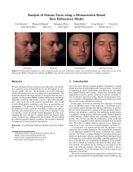
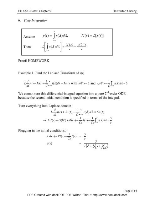
EE 422G Notes: Chapter 5Instructor: Cheung6. Time IntegrationtAssume y( t)= ∫ x(λ ) dλ,X ( s)= L[x(t)]−∞t⎡ ⎤Then L ⎢ x() d ⎥⎣ −∫ λ λ∞ ⎦X ( s)= +sy (0s−)Proof: HOMEWORKExample 1: Find the Laplace Transform of i (t)dLdt1 t−− 1 0i( t)+ Ri(t)+ i() d = 5u(t)C∫ λ λ−∞with i ( 0 ) = 0 and ∫ −v c( 0 ) = i(λ)dλ= 0C −∞We cannot turn this differential-integral equation into a pure 2 nd -order ODEbecause the second initial condition is specified in terms of the integral.Turn everything into Laplace domaind1 tL i( t)+ Ri(t)+ i() d = 5u(t)dtC∫ λ λ−∞1 1 0−5→ LsI(s)− Li(0) + RI(s)+ I ( s)+ i() d =Cs Cs∫ − λ λ−∞sPlugging in the initial conditions:1LsI(s)+ RI(s)+ I ( s)CsI(s)==5s2( + R s + 1 )L s5LLCPage 5-14PDF Created with deskPDF PDF Writer - Trial :: http://www.docudesk.com

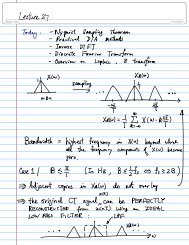
EE 422G Notes: Chapter 5Instructor: Cheung1Example 2 : Find the inverse Laplace Transform of X ( s)= + 1( s + α)nWe first look at the Laplace transform of X ( s)= 1s nas the α is just a simple+ 1frequency shifting (see property 2).Observe that:X ( s)= 1s⇔ x(t)= u(t)X ( s)= 12s⇔t−x(t)= ∫ u(λ)dλ= tu(t),x(0) = 0−∞2t t−X ( s)= 13 ⇔ x(t)= ∫ tu(λ)dλ= u(t),x(0) = 0s−∞2MM Mn−1nt ttX ( s)= 1n+1 ⇔ x(t)= ∫ u(λ)dλ= u(t),s−∞( n −1)!n!x(0Putting back the frequency shift, we havent −αtx( t)= e u(t)n!7. Initial Value Theoremx(t)= L⇒ x(0+−1[ X ( s)]) =lim sX ( s)s→∞−) = 0This theorem says the behavior of x at t=0 (transient state) can be evaluated bytaking s → ∞ for the Laplace transform sX(s) .Intuitively, it makes sense to be able to recover the initial condition directly fromthe Laplace transform.Proof:From the time differentiation property, we know− ⎡ dsX ( s)− x(0) = L⎢⎣ dt= ∫ ∞ d0dtTake the limit s → ∞ on both side⎤x(t)⎥⎦x(t)e− stdtPage 5-15PDF Created with deskPDF PDF Writer - Trial :: http://www.docudesk.com

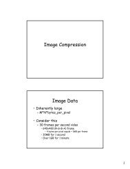
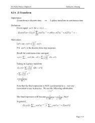
EE 422G Notes: Chapter 5Instructor: Cheunglims→∞−sX ( s)− x(0)==lims→∞∫0∞ddtx(t)estLet’s consider the behavior of e − as s → ∞real part as it will dominate the behavior of the functions.1−stdt∞ d−st∫ x(t)lims→∞e dt0dt. Again it is sufficient to consider they0.90.80.70.60.5as s goes to ∞.0.4e -t0.30.2e -5t e -2t0.1e -10t00 1 2 3 4 5xlim−→∞e sts⎧ 1 t = 0= ⎨⎩0otherwiseNote that this is not a delta function! Maindifference: unless f(t) is ∞ at t=0.∫f ( t) lims→∞e−st⎧0dt = ⎨⎩αf ( t)finite at t = 0f ( t)= αδ ( t)+ KddtCase 1: x(t)is finite at t=0.ddtSince x(t)ddtlims → ∞sX ( s)= x(0+−is finite at t=0, x (t)is continuous at t=0 so x (0 ) = x(0)lim+ −Case 2: x( t)= ( x(0) − x(0)) δ ( t)+ ...Proof complete.s → ∞sX ( s)= x(0− + − +lims → ∞sX ( s)− x(0) = x(0) − x(0) = x(0)Example 1: A demonstration where x(0) is obvious−αtx( t)= e cosω0tu(t)0It is evident: x 0) = e− cosω⋅ 0 = 1( 0Using Laplace transforms + αX ( s)= L[x(t)]=2( s + α ) + ω20−+)). HencePage 5-16PDF Created with deskPDF PDF Writer - Trial :: http://www.docudesk.com

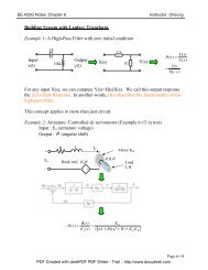
EE 422G Notes: Chapter 5Instructor: CheungExample 2: Find the final value of x(t) given1X ( s)= s − 3sUsing the Final Value Theorem: x( ∞)= lims 0= 0→s − 33tTaking the inverse Laplace transform will get x(t)= e u(t)which blows up!!!What’s wrong here?The ROC of sX(s) does not include the imaginary axis!!!8. Time ConvolutionAssume L x ( t)]= X ( ) and L x ( t)]= X ( )Note: You may be more familiar with this form of convolution:∞( ∫ 1 2−∞y t)= x ( λ)x ( t − λ)dλx ∞1< ⇒ y(t)= ∫ x1 ( λ)x2(t − λ)d λ0tx ( t − λ)= 0 ∀λ> t2 ⇒ y(t)= ∫ x1 ( λ)x2(t − λ)d λ0if ( t)= 0 ∀t0ifTherefore,ty(t)= ∫ x ( λ)x ( t − λ dλ01 2)Now, we can proceed with the calculation of the integral:L[t∫0∞∫[∫x1 ( λ ) x2(t − λ)dλ]= x1(λ)x2(t − λ)dλ]eReplace t with ∞,[1 1s=t0 0∞ ∞∫ ∫Exchange order of int., = ∫ x λ)∫λ[2 2stTheir convolution can be defined as y( t)≡ ∫ x ( λ ) x ( t − λ dλ1 2)0[1 2sand its Laplace transform is L y(t)]= X ( s)X ( )λλ−stdt−st[ x1 ( ) x2(t − ) d ] e dt0 0∞ ∞−st1( x2(t − λ)e dt dλ0 0Page 5-18PDF Created with deskPDF PDF Writer - Trial :: http://www.docudesk.com

EE 422G Notes: Chapter 5Instructor: Cheung−s(τ + λ)Substitute τ = t − λ , = ∫ x1 ( λ)∫ x2(τ ) e dt dλ[ ]∞0∞−λ−sλx ( τ ) = 0∀τ ∈ −λ0 =2∫ x λ)e ∫=∞∞−sτ1( x2(τ ) e dt dλ0 0∞∫0x ( λ)e211∞∫= X ( s)0= X ( s)X−sλx ( λ)e21( s)X ( s)dλ2−sλThis is a partial list of the Laplace Transforms of common functions. Rememberthem!!There are more transform pairs from Table 5-3 in the book (page 220). You do notneed to remember them but you should be able to derive them. I will assign someof them as homework problems.dλPage 5-19PDF Created with deskPDF PDF Writer - Trial :: http://www.docudesk.com