Z-transform and its inverse

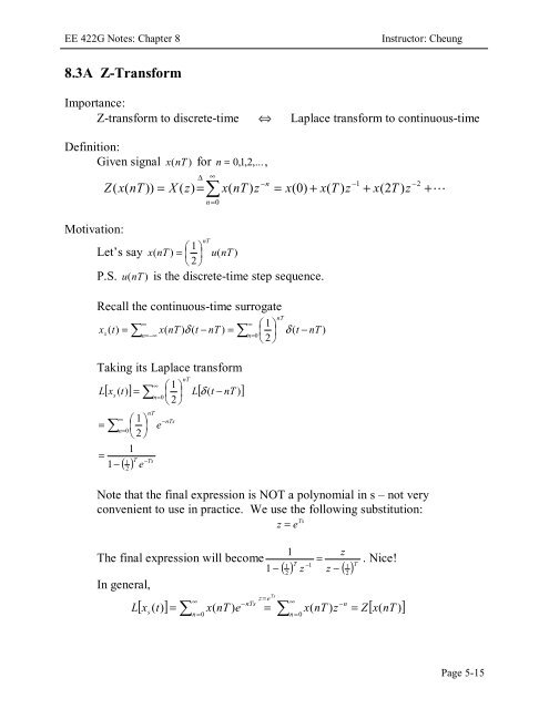
EE 422G Notes: Chapter 8Instructor: Cheung8.3A Z-TransformImportance:Z-transform to discrete-time ⇔ Laplace transform to continuous-timeDefinition:Given signal x (nT ) for n = 0,1,2 ,...,∆∞∑−n−1Z( x(nT )) = X ( z)= x(nT ) z = x(0)+ x(T ) z + x(2T) zn=0−2+LMotivation:nT⎛ 1 ⎞Let’s say x( nT ) = ⎜ ⎟ u(nT )⎝ 2 ⎠P.S. u (nT ) is the discrete-time step sequence.Recall the continuous-time surrogate∞∞ ⎛ 1 ⎞xs( t)= ∑ x(nT ) δ ( t − nT ) ==−∞ ∑ ⎜ ⎟ δ ( t − nT )nn=0⎝ 2 ⎠Taking its Laplace transformL=∞[ xs( t)] = ∑ ⎜ ⎟ L[ δ ( t − nT )]∑∞=1−n=0⎛ 1 ⎞⎜ ⎟⎝ 2 ⎠1nT1 T −Ts( ) e2n=0e⎛ 1 ⎞⎝ 2 ⎠−nTsnTNote that the final expression is NOT a polynomial in s – not veryconvenient to use in practice. We use the following substitution:Tsz = eThe final expression will become1 −In general,LnTz1( ) T −11z − ( ) T21=z2. Nice!∞z = e−nTs∞−n[ x ( t)] = x(nT ) e = x(nT ) z = Z[ x(nT )]s∑n=0Ts∑n=0Page 5-15

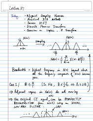
EE 422G Notes: Chapter 8Instructor: CheungConsequences:1. Left half s-plane → Inside the unit circle in z-planeRight half s-plane → Outside of the unit circle in z-planeImaginary axis in s-plane → Unit circle in z-plane2. ROC in S-plane {s: Re(s) > p} → ROC in Z-plane {z: |z| > r}3. H(s) is BIBO stable if all poles are on the left half plane →H(z) is BIBO stable if all poles are inside the unit circle (more later)4. Fourier Transform in S-plane is evaluated along jω-axis →Fourier Transform in Z-plane is evaluated along the unit circle⇒ X s (e jωT j( ωT+ 2nπ)) must be the same as X s( e ) , i.e. integral number of full2nπrotation. As j ( ω T + 2nπ) = j(ω + ) T , the Fourier transform is a periodicT2πfunction in ω with period = = ωs. We have seen this before!T-ω hX(jω)↓ after samplingω hX s (jω)-ω s -ω h -ω s -ω s +ω h -ω h ω s -ω hω hω sω s +ω h2ω sPage 5-17

EE 422G Notes: Chapter 8Instructor: CheungExamples of Z-transformsExample 8-4: z-transform of unit pulse δ (n):⎧1n = 0⎫∆x( nT)= ⎨⎬=δ ( n)⎩0n ≠ 0⎭X ( z)= 1+0⋅z−1+ L = 1Example 8-5 z-Transform of unit step sequence u(nT):⎧1n ≥ 0x ( nT ) = ⎨⎩0n < 0X ( z)= 1 + z1=1 − z−1−1+ z−2+ Lwith ROC ={z: |z| > 1}Typically, we write the Z-transform in terms of z -1 rather than z as casualsequences contain only the negative powers of z.Poles and Zeros in Z-transform:1X ( z)= has a pole at z = c and a zero at z = 0−11−cz−11−czX ( z)= has a zero at z = c and a pole at z = ∞−1zProperties Time Domain Z Transform1 Linearity a1x1( nT ) + a2x2(nT ) a1X1( z)+ a2X2(z)n2 Multiply by a a n x(nT )⎛ z ⎞X ⎜ ⎟⎝ a ⎠3 Time Delay x ( nT − mT ) u(nT − mT ), m > 0 z m X (z)4 Multiply by n nx (nT )d− z X (z)dz5 Initial Value Theorem x( 0) = limz→∞X ( z)6 Final Value Theorem x(∞ ) = lim−1(1 − z ) X ( )7 Time Convolution ∑ ∞ m=0z→1 zx ( mT ) y(nT − mT ) X ( z)Y ( z)Page 5-18

EE 422G Notes: Chapter 8Instructor: CheungnMultiply by aZ−nn∞ n−n∞ ⎛ z ⎞ ⎛ z ⎞[ a x(nT )] = ∑ a x(nT ) z = ∑ x(nT ) ⎜ ⎟ = X ⎜ ⎟ ⎠n=0n=0⎝ a ⎠−αnTEx: Find the Z-transform of y( nT ) = e u(nT )−αT nRewrite y( nT ) ( e ) u(nT )Multiply by ndX ( z)− z = −zdz= −z⎝ a1Z ( ,−1−z11==−1 −1−( z ) 1−e z−αTe= . Given [ u nT )] =1Z[ y nT )] 1(αT−d−1−2−3( x(0)+ x(T ) z + x(2T) z + x(3T) z + ...)dz−2−3−4( − x(T ) z − 2x(2T) z − 3x(3T) z − ...)= 0⋅x(0)+ 1⋅x(T ) z−1+ 2⋅x(2T) zEx. Find the Z-transform of y ( nT ) = nTu(nT )T1−z−2+ 3⋅x(3T) zd Tdz 1−z−3+ ... = ZTz(1 − zSince Z [ Tu( nT )] = , Z [ nTu( nT )] = −z=−1−1−12Initial Value TheoremX ( z)= x(0)+ x(1)z−1−1)( nx(nT ))+L. Having z goes to ∞ kills every term except the first.Final Value Theorem−1Final value x(∞ ) = lim(1 − z ) X ( z)if X (z)does not have any poles on or outsidez→1the unit circle, except possibly a simple pole at z = 1.A formal proof is beyond the scope but here is an informal proof:(1 − zz = 1−1) X ( z)= x(0)+ [ x(T ) − x(0)]z+ [ x(2T) − x(T )] z= x(0)+ x(T ) − x(0)+ x(2T) − x(T ) + x(3T) − x(2T) = x(∞)−1−2+ [ x(3T) − x(2T)] z−3+ ...Page 5-19

EE 422G Notes: Chapter 8Instructor: CheungCommonly used Z-transform pairs8.3B Inverse Z-TransformTwo Basic Methods:−11. Express X(z) into “Definition Form” X ( z)= x(0)+ x(1)z + L−1−2−3−4ex. X ( z)= 1+2z− 5z− 2z+ zThis implies x ( 0) = 1, x(T ) = 2, x(2T) = −5,x(3T) = −2,x(4T) = 1,and zero otherwise.1ex. Long division X ( z)=−1(1 − az )1−az−11+az) 11−azazaz−1−1−1−12+ a z− a zaM−22 −2z2 −2+ ...n⇒ x( nT ) = a u(nT )Page 5-20

EE 422G Notes: Chapter 8Instructor: Cheung2. Express X(z) into partial-fraction fromNN−kβk−1Expand X ( z)= ∑α kz + ∑ , all in terms of z− mk(1 − a z1 )k = 0 k=0↑↑each term has an inverse transformkImportant: before doing partial-fraction expansion, make sure the z-−1transform is in proper rational function ofz !Example 8.92zX z)==( z −1)(z − 0.2) (1 − z1)(1 − 0.2z(−1−1)Solution :X( z)== +−1−1−1− 1(1 − z1)(1 − 0.2z)A1−zB1−0.2zHeaviside’s Expansion Method:(1)−11(1 − z ) X ( z)=−11−0.2z1 B ⋅ 0= A + ⇒1−0.2 1−0.2−1B(1− z )= A + ⇒−11−0.2z1A = = 1.250.8z=1−1−1A(1− 0.2z) B ⋅(1− 0.2z(2) ( 1−0.2z) X ( z)=+−1−11−z 1−0.2z11−zA(1− 0.2z=−1−z−11−1)+ B1 − 0.2 z−10 ( 0.2)⇒ = z =−1)B = −0.251.25 − 0.25X ( z)= + ⇒ x(nT ) = 1.25 − 0.25(0.2)− 1 −11−z 1−0.2znPage 5-21