Analysis of Human Faces using a Measurement-Based Skin ...

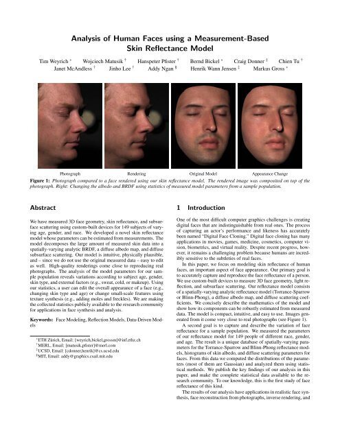
Analysis of Human Faces using a Measurement-BasedSkin Reflectance ModelTim Weyrich ∗ Wojciech Matusik † Hanspeter Pfister † Bernd Bickel ∗ Craig Donner ‡ Chien Tu †Janet McAndless † Jinho Lee † Addy Ngan § Henrik Wann Jensen ‡ Markus Gross ∗Photograph Rendering Original Model Appearance ChangeFigure 1: Photograph compared to a face rendered using our skin reflectance model. The rendered image was composited on top of thephotograph. Right: Changing the albedo and BRDF using statistics of measured model parameters from a sample population.AbstractWe have measured 3D face geometry, skin reflectance, and subsurfacescattering using custom-built devices for 149 subjects of varyingage, gender, and race. We developed a novel skin reflectancemodel whose parameters can be estimated from measurements. Themodel decomposes the large amount of measured skin data into aspatially-varying analytic BRDF, a diffuse albedo map, and diffusesubsurface scattering. Our model is intuitive, physically plausible,and – since we do not use the original measured data – easy to editas well. High-quality renderings come close to reproducing realphotographs. The analysis of the model parameters for our samplepopulation reveals variations according to subject age, gender,skin type, and external factors (e.g., sweat, cold, or makeup). Usingour statistics, a user can edit the overall appearance of a face (e.g.,changing skin type and age) or change small-scale features usingtexture synthesis (e.g., adding moles and freckles). We are makingthe collected statistics publicly available to the research communityfor applications in face synthesis and analysis.Keywords: Face Modeling, Reflection Models, Data-Driven Models∗ ETH Zürich, Email: [weyrich,bickel,grossm]@inf.ethz.ch† MERL, Email: [matusik,pfister]@merl.com‡ UCSD, Email: [cdonner,henrik]@cs.ucsd.edu§ MIT, Email: addy@graphics.csail.mit.edu1 IntroductionOne of the most difficult computer graphics challenges is creatingdigital faces that are indistinguishable from real ones. The processof capturing an actor’s performance and likeness has accuratelybeen named “Digital Face Cloning.” Digital face cloning has manyapplications in movies, games, medicine, cosmetics, computer vision,biometrics, and virtual reality. Despite recent progress, however,it remains a challenging problem because humans are incrediblysensitive to the subtleties of real faces.In this paper, we focus on modeling skin reflectance of humanfaces, an important aspect of face appearance. Our primary goal isto accurately capture and reproduce the face reflectance of a person.We use custom-built devices to measure 3D face geometry, light reflection,and subsurface scattering. Our reflectance model consistsof a spatially-varying analytic reflectance model (Torrance-Sparrowor Blinn-Phong), a diffuse albedo map, and diffuse scattering coefficients.We concisely describe the mathematics of the model andshow how its components can be robustly estimated from measureddata. The model is compact, intuitive, and easy to use. Images generatedfrom it come very close to real photographs (see Figure 1).A second goal is to capture and describe the variation of facereflectance for a sample population. We measured the parametersof our reflectance model for 149 people of different race, gender,and age. The result is a unique database of spatially-varying parametersfor the Torrance-Sparrow and Blinn-Phong reflectance models,histograms of skin albedo, and diffuse scattering parameters forfaces. From this data we computed the distributions of the parameters(most of them are Gaussian) and analyzed them using statisticalmethods. We publish the key findings of our analysis in thispaper, and make the complete statistical data available to the researchcommunity. To our knowledge, this is the first study of facereflectance of this kind.The results of our analysis have applications in realistic face synthesis,face reconstruction from photographs, inverse rendering, and

3 Skin Reflectance ModelThe BSSRDF is a function S(x i ,ω i ,x o ,ω o ), where ω i is the directionof the incident illumination at point x i , and ω o is the observationdirection of radiance emitted at point x o . The outgoing radianceL(x o ,ω o ) at a surface point x o in direction ω o can be computed byintegrating the contribution of incoming radiance L(x i ,ω i ) for allincident directions Ω over the surface A:∫ ∫L(x o ,ω o ) = S(x i ,ω i ,x o ,ω o )L(x i ,ω i )(N · ω i )dω i dA(x i ). (1)A ΩWe will use the notation dx i for (N · ω i )dA(x i ).We separate this integral into a specular BRDF term and a diffusesubsurface scattering term:L(x o ,ω o ) = L specular (x o ,ω o ) + L di f f use (x o ,ω o ), (2)with:∫L specular (x o ,ω o ) = f s (x o ,ω o ,ω i )L(x o ,ω o )(N · ω i )dω i , (3)Ω∫ ∫L di f f use (x o ,ω o ) = S d (x i ,ω i ,x o ,ω o )L(x i ,ω i )dω i dx i . (4)A ΩS d (x i ,ω i ,x o ,ω o ) is called the diffuse BSSRDF and f s (x o ,ω o ,ω i ) isa surface BRDF. As observed in [Jensen and Buhler 2002], multiplescattering dominates in the case of skin and can be modeled as apurely diffuse subsurface scattering term and a specular term thatignores single scattering (see Figure 2).w ix iSpecular Reflection (BRDF) f sw ix ow oModulation Texture MHomogeneous SubsurfaceScattering RFigure 2: Spatially-varying skin reflectance can be explained by aspecular BRDF f s at the air-oil interface, and a diffuse reflectancecomponent due to subsurface scattering. We model the diffuse reflectancewith a spatially-varying modulation texture M and a homogeneoussubsurface scattering component R d .The diffuse BSSRDF S d is very difficult to acquire directly.Consequently, it is often decomposed into a product of lowerdimensionalfunctions. A commonly used decomposition for S dis:S d (x i ,ω i ,x o ,ω o ) ≈ 1 π f i(x i ,ω i )R d (x i ,x o ) f o (x o ,ω o ). (5)Here R d (x i ,x o ) describes the diffuse subsurface reflectance of lightentering at point x i and exiting at point x o . The diffuse surfacereflectance/transmittance functions f i (x i ,ω i ) and f o (x o ,ω o ) furtherattenuate the light at the entrance and exit points based on the incomingand outgoing light directions, respectively.The complete formula for our skin model is:∫L(x o ,ω o ) = f s (x o ,ω o ,ω i )L(x o ,ω i )(N · ω i )dω i (6)Ω∫ ∫+ F ti R d (||x o − x i ||)M(x o )F to L(x i ,ω i )dω i dx i .A ΩLike Jensen et al. [2001; 2002], we assume that skin is mostlysmooth and use transmissive Fresnel functions F ti = F t (x i ,ω i ) andF to = F t (x o ,ω o ). We use η ≅ 1.38 as the relative index of refractionbetween skin and air for the Fresnel terms [Tuchin 2000].We model the diffuse reflectance using a homogeneous subsurfacereflectance term R d (||x o − x i ||) and a spatially-varying modulationtexture M(x o ) [Fuchs et al. 2005a]. Intuitively, this modulationtexture represents a spatially-varying absorptive film of zerothickness on top of homogeneously scattering material (see Figure2). To model homogeneous subsurface scattering we use thedipole diffusion approximation by Jensen et al. [2001]. It simplifiesR d (x i ,x o ) to a rotationally-symmetric function R d (||x o − x i ||),or R d (r) with radius r. Jensen and Buhler [Jensen and Buhler 2002]develop fast rendering methods for this approximation, and Donnerand Jensen [2005] extend it to a multipole approximation for multiplelayers of translucent materials.Our formulation in Equation (6) was motivated by the skin modelshown in Figure 2. Goesele et al. [2004] assume f i (x i ,ω i ) andf o (x o ,ω o ) to be constant. To model inhomogeneous translucentmaterials, they exhaustively measure R d (x i ,x o ) and tabulate the results.In follow-up work [Fuchs et al. 2005a] they fit a sum of Gaussiansto the tabulated values of R d (x i ,x o ) to model anisotropic scattering.However, acquiring R d (x i ,x o ) directly requires a substantialexperimental setup (controlled laser illumination from different angles)that is not applicable for human faces.Donner and Jensen [2005] use spatially-varying diffuse transmissionfunctions ρ dt (x i ,ω i ) = 1 − ∫ Ω f s(x i ,ω i ,ω o )(ω o · n)dω o(similarly for ρ dt (x o ,ω o )). They integrate a BRDF at the surfaceover the hemisphere of directions and tabulate the results to obtainthe diffuse transmission functions. To capture materials with homogeneoussubsurface scattering and complex surface mesostructure(so-called quasi-homogeneous materials), Tong et al. [2005] measureand tabulate a spatially-varying exit function f o (x o ,ω o ) and auniform entrance function f i (ω i ). We now give an overview of howwe measure and estimate the parameters of our model.4 Parameter Estimation OverviewA block diagram of our processing pipeline is shown in Figure 3.We first capture the 3D geometry of the face using a commercial 3D3D SurfaceScanSpecularReflectanceBRDF FitSpatially-VaryingSpecular BRDFReflectanceMeasurementsNormal Map andDiffuse ReflectanceEstimationDiffuse AlbedoDiffuse SubsurfaceScatteringSubsurfaceScansDipole Model Fitsigma a / sigma' sFigure 3: A block diagram of our data processing pipeline. Blocksin grey are the parameters of our skin reflectance model.face scanner. Then we measure the total skin reflectance L(x o ,ω o )in a calibrated face-scanning dome by taking photographs from differentviewpoints under varying illumination. We refine the geometryand compute a high-resolution face mesh and a normal mapusing photometric stereo methods. To map between 3D face spaceand 2D (u,v) space we use the conformal parameterization of Shefferet al. [2005]. The data is densely interpolated using push-pullinterpolation into texture maps of 2048 × 2048 resolution.

The reflectance measurements are registered to the 3D geometryand combined into lumitexels [Lensch et al. 2001]. Each lumitexelstores samples of the skin BRDF f r (x o ,ω i ,ω o ). We estimate thediffuse reflectance α(x o ) of f r using a stable minimum of lumitexelsamples. Note that this diffuse reflectance encompasses theeffects of the diffuse subsurface scattering R d (r) and the modulationtexture M(x o ). We store α(x o ) in a diffuse albedo map and subtractit from f r (x o ,ω i ,ω o ). To the remaining specular reflectancef s (x o ,ω i ,ω o ) we fit the analytic BRDF function.The diffuse subsurface reflectance R d (r) and the modulation textureM(x o ) cannot be measured directly on human subjects. Instead,we measure their combined effect R(r) at a few locations in the faceusing a special contact device. To our measurements R(r) we fit theanalytic dipole approximation of Jensen et al. [2001] and store thereduced scattering coefficient σ ′ s and the absorption coefficient σ a .Similar to Donner and Jensen [2005] we derive that:R d (r)M(x o ) = R(r) α(x o)α avg, (7)where α avg is the average albedo. We use the albedo map α(x o ),the average of all albedo map values α avg , and the dipole approximationfor R(r) to compute R d (r)M(x o ) in Equation (6).In summary, the parameters for each face are the spatiallyvaryingcoefficients of the specular BRDF f s , an albedo map withdiffuse reflectance values α(x o ), and the values for σ ′ s and σ a . Section6 describes how this data is used for rendering. We now describeeach of these measurement and processing steps in more detail.5 Measurement SystemFigure 4 shows a photograph of our face-scanning dome. The sub-Figure 5: Facial detail shown in closeups. Left: Measured geometrybefore correction. Middle: Corrected high-quality geometry.No normal map was used; the surface detail is due to the actualgeometry of the model. Right: Comparison photo.close their eyes. We report more details about the system and itscalibration procedure in [Weyrich et al. 2006].A commercial face-scanning system from 3QTech(www.3dmd.com) is placed behind openings of the dome.Using two structured light projectors and four cameras, it capturesthe complete 3D face geometry in less than one second. The outputmesh contains about 40,000 triangles and resolves features assmall as 1 mm. We clean the output mesh by manually croppingnon-facial areas and fixing non-manifold issues and degenerate triangles.The cleaned mesh is refined using Loop-subdivision [Loop1987] to obtain a high-resolution mesh with about 700,000 to900,000 vertices. The subdivision implicitly removes noise.Next, we compute a lumitexel [Lensch et al. 2001] at each vertexfrom the image reflectance samples. The lumitexel radiance valuesL(x o ,ω o ) are normalized by the irradiance E(x o ,ω i ) to obtainBRDF sample values:f r (x o ,ω i ,ω o ) = L(x o,ω o )E(x o ,ω i ) = L(x o ,ω o )∫Ω L(ω i)(ω i · n)dω i. (8)We calibrate the radiance L(ω i ) of each light source using a whiteideal diffuse reflector (Fluorilon) and explicitly model the beamspread by a bi-variate 2 nd degree polynomial [Weyrich et al. 2006].We use shadow mapping to determine the visibility of lumitexelsamples for each light source and camera. On average, a lumitexelcontains about 900 BRDF samples per color channel, with manylumitexels having up to 1,200 samples. The numbers vary dependingon the lumitexel visibility. All processing is performed on RGBdata except where noted otherwise.5.1 Geometry ProcessingFigure 4: The face-scanning dome consists of 16 digital cameras,150 LED light sources, and a commercial 3D face-scanning system.ject sits in a chair with a headrest to keep the head still during thecapture process. The chair is surrounded by 16 cameras and 150LED light sources that are mounted on a geodesic dome. The systemsequentially turns on each light while simultaneously capturingimages with all 16 cameras. We capture high-dynamic range (HDR)images [Debevec and Malik 1997] by immediately repeating thecapture sequence with two different exposure settings. The completesequence takes about 25 seconds for the two passes throughall 150 light sources (limited by the frame rate of the cameras). Tominimize the risk of light-induced seizures we ask all subjects toWe estimate normals at each lumitexel from the reflectance data usingphotometric stereo [Barsky and Petrou 2001]. We compute anormal map for each of the camera views. Using the method byNehab et al. [2005] we correct low-frequency bias of the normals.For each camera, we also compute the cosine between it and eachnormal and store the result as a blending weight in a texture. Tocompute the final diffuse normal map, we average all normals ateach vertex weighted by their blending weights. To avoid seamsat visibility boundaries between cameras, we slightly smooth theblending texture and the diffuse normal map using a Gaussian filter.Finally, we compute the high-resolution geometry by applyingthe method of Nehab et al. a second time. Figure 5 compares themeasured 3QTech geometry to the final high-resolution mesh.Figure 6 (a) shows a rendering of a face using the Torrance-Sparrow BRDF model and the diffuse normal map. The renderingdoes not accurately reproduce the specular highlights that are visiblein the input photo in Figure 6 (d). For example, compare thedetailed highlights on the cheeks in (d) with the blurred highlightin (a). These highlights are due to micro-geometry, such as poresor very fine wrinkles, which is not accurately captured in the facegeometry or diffuse normal map.

Figure 6: Torrance-Sparrow model and (from left to right) (a) onlydiffuse normal map; (b) one diffuse and one global micro-normalmap for specular reflection; (c) one diffuse and per-view micronormalmaps; (d) input photograph. Method (c) most accuratelyreproduces the specular highlights of the input image.To improve the result, we use micro-normals to render the specularcomponent. Debevec et al. [Debevec et al. 2000] used micronormalsfor a Torrance-Sparrow model on their specular term. Theyestimated improved normals using a specular reflection image obtainedusing cross-polarized lighting. For each camera viewpoint,we choose the sample with maximum value in each lumitexel. Thehalf-way vector between the view direction and the sample’s lightsource direction is the micro-normal for this view. We either storethese normals in per-camera micro-normal maps, or generate a singlemicro-normal map using the blending weights from before. Figures6 (b) and (c) show renderings with single or per-view micronormalmaps, respectively. Figure 6 (b) is better than (a), but onlyFigure 6 (c) accurately reproduces the highlights of the input image.The results in this paper were computed using per-view micronormals.For between-camera views and animations we interpolatethe micro-normals with angular interpolation [Debevec et al. 1996].5.2 Diffuse Albedo EstimationWe estimate the total diffuse reflectance α at each surface pointfrom the lumitexel data. We assume that we observe pure diffusereflectance at each lumitexel for at least some of the observationangles. The total diffuse reflectance is the maximum value that isless than or equal to the minimum of all the BRDF samples f r . Wecompute α as the minimum ratio between f r and the unit diffusionreflectance:α(x o ) = min iπ f r (x o ,ω o ,ω i )F t (x o ,ω i )F t (x o ,ω o ) . (9)Note that we divide f r by the transmissive Fresnel coefficients. Inorder to reduce outliers and the influence of motion artifacts, we determinea stable minimum by penalizing grazing observations anddiscarding the k smallest values. The α values for each surfacepoint are re-parameterized, interpolated, and stored as the diffusealbedo map.5.3 BRDF FitThe specular reflection is computed at each lumitexel by subtractingthe total diffuse reflectance:f s (x o ,ω o ,ω i ) = f r (x o ,ω o ,ω i ) − α(x o)π F t(x o ,ω i )F t (x o ,ω o ). (10)Highlights on dielectric materials like skin are of the same coloras the light source (white, in our case). Consequently, we convertthe specular reflectance to grey scale to increase the stability of theBRDF fit. Unlike previous work [Marschner et al. 1999; Lenschet al. 2001; Fuchs et al. 2005b] we do not need to cluster reflectancedata because our acquisition system collects enough samples for aspatially-varying BRDF fit at each vertex. The data for lumitexelswith a badly conditioned fit is interpolated during creation of theBRDF coefficient texture.We fit the Blinn-Phong [Blinn 1977] and Torrance-Sparrow [Torranceand Sparrow 1967] isotropic BRDF models to the data. TheBlinn-Phong model is the most widely used analytic reflectancemodel due to its simplicity:f sBP = ρ sn + 22π cosn δ. (11)Here δ is the vector between the normal N and the half-way vectorH, ρ s is the scaling coefficient, and n is the specular exponent. Thefactor (n+2)/2π is for energy normalization so that the cosine lobealways integrates to one. This assures that 100% of the incidentenergy is reflected for ρ s = 1.We also use the physically-based Torrance-Sparrow model:with:1 DGf sT S = ρ sπ (N · ω i )(N · ω o ) F r(ω o · H), (12)G = min{1, 2(N · H)(N · ω o), 2(N · H)(N · ω i)}, (13)(ω o · H) (ω o · H)1D =m 2 cos 4 δ exp−[(tanδ)/m]2 .G is the geometry term, D is the Beckmann micro-facet distribution,and F r is the reflective Fresnel term. The free variables are thescaling coefficient ρ s and the roughness parameter m.For the fit we use the fitting procedure by Ngan et al. [2005]. Theobjective function of the optimization is the mean squared errorbetween the measured BRDF f s and the target model f sM (eitherf sBP or f sT S ) with parameter vector p:√∑w[ f s (ω i ,ω o )cosθ i − f sM (ω i ,ω o ;p)cosθ i ]E(p) =2. (14)∑wThe sum is over the non-empty samples of the lumitexel, and θ i isthe elevation angle of incident direction. The weight w is a correctionterm that allows us to ignore data with ω i or ω o greater than80 ◦ . Measurements close to extreme grazing angles are generallyunreliable due to imprecisions in the registration between 3D geometryand camera images. We apply constrained nonlinear optimizationbased on sequential quadratic programming over the specularlobe parameters to minimize the error metric.To assess the quality of our fit, we compare renderings from cameraviewpoints to the actual photographs. The camera and lightsource calibration data were used to produce identical conditionsin the renderings. Figure 7 shows a comparison of the originaland synthesized images with the same illumination and differentBRDF models. The spatially-varying Blinn-Phong model (c) overestimatesthe specular component and does not match the photographas closely as the spatially-varying Torrance-Sparrow model(b). Nevertheless, it produces more accurate results compared tothe spatially uniform Torrance-Sparrow BRDF (d).Another popular choice for BRDF fitting is the Lafortunemodel [Lafortune et al. 1997] because it models off-specular reflectionswhile still being computationally simple. Because thenon-linear Lafortune model has more parameters than the Torrance-Sparrow and Blinn-Phong models, fitting of the model becomesmore demanding, even for a single-lobe approximation. A realisticemployment of the Lafortune model would use at least three lobes.This fit has been reported by [Ngan et al. 2005] to be very unstablecompared to other reflectance models. In addition, [Lawrence et al.2004] explain that “Often, a nonlinear optimizer has difficulty fittingmore than two lobes of a Lafortune model without careful userintervention.” Given the high quality that we could achieve with theTorrance-Sparrow model, we decided not to further investigate theLafortune model.

(a) (b) (c) (d)Figure 7: (a) Input photograph compared to our face model with (b) spatially-varying Torrance-Sparrow; (c) spatially-varying Blinn-Phong;and (d) uniform Torrance-Sparrow BRDF models.5.4 Measuring TranslucencyOur subsurface measurement device is an image-based version ofa fiber optic spectrometer with a linear array of optical fiber detectors[Nickell et al. 2000] (see Figure 8). Similar, more sophisticatedFigure 9: Left: The sensor head placed on a face. Top: Sensor fiberlayout. The source fiber is denoted by a cross. Bottom: An HDRimage of the detector fibers displayed with three different exposurevalues.Figure 8: Left: A picture of the sensor head with linear fiber array.The source fiber is lit. Right: The fiber array leads to a camera ina light-proof box. The box is cooled to minimize imaging sensornoise.devices called Laser Doppler Flowmetry (LDF) probes are usedto measure micro-circulatory blood flow and diffuse reflectance inskin [Larsson et al. 2003]. The advantage of our device over LDF orthe measurement procedure in [Jensen et al. 2001] is that it can besafely used in faces. Light from a white LED is coupled to a sourcefiber. The alignment of the fibers is linear to minimize sensor size.A sensor head holds the source fiber and 28 detection fibers. A digitalcamera records the light collected by the detector fibers. Thecamera and detector fibers are encased in a light-proof box with aircooling to minimize imager noise. We capture 23 images bracketedby 2/3 f-stops to compute an HDR image of the detector fibers. Thetotal acquisition time is about 88 seconds.Figure 9 shows the sensor head placed on a face. We have chosento measure three points where the sensor head can be placed reliably:forehead, cheek, and below the chin. For hygienic reasons wedo not measure lips. We found that pressure variations on the skincaused by the mechanical movement of the sensor head influencethe results. To maintain constant pressure between skin and sensorhead we attached a silicone membrane connected to a suctionpump. This greatly improves the repeatability of the measurements.For more details on the subsurface device and calibration proceduresee [Weyrich et al. 2006].Previous work in diffuse reflectometry [Nickell et al. 2000] suggeststhat some areas of the human body exhibit anisotropic subsurfacescattering (e.g., the abdomen). We measured two-dimensionalsubsurface scattering on the abdomen, cheek, and forehead for afew subjects. We verified the presence of significant anisotropy inthe abdominal region (see Figure 10). However, the plots showFigure 10: Subsurface scattering curves for abdomen, cheek, andforehead measured along 16 1D profiles.that the diffuse subsurface scattering of facial skin can be well approximatedwith an isotropic scattering model. Consequently, wemeasure only a one-dimensional profile and assume rotational symmetry.We fit the analytic BSSRDF model of Jensen et al. [2001] tothe data points of each subsurface measurement, providing us withthe reduced scattering coefficient σ ′ s and absorption coefficient σ a .From the measured σ a and σ ′ s data we can derive the effective transportcoefficient:σ tr = √ 3σ a (σ a + σ ′ s) ≈ 1/l d . (15)l d is the diffuse mean free path of photons (mm) and provides ameasure of skin translucency.Table 1 shows the mean and variance of σ tr for a sample populationof various people (see Section 7). The measurement points oncheek and forehead are quite similar in translucency. The measurementpoint on the neck underneath the chin shows a rather different

σ tr Cheek Forehead Neck(mm −1 ) Mean Var. Mean Var. Mean Var.red 0.5572 0.1727 0.5443 0.0756 0.6911 0.2351green 0.9751 0.2089 0.9831 0.1696 1.2488 0.3686blue 1.5494 0.1881 1.5499 0.2607 1.9159 0.4230Table 1: Mean and variance of σ tr in our dataset.mean, but also higher variance. This is probably due to measurementnoise, as the sensor head is hard to place there.Figure 11 shows closeups of the subjects with minimum[1.0904,0.6376,0.6035] and maximum [2.8106,1.2607,0.6590]translucency values l d in our dataset. There are subtle differencesFigure 11: Photographs of subjects with minimum (left) and maximum(right) translucency values in our dataset. The differences atshadow boundaries are subtle.visible at shadow boundaries. Figure 12 shows closeups computedwith our model using the same minimum and maximum translucencyvalues on one of our face models. Note that the model isFigure 12: Synthetic images with minimum (left) and maximum(right) translucency values.capable of reproducing the subtle differences of Figure 11. Translucencyvalues l d do not vary much between measurement pointsand between individuals, which allows us to approximate σ tr withan average value σ trAvg = [0.5508,0.9791,1.5497] for all subjects.This is the mean over all subjects of the measurements for the foreheadand cheek, ignoring the neck.As observed by [Larsson et al. 2003], it is difficult to reliablymeasure the spatially-varying absorption coefficient σ a with a contactdevice. However, using σ trAvg we can estimate spatially uniformscattering parameters σ a and σ ′ s from skin albedo without anydirect measurements of subsurface scattering. We use the diffuseBRDF approximation by Jensen et al. [2001]:S BRDF (x o ,ω i ,ω o ) = α′√2π (1 + exp− 4 1+Fr3 1−Fr 3(1−α ′) )exp −√ 3(1−α ′) .(16)This approximation is valid for planar, homogeneously scatteringmaterials under uniform directional illumination. It is quite accuratefor the average total diffuse reflectance α avg , which is the averageof all albedo map values α(x o ). Using S BRDF = α avg , wecompute the apparent albedo α ′ by inverting Equation (16) usinga secant root finder. We derive the model parameters σ s ′ and σ afrom α ′ and σ trAvg using [Jensen and Buhler 2002] σ s ′ = α ′ σ t ′ andσ a = σ t ′ − σ s, ′ with σ t ′ = σ trAvg / √ 3(1 − α ′ ). These diffuse scatteringparameters are not spatially varying because we use α avg tocompute them. Instead, we capture the spatial variation of diffusereflectance using the modulation texture M(x o ).6 RenderingWe implemented our reflectance model using a high-quality MonteCarlo offline ray tracer. The direct surface reflectance was evaluatedusing the Torrance-Sparrow BRDF model. The subsurfacereflectance was computed using the diffusion dipole method as describedin [Jensen et al. 2001] and modulated by the modulation textureM(x o ). M(x o ) can be derived from Equation (7) as described inSection 4. Each image took approximately five minutes to render ona single Intel Xeon 3.06GHz workstation. Figure 13 shows comparisonsbetween real and synthetic images for different faces and differentviewpoints. The synthetic and real images look very similar,but not absolutely identical. The main limitation is a lack of sharpness,both in the texture and in geometry, mainly because accuracyin geometric calibration and alignment remain issues. The intensityand shape of the specular highlights in the synthetic images issometimes underestimated. The shape of the specular highlights– especially on the forehead – is greatly affected by fine wrinklesand small pores. Several sources of error (measured 3D geometry,motion artifacts, calibration errors, camera noise, Bayer interpolation,errors in the photometric stereo estimations, etc.) prevent usfrom capturing the micro-normal geometry with 100% accuracy.Much higher-resolution and higher-quality face scans can be obtainedby creating a plaster mold of the face and scanning it with ahigh-precision laser system. For example, the XYZRGB 3D scanningprocess originally developed by the Canadian National ResearchCenter contributed significantly to the realism of the Disneyproject [Williams 2005] and the Matrix sequels. However, it wouldbe prohibitive to scan more than one hundred subjects this way. Itwould also be difficult to correspond the 3D geometry with the imagedata from the face scanning dome due to registration errors,subtle changes in expressions, or motion artifacts. In addition, themolding compound may lead to sagging of facial features [Williams2005]. We believe that our system strikes a good tradeoff betweenspeed, convenience, and high image quality.Facial hair is currently not explicitly represented in our model.Although the overall reflectance and geometry of the bearded personin Figure 13 has been captured, the beard is lacking some detailsthat are visible in the photograph. We avoided scanning people withfull beards or mustaches.We model subsurface scattering using a single layer. However,skin consists of several layers that have different scattering and absorptionproperties [Tuchin 2000]. The multi-layer dipole modelof Donner et al. [2005] would provide a better approximation, butit is not clear how to measure its parameters in vivo for people ofdifferent skin types.The dipole diffusion approximation overestimates the total fluencein the superficial areas of skin, making the skin appear slightlymore opaque than actual skin [Igarashi et al. 2005]. In addition, ourmeasurements are confined to RGB data. For example, the parametersσ a and σ ′ s for skin are wavelength dependent [Igarashi et al.2005]. Krishnaswamy and Baranoski [2004] developed a multispectralskin model and emphasize the importance of spectral renderingin the context of skin.

Figure 13: Comparison of real photographs (first and third row) to our model (second and last row). All photographs were cropped accordingto the 3D model to remove distracting features.

Skin Skin Color Sun Exposure Reaction SubjectsType(M/F)I Very white Always burn N/AII White Usually burn 8 / 6III White to olive Sometimes burn 49 / 18IV Brown Rarely burn 40 / 8V Dark brown Very rarely burn 13 / 2VI Black Never burn 4 / 1Table 2: The Fitzpatrick skin type system and the number of subjectsper skin type.σ a0.70.60.50.40.30.20.100.4 0.6 0.8 1 1.2 1.4 1.6 1.8 2 2.2σ ′ sFigure 14: Plot of σ a [mm] and σ ′ s [mm] for all subjects. Colorencodes skin type (light = II, black = VI); shape encodes gender(⋄ = F, ◦ = M); marker size encodes age (larger = older). Skinabsorption is highest for skin with low scattering and decreases formore highly scattering skin.7 Face Reflectance AnalysisWe measured face reflectance for 149 subjects (114 male / 35 female)of different age and race. The distribution by age is (M/F):20s or younger (61/18), 30s (37/10), 40s (10/2), 50s or older (6/5).Because race is an ambiguous term (e.g., some Caucasians aredarker than others), we classify the data by skin type according tothe Fitzpatrick system [Fitzpatrick 1988]. Since we measured onlytwo individuals of skin type I, we group types I and II together.Table 2 lists the number of subjects per skin type.Analysis of Absorption and Scattering Parameters: We alreadydiscussed the measured subsurface scattering data in Section5.4. The absorption coefficient σ a and the reduced scatteringcoefficient σ s ′ represent the amounts of light attenuation caused byabsorption and multiple scattering, respectively. We estimate theseparameters from the average albedo α avg and the average translucencyσ trAvg . Figure 14 shows the distribution of absorption andreduced scattering values for all subjects. Skin type is encoded bycolor (light = II, black = VI), gender by marker type (⋄ = F, ◦ =M), and age by marker size (larger = older). Subjects with skintype V and VI have higher absorption and lower scattering coefficientsthan subjects with skin type II or III. There seems to be nocorrelation with age. As expected, the absorption coefficient σ a ishighest for the blue and green channels. In addition, the range of σ s′is much smaller for the green channel. These effects are due to theabsorption of blue and green light by blood in the deeper levels ofthe skin. The average absorption σ a decreases in people with higherscattering coefficient σ s. ′ The relationship seems to be exponential– an observation that we will investigate further.grbρ s0.340.320.30.280.260.240.220.264270.180.23 0.24 0.25 0.26 0.27 0.28 0.29 0.3 0.31 0.32mFigure 15: Left: 10 face regions. Right: Variation of Torrance-Sparrow parameters per face region averaged over all subjects. Thecenter of the ellipse indicates the mean. The axis of each ellipseshows the directions of most variation based on a PCA.Analysis of Torrance-Sparrow BRDF Parameters: Tostudy the variations of the specular reflectance we analyzed thephysically-based Torrance-Sparrow model parameters. Similar tothe work by Fuchs et al. [Fuchs et al. 2005b], we distinguish the10 different face regions shown in Figure 15 (left). For each region,we randomly chose a few thousand vertices by marking themmanually. We collected the BRDF parameters for the vertices andaveraged them per region. Figure 15 (right) visualizes the resultingparameter distributions, averaged over all subjects. To create thisvisualization, we computed a 2 × n matrix for each region, where nis the total number of samples in that region for all subjects. Wethen performed a Principal Component Analysis (PCA) on eachmatrix. The resulting eigenvectors and eigenvalues are the directionsand size of the ellipse axis, respectively. The centers of theellipses have been translated to the mean values of the BRDF parametersfor that region.As shown in Figure 15, the vermilion zone (or red zone) of thelips (8) exhibits a large parameter variation. Lips have smooth,glabrous skin, i.e., they have no follicles or small hairs. The epidermisis thin, almost transparent, and the blood vessels of the dermisare close to the surface, giving raise to the red appearance ofthe lips. The reflectance variations are most likely due to circulationdifferences in these blood vessels and the highly folded dermis,which results in the ridged appearance of the lips. Big parametervariations can also be observed in regions 1 (mustache),3 (eyebrows), 9 (chin), and 10 (beard). Male subjects contain facialhair in these regions, which leads to noisy normal estimationsand widely varying parameter distributions. Smoother facial areas,such as the forehead (2), eyelids (4), nose (6), and cheeks (7), showmuch smaller parameter variance. The highest specular scaling coefficientsρ s appear for nose (6), eyebrows (3), eyelids (4), lips (8),and forehead (2). The nose and forehead especially are areas ofhigh sebum secretion, making them appear more specular. Not surprisingly,the nose (6) shows the smallest values for the roughnessparameter m because it lacks small facial wrinkles.To analyze how the Torrance-Sparrow parameters vary with skintype, age, and gender, we computed the average of the BRDF parametersin each region and stored the data for all subjects in a23 × 149 matrix M. The rows of the matrix contain the averageBRDF parameters for each face region, the gender [0 = M,1 = F],the age, and the skin type [II −V I]. The columns contain the datafor each person. To visualize the matrix M we tried linear (PCA)and non-linear dimensionality reduction techniques. However, thedata is tightly clustered in a high-dimensional ball that cannot bereduced to fewer dimensions. Instead, we use Canonical CorrelationAnalysis (CCA) [Green et al. 1966]. CCA finds projectionsof two multivariate datasets that are maximally correlated. Figure16 shows the output of CCA for the Torrance-Sparrow model.310891

direction of second most correlationdirection of most correlationFigure 16: Canonical correlation analysis of the Torrance-Sparrow BRDF parameters. Color encodes skin type (light = II,black = VI); shape encodes gender (⋄ = F, ◦ = M); marker size encodesage (larger = older). Skin type is the only reliable predictorof BRDF parameters.Here the data is projected (orthogonally) onto the two dimensionsthat are most strongly correlated with the experimental variables ofskin type, gender, and age. The first dimension is best predictedby skin type (color), the second by gender (⋄ = F, ◦ = M). Age isencoded in marker size. The principal correlations are 0.768 and0.585 (to mixtures of the experimental variables); the direct correlationsare 0.766 for skin type, 0.573 for gender, and 0.537 for age.This indicates that CCA was not able to greatly improve the directcorrelations. Maybe not surprisingly, skin type is the only reliablepredictor for BRDF parameters.To analyze variations of BRDF parameters due to external factors,we also measured one male subject under several externalconditions (normal, cold, hot, sweaty, with makeup, with lotion,and with powder). As expected, there are noticeable differencesbetween these BRDFs, especially between lotion / hot and cold /powder.Dissemination: The statistics of our face reflectance analysis ofall subjects will be made public to the research community. We arereleasing all reflectance data, such as BRDF coefficients, absorptionand scattering coefficients, and albedo histograms, for each subject.In addition, we are providing an interactive applet that outputs averageparameter values and histograms based on user choice forgender, age, and skin type. This data will allow image synthesis,editing, and analysis of faces without having to acquire and processa large dataset of subjects.8 Face EditingOur face reflectance model has intuitive parameters for editing,such as BRDF parameters, average skin color, or detailed skin texture.To change the surface reflectance of a model, we can eitheredit the parameters of the analytic BRDF model directly, or we canadjust them using the statistics from our database. For each faceregion, we can match the parameter histogram of the source facewith another parameter histogram using the histogram interpolationtechnique presented in [Matusik et al. 2005]. This allows us tochange a face BRDF based on, for example, different external con-Figure 17: Face appearance changes. Top: Transferring the freckledskin texture of the subject in Figure 1 (left). Bottom: Changingthe skin type (BRDF and albedo) from type III to type IV.ditions (e.g., from normal to lotion) (see Figure 17, bottom). Wecan also transfer skin color histograms from one subject to another.This allows us to change, for example, the skin type (e.g., from IIto V) (see Figure 1, right).To transfer skin texture, we use the texture analysis technique ofHeeger and Bergen [1995]. We first transform the albedo map ofeach subject into a common and decorrelated color space using themethod discussed in [Heeger and Bergen 1995][Section 3.5] andprocess each transformed color channel independently. We thencompute statistics (histograms) of the original albedo map at fullresolution, and of filter responses at different orientations and scalesorganized as a steerable pyramid. We use seven pyramid levels withfour oriented filters, and down-sample the albedo map by a factorof two at each level. Each histogram has 256 bins. The first levelof the pyramid is a low-pass and high-pass filter computed on thefull-resolution albedo map. The output of the low-pass filter is ahistogram of average skin color.The histograms of all pyramid filter responses (30 total) andthe histogram of the original albedo map are concatenated into a256 × 31 × 3 = 23,808 element vector H. To transfer skin textures,we use the histogram vector H of a source and a targetface and apply the histogram-matching technique of Heeger andBergen [1995]. We can either use the histograms of the wholealbedo map or restrict the analysis/synthesis to certain facial regions.Note that Heeger and Bergen start their texture synthesiswith a noise image as the source. In our case it makes more senseto start from the source albedo map. To allow for sufficient variationduring histogram matching, we add some noise to the source albedomap before we compute its histogram vector H. A similar methodwas used by Tsumura et al. [2003] for synthesis of 2D skin textures,and by Cula and Dana [2002] to analyze bi-directional texture functions(BTFs) of skin patches. Figure 17 shows transfers of skin texture,BRDF, and skin color for two face models. The translucencyvalues of the source and result models remain the same. The exam-

ple in Figure 1 (right) shows skin albedo and BRDF transfers. Theresulting face appears lighter and shinier.9 Conclusions and Future WorkIn this paper we have proposed a simple and practical skin model.An important feature of our model is that all its parameters canbe robustly estimated from measurements. This reduces the largeamount of measured data to a manageable size, facilitates editing,and enables face appearance changes. Images from our model comeclose to reproducing photographs of real faces for arbitrary illuminationand pose. We fit our model to data of a large and diversegroup of people. The analysis of this data provides insight into thevariance of face reflectance parameters based on age, gender, orskin type. We are making the database with all statistics availableto the research community for face synthesis and analysis.As discussed in Section 6, there is room for improvement inour model. For example, it would be interesting to measurewavelength-dependent absorption and scattering parameters. Itwould also be interesting to compare the results from the diffusedipole approximation with a full Monte Carlo subsurface scatteringsimulation. Other important areas that require a different modelingapproach are facial hair (eyebrows, eyelashes, mustaches, andbeards), hair, ears, eyes, and teeth. Very fine facial hair also leadsto asperity scattering and the important “velvet” look of skin neargrazing angles [Koenderink and Pont 2003]. Our model does nottake this into account.We captured face reflectance on static, neutral faces. Equallyimportant are expressions and face performances. For example,it is well known that the blood flow in skin changes based on facialexpressions. Our setup has the advantage that such reflectancechanges could be captured in real-time.10 AcknowledgmentsWe would like to thank Diego Nehab and Bruno Lévy for makingtheir geometry processing software available to us, Agata Lukasinskaand Natalie Charton for processing some of the face data, andJennifer Roderick Pfister for proofreading the paper. John Barnwell,William “Crash” Yerazunis, and Freddy Bürki helped withthe construction of the measurement hardware, and Cliff Forlinesproduced the video. Many thanks also to Joe Marks for his continuingsupport of this project. Henrik Wann Jensen and Craig Donnerwere supported by a Sloan Fellowship and the National ScienceFoundation under Grant No. 0305399.ReferencesANGELOPOULOU, E., MOLANA, R., AND DANIILIDIS, K. 2001.Multispectral skin color modeling. In IEEE Conf. on Comp. Visionand Pattern Rec. (CVPR), 635–642.BARSKY, S., AND PETROU, M. 2001. Colour photometricstereo: simultaneous reconstruction of local gradient and colourof rough textured surfaces. In Eighth IEEE International Conferenceon Computer Vision, vol. 2, 600–605.BLANZ, V., AND VETTER, T. 1999. A morphable model for thesynthesis of 3D faces. Computer Graphics 33, Annual ConferenceSeries, 187–194.BLINN, J. 1977. Models of light reflection for computer synthesizedpictures. Computer Graphics 11, Annual Conference Series,192–198.BORSHUKOV, G., AND LEWIS, J. 2003. Realistic human face renderingfor the matix reloaded. In ACM SIGGRAPH 2003 ConferenceAbstracts and Applications (Sketch).CULA, O., AND DANA, K. 2002. Image-based skin analysis. InTexture 2002, The Second International Workshop on TextureAnalysis and Synthesis, 35–42.CULA, O., DANA, K., MURPHY, F., AND RAO, B. 2004. Bidirectionalimaging and modeling of skin texture. IEEE Transactionson Biomedical Engineering 51, 12 (Dec.), 2148–2159.CULA, O., DANA, K., MURPHY, F., AND RAO, B. 2005. Skintexture modeling. International Journal of Computer Vision 62,1–2 (April–May), 97–119.DANA, K. J., VAN GINNEKEN, B., NAYAR, S. K., AND KOEN-DERINK, J. J. 1999. Reflectance and texture of real world surfaces.ACM Transactions on Graphics 1, 18, 1–34.DEBEVEC, P., AND MALIK, J. 1997. Recovering high dynamicrange radiance maps from photographs. In Computer Graphics,SIGGRAPH 97 Proceedings, 369–378.DEBEVEC, P., TAYLOR, C., AND MALIK, J. 1996. Modeling andrendering architecture from photographs: A hybrid geometryandimage-based approach. In Computer Graphics, SIGGRAPH96 Proceedings, 11–20.DEBEVEC, P., HAWKINS, T., TCHOU, C., DUIKER, H.-P.,SAROKIN, W., AND SAGAR, M. 2000. Acquiring the reflectancefield of a human face. In Computer Graphics, SIG-GRAPH 2000 Proceedings, 145–156.DEBEVEC, P., WENGER, A., TCHOU, C., GARDNER, A.,WAESE, J., AND HAWKINS, T. 2002. A lighting reproductionapproach to live-action compositing. ACM Transactions onGraphics (SIGGRAPH 2002) 21, 3 (July), 547–556.DONNER, C., AND JENSEN, H. W. 2005. Light diffusion in multilayeredtranslucent materials. ACM Transactions on Graphics24, 3 (July), 1032–1039.FITZPATRICK, T. 1988. The validity and practicality of sunreactiveskin types i through vi. Arch. Dermatology 124, 6(June), 869–871.FUCHS, C., GOESELE, M., CHEN, T., AND SEIDEL, H.-P. 2005.An empirical model for heterogeneous translucent objects. Tech.Rep. MPI-I-2005-4-006, Max-Planck Institute für Informatik,May.FUCHS, M., , BLANZ, V., LENSCH, H., AND SEIDEL, H.-P. 2005.Reflectance from images: A model-based approach for humanfaces. Research Report MPI-I-2005-4-001, Max-Planck-Institutfür Informatik, Stuhlsatzenhausweg 85, 66123 Saarbrücken,Germany. Accepted for publication in IEEE TVCG.GEORGHIADES, A., BELHUMEUR, P., AND KRIEGMAN, D.1999. Illumination-based image synthesis: Creating novel imagesof human faces under differing pose and lighting. InIEEE Workshop on Multi-View Modeling and Analysis of VisualScenes, 47–54.GEORGHIADES, A. 2003. Recovering 3-D shape and reflectancefrom a small number of photographs. In Rendering Techniques,230–240.GOESELE, M., LENSCH, H., LANG, J., FUCHS, C., AND SEI-DEL, H. 2004. Disco – acquisition of translucent objects. ACMTransactions on Graphics 24, 3, 835–844.GREEN, P., HALBERT, M., AND ROBINSON, P. 1966. Canonicalanalysis: An exposition and illustrative application. MarketingResearch 3 (Feb.), 32–39.HANRAHAN, P., AND KRUEGER, W. 1993. Reflection from layeredsurfaces due to subsurface scattering. In Computer Graphics,SIGGRAPH 93 Proceedings, 165–174.HAWKINS, T., WENGER, A., TCHOU, C., GORANSSON, F., ANDDEBEVEC, P. 2004. Animatable facial reflectance fields. In RenderingTechniques ’04 (Proceedings of the Second EurographicsSymposium on Rendering).

HEEGER, D., AND BERGEN, J. 1995. Pyramid-based textureanalysis/synthesis. In Proceedings of SIGGRAPH 95, ComputerGraphics Proceedings, Annual Conference Series, 229–238.IGARASHI, T., NISHINO, K., AND NAYAR, S. 2005. The appearanceof human skin. Tech. Rep. CUCS-024-05, Department ofComputer Science, Columbia University, June.JENSEN, H. W., AND BUHLER, J. 2002. A rapid hierarchical renderingtechnique for translucent materials. In Computer Graphics,SIGGRAPH 2002 Proceedings, 576–581.JENSEN, H. W., MARSCHNER, S. R., LEVOY, M., AND HAN-RAHAN, P. 2001. A practical model for subsurface light transport.In Computer Graphics, SIGGRAPH 2001 Proceedings,511–518.JONES, A., GARDNER, A., BOLAS, M., MCDOWALL, I., ANDDEBEVEC, P. 2005. Performance geometry capture for spatiallyvarying relighting. In ACM SIGGRAPH 2005 ConferenceAbstracts and Applications (Sketch).KOENDERINK, J., AND PONT, S. 2003. The secret of velvety skin.Machine Vision and Application, 14, 260–268. Special Issue onHuman Modeling, Analysis, and Synthesis.KRISHNASWAMY, A., AND BARANOSKI, G. 2004. Abiophysically-based spectral model of light interaction with humanskin. Computer Graphics Forum 23, 3 (Sept.), 331–340.LAFORTUNE, E., FOO, S.-C., TORRANCE, K., AND GREEN-BERG, D. 1997. Non-linear approximation of reflectance functions.Computer Graphics 31, Annual Conference Series, 117–126.LARSSON, M., NILSSON, H., AND STRÖMBERG, T. 2003. Invivo determination of local skin optical properties and photonpath length by use of spatially resolved diffuse reflectance withapplications in laser doppler flowmetry. Applied Optics 42, 1(Jan.), 124–134.LAWRENCE, J., RUSINKIEWICZ, S., AND RAMAMOORTHI, R.2004. Efficient brdf importance sampling using a factored representation.ACM Transactions on Graphics 23, 3, 496–505.LENSCH, H., KAUTZ, J., GOESELE, M., HEIDRICH, W., ANDSEIDEL, H.-P. 2001. Image-based reconstruction of spatiallyvarying materials. In Proceedings of the 12th EurographicsWorkshop on Rendering, 104–115.LOOP, C. 1987. Smooth Subdivision Surfaces based on Triangles.Master’s thesis, Department of Mathematics, University of Utah.MARSCHNER, S., WESTIN, S., LAFORTUNE, E., TORRANCE,K., AND GREENBERG, D. 1999. Image-based BRDF measurementincluding human skin. In Proceedings of the 10th EurographicsWorkshop on Rendering, 139–152.MARSCHNER, S., GUNETER, B., AND RAGHUPATHY, S. 2000.Modeling and rendering for realistic facial animation. In 11thEurographics Workshop on Rendering, 231–242.MARSCHNER, S., WESTIN, S., LAFORTUNE, E., AND TOR-RANCE, K. 2000. Image-based measurement of the BidirectionalReflectance Distribution Function. Applied Optics 39, 16(June), 2592–2600.MATUSIK, W., ZWICKER, M., AND DURAND, F. 2005. Texturedesign using a simplicial complex of morphable textures. ACMTransactions on Graphics 24, 3, 787–794.NEHAB, D., RUSINKIEWICZ, S., DAVIS, J., AND RAMAMOOR-THI, R. 2005. Efficiently combining positions and normals forprecise 3d geometry. ACM Transactions on Graphics 24, 3, 536–543.NG, C., AND LI, L. 2001. A multi-layered reflection model of naturalhuman skin. In Computer Graphics International, 249256.NGAN, A., DURAND, F., AND MATUSIK, W. 2005. Experimentalanalysis of brdf models. In Eurographics Symposium on Rendering,117–126.NICKELL, S., HERMANN, M., ESSENPREIS, M., FARRELL, T. J.,KRAMER, U., AND PATTERSON, M. S. 2000. Anisotropy oflight propagation in human skin. Phys. Med. Biol. 45, 2873–2886.NICODEMUS, F., RICHMOND, J., HSIA, J., GINSBERG, I., ANDLIMPERIS, T. 1977. Geometric considerations and nomenclaturefor reflectance. Monograph 160, National Bureau of Standards(US), October.PARIS, S., SILLION, F., AND QUAN, L. 2003. Lightweight facerelighting. In Proceedings of Pacific Graphics, 41–50.PIGHIN, F., HECKER, J., LISCHINSKI, D., SZELISKI, R., ANDSALESIN, D. 1998. Synthesizing realistic facial expressionsfrom photographs. In Computer Graphics, vol. 32 of SIG-GRAPH 98 Proceedings, 75–84.SANDER, P., GOSSELIN, D., AND MITCHELL, J. 2004. Real-timeskin rendering on graphics hardware. SIGGRAPH 2004 Sketch.SHEFFER, A., LEVY, B., MOGILNITSKY, M., AND BO-GOMYAKOV, A. 2005. ABF++: Fast and robust angle basedflattening. ACM Transactions on Graphics 24, 2, 311–330.STAM, J. 2001. An illumination model for a skin layer bounded byrough surfaces. In Proceedings of the 12th Eurographics Workshopon Rendering Techniques, Springer, Wien, Vienna, Austria,39–52.TONG, X., WANG, J., LIN, S., GUO, B., AND SHUM, H.-Y. 2005.Modeling and rendering of quasi-homogeneous materials. ACMTransactions on Graphics 24, 3, 1054–1061.TORRANCE, K. E., AND SPARROW, E. M. 1967. Theory foroff-specular reflection from roughened surfaces. Journal of theOptical Society of America 57, 1104–1114.TSUMURA, N., OJIMA, N., SATO, K., SHIRAISHI, M., SHIMIZU,H., NABESHIMA, H., AKAZAKI, S., HORI, K., AND MIYAKE,Y. 2003. Image-based skin color and texture analysis/synthesisby extracting hemoglobin and melanin information in the skin.ACM Transactions on Graphics (SIGGRAPH 2003) 22, 3, 770–779.TUCHIN, V. 2000. Tissue Optics: Light Scattering Methods andInstruments for Medical Diagnosis. SPIE Press.WENGER, A., GARDNER, A., TCHOU, C., UNGER, J.,HAWKINS, T., AND DEBEVEC, P. 2005. Performance relightingand reflectance transformation with time-multiplexed illumination.ACM Transactios on Graphics 24, 3, 756–764.WEYRICH, T., MATUSIK, W., PFISTER, H., NGAN, A., ANDGROSS, M. 2006. Measurement devices for face scanning. Tech.Rep. TR2006-XXX, Mitsubishi Electric Research Laboratories(MERL).WILLIAMS, L. 2005. Case study: The gemini man. In SIGGRAPH2005 Course ’Digital Face Cloning’.