Image Compression Image Data

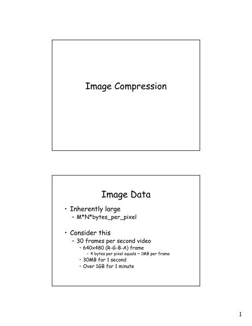
Image CompressionImage Data• Inherently large– M*N*bytes_per_pixel• Consider this– 30 frames per second video• 640x480 (R-G-B-A) frame– 4 bytes per pixel equals ~ 1MB per frame• 30MB for 1 second• Over 1GB for 1 minute1

Image Compression• We need a way to “compress” imagedata• Conserve bandwidth– For backing store (disk drive, CD-ROM)– Network transmissionData Compression•Two categories– Information Preserving• Error free compression• Original data can be recovered completely– Lossy• Original data is approximated• Less than perfect• Generally allows much higher compression2

Basics• Data Compression– Process of reducing the amount of datarequired to represent a given quantity ofinformation• Data vs. Information– Data and Information are not the samethingBasics• Data vs. Information–Data• the means by which information is conveyed• various amounts of data can convey the sameinformation– Information• “A signal that contains no uncertainty”3

Example of data vs.informationDataset 1 Dataset 2NxN imagecircle(0,0,r)NxN*1byte(pixel data)24*1 byte(24 ascii charactersto store the above text)Redundancy• Redundancy– “data” that provides no relevant information– “data” that restates what is already known• For example– say N1 and N2 denote the number of “dataunits” in two sets that represent the sameinformation– Relative redundancy of the first set of data N1 is• R D= 1 - 1/C r– where C r is the “Compression Ratio”• C r= n1 / n24

Redundancy• Relative Redundancy of N1 to N2– R D = 1 - 1/C r• Compression Ratio– C r = n1 / n2• if (n2 = n1)– C r = 1 , R D = 0• Compression Ratio is 1, implying there is no redundancy• if (n2

Compression• Given a set of N data units• Try to remove redundant data that isnot needed to express the underlyinginformation• Hopefully your new set, N’– N’

Coding Redundancy• Recall the Histogram–p r (r k ) = n k /n k=0,1,2, . . , L-1• L is the number of gray levels• n k is the number of pixels with gray level “r k ”• n is the total number of pixels• p r (r k ) is the probability that r k will occur in this image• Let L(r k ) = the number of bits needed torepresent the gray level r kCoding Redundancy• Let L(r k ) = the number of bits needed torepresent the gray level r k• The average number of bits needed torepresented each pixel is– Lavg = Σ L(r k ) p r (r k )• Thus, the total number of bits needed to code animage– N*M*Lavg7

Coding Redundancy• Example– Consider an image with 8 gray levels–L1(r k ) is a natural binary coding set• m-bit counting sequence ie (2 m )• thus, to encode 8 distinct codes needs m = 3– Each pixel uses 3 bits• Lavg = 3bitsCoding Redundancy• However, consider using the codes in this table• Lavg = Sum l 2 (r k )p r (r k ) =2(0.19) + 2(0.25) + 2(0.21) + 3(0.16) + 4(0.08) +5(0.06) + 6(0.03) + 6(0.02)Lavg = 2.7 bits8

Coding Redundancy• L1avg = 3 bits• L2avg = 2.7 bits• Cr = L1avg/L2avg = 3/2.7 or 1.1• Rd = 1 - /1.11 = 0.099• Thus approximately 10 percent of the data in L1 isredundant“Variable Length Coding”• Assigning fewer bits to more probablesymbols achieves compression• This process is commonly referred to as“variable-length-coding”• What is the pitfall?– Equally probable symbols• Generally no gain . .• Then don’t encode. . .– Need to know how to choose the “symbol”9

Variable Length Coding andCompression• If gray-levels of an image are coded using moresymbols than absolutely necessary• It is said to contain coding redundancy• Variable length coding is very powerful and isfrequently applied– Not just for images– Characters strings too• Gzip, Zip, etc use a form of variable length codingInterpixel Redundancy• Think of an average binary image• The value of a pixel can be reasonablypredicted from its neighbors• Sometimes called– Spatial Redundancy– Geometric Redundancy– Interframe Redundancy– Well call it “interpixel” redundancy10

Interpixel Redundancy• In order to reduce redundancy in 2D pixelarrays• We can convert them into more efficient,“non-visual” format• Transforms of this type are called“mappings”– they are reversible if the original imageelements can be reconstructed from thetransformed data setsRun-length Encoding• Each scan line, y, of an binary image f(:,y)is encoded as a sequence of 0 and 1sf(0,y) f(1,y) f(2,y) . . . f(n-1, y)• An alternative– encode as a pair of sequences– (g1,r1) (g2,r2) . . (gi,ri) . . . (gn,rn)– where g1 encodes the gray-level (0 or 1)– and ri encodes the “run” length in pixels11

ExampleThresholdExample• The entire image in previous example– 1024x343 pixels (1 bit)– required only 12,166 runs• each run requires 11 bits to encode– N1 = 1024x343 (the binary image)– N2 = 12,166 * 11 (run length encoded image)• Cr = (1024)(343)/(12,166*11) = 2.63• Rd = 1 - 1/2.63 = 0.62– N1 (the binary image) is roughly 62% redundant12

Psychovisual Redundancy• “Brightness” as perceived by the eye is dependent on manythings• The fact is, the eye does not respond with equal sensitivityto all visual information• Some information has less relative importance than otherinformation• This information is said to be psychovisually redundant– It can be eliminated without significantly impairing visual“quality”Psychovisual Redundancy• Unlike Coding and Interpixel Redundancy– Psychovisual is associated with real orquantifiable visual information– It is possible only because the elimination ofthis data does not effect the visual process• But we lose quantifiable information– Thus, this type of reduction is called“quantification”• And it is lossy13

Lots of examples• Improved Gray-Scale Quantization(IGS)• Maps 8 bits to 4 bits•Adds some random noise topixels before quantization•This noise helps removesour sensitivity to edgescreated by quantizationOriginalStraightQuantizationIGSQuantizationLots of examples• Color Quantization is very common• MPEG and (digital video) DV Standards–Terms like– 4:2:2• For every 4 intensity pixels– only 2 color pixels are stored(in X and Y direction)– 4:1:1• For every 4 intensity pixels– only 1 color pixels are stored(in X and Y direction)14

Temporal Interlacing• TV signal is interlaced• 1 frame is composed of “2 fields”– one with odd scanlines– one with even scanlines• Frame rate is 29.9 per second (NTSC)24 per second (PAL)– But ~60 fields per second are displayed– Exploits temporal and spatial coherency– progressive scan• Full frameInterlacingOddEven(De-interlacing)15

Fidelity Criteria• Psychovisual data reduction results ina loss of quantitative visualinformation• Because information of interest maybe lost– a repeatable or reproducible means ofquantifying the nature and extent ofinformation loss is desirableFidelity Criteria• Two class of criteria are used– Objective fidelity criteria– Subjective fidelity criteria•Objective– loss can be expressed as a function of• the input image and• the resulting compressed (thendecompressed) image16

Objective Fidelity Criteria• Let f(x,y) be the input image• Let f’(x,y) be the “approximated” f(x,y)from compression/decompression• For any value of x and y, the error e(x,y)between f(x,y) and f’(x,y) is– e(x,y) = f’(x,y) - f(x,y)Objective Fidelity Criteria• The total error between the two imagese =∑M − 1x=0∑N −1y=0[ f '( x,y)− f ( x,y)]• The Root-Mean-Square Errorerms=1M 1 12[ [ '( , ) ( , )]] − N −f x y − f x y21 ∑ ∑MNx=0y=017

Objective Fidelity Criteria• Commonly used fidelity criteria is– mean-square signal-to-noise ratiodefined as:SNRM−1N−1∑∑x=0 y=0ms=M−1 N−1∑∑[f '( xx=0 y=0f '( x,y)2, y)− f ( x,y)]2signalnoise(Mean squared error)Subjective Fidelity Criteria• Human-based criteria• Usually side-by-side comparison18

Image Compression Modelsf(x,y)SourceencoderChannelencoderChannelChanneldecoderSourcedecoderf’(x,y)f(x,y)MapperQuantizerSymbolEncoderSymboldecoderInverseMapperf’(x,y)LossError-Free ImageCompression(Lossless Compression)19

Error-Free Compression• To reduce only coding redundancy• Most popular technique is– Huffman Encoding• This is a variable-length coding technique– Huffman encoding yields the smallest possiblenumber of code “symbols” per source symbol• Optimal for a fixed number of source symbols• subject that source symbols are coded one at a timeHuffman Encoding• Huffman encoding• Perform a series of source reductions– Ordering the probabilities of the symbolsoccurrence–combine the lowest probable symbols into asingle symbol that replaces them in the nextreduction– assigns codes based on these reduction• This is “variable-length” coding• So, we will have to build variable-length codes20

Huffman Encoding(Reduction)a2a6a1a4a3a5Original SourceSymbolProbability0.40.30.10.10.060.0412Source Reduction34Huffman Encoding(Reduction)a2a6a1a4a3a5Original SourceSymbolProbability 10.4 0.40.3 0.30.1 0.10.1 0.10.06 0.10.042Source Reduction3421

Huffman Encoding(Reduction)Symbola2a6a1a4a3a5Original SourceSource ReductionProbability 1 230.4 0.4 0.40.3 0.3 0.30.1 0.1 0.20.1 0.1 0.10.06 0.10.044Huffman Encoding(Reduction)a2a6a1a4a3a5Original SourceSymbolSource ReductionProbability 1 230.4 0.4 0.4 0.40.3 0.3 0.3 0.30.1 0.1 0.2 0.30.1 0.1 0.10.06 0.10.04422

Huffman Encoding(Reduction)a2a6a1a4a3a5Original SourceSymbolSource ReductionProbability 1 23 40.4 0.4 0.4 0.4 0.60.3 0.3 0.3 0.3 0.40.1 0.1 0.2 0.30.1 0.1 0.10.06 0.10.04Code assignmentOriginal SourceSource ReductionSymProbCode1234a20.40.40.40.40.60a60.30.30.30.30.41a10.10.10.20.3a40.10.10.1a30.060.1a50.0423

24Code assignment0.04a50.10.06a30.10.10.1a4010.30.20.10.1a110.4000.30.30.30.3a600.610.40.40.40.4a24321CodeProbSymSource ReductionOriginal SourceCode assignment0.04a50.10.06a30110.10.10.1a4010.30100.20.10.1a110.4000.3000.30.30.3a600.610.410.40.40.4a24321CodeProbSymSource ReductionOriginal Source

25Code assignment0.04a501010.10.06a30110.101000.10.1a4010.30100.20110.10.1a110.4000.3000.3000.30.3a600.610.410.410.40.4a24321CodeProbSymSource ReductionOriginal SourceCode assignment010110.04a501010.1010100.06a30110.101000.101000.1a4010.30100.20110.10110.1a110.4000.3000.3000.3000.3a600.610.410.410.410.4a24321CodeProbSymSource ReductionOriginal Source

Huffman Encoding• Uniquely Decodablea2Symbol Table0.41• consider010100111100a6a1a40.30.10.1000110100a3a1 a2 a2 a6a3a50.060.040101001011Huffman Encoding• Very powerful encoding scheme• Produces the optimal codes– Given an input symbol set– And its known distribution• Need to store symbol table along withcompressed data!26

Error Free InterpixelEncodingRun Length Encodingd1 d2 d3We call this a “run”d1,d2,d3,d4,d5,d6,d7, . . . .Distances alternate between white and black27

Run-length coding variations•Divide image into 2D regions•If all white, assign a “1”•If all black, assign a “00”•Otherwise, code the block using sometechnique (1D RLE, etc)Previous RowRACRelative address codingc’Current RowecLook at white to black transitionsIn current row, position “c” is the first transitionThis run is length “ec”Examine previous row at position “c”Find the first transition before “c”, c’this distance is “c’c”28

Previous RowRACRelative address codingc’Current Rowec•Encode the smallest distance, d = min( ec, c’c )•You’ll need to a flag to denote which distance is used (1, or 0)•Need to handle boundaries•The idea is to reduce the number of bits needed to store the “run”Predictive Encoding• Consider a gray-scale image• Try to predict what a pixel’s value isgoing to be• Only encode the difference betweenthe predicted value and the real value29

Predictive Encodingf(x,y)+ ∑−e(x,y)CompressedImagePredictorNearest integerf’(x,y)e(x,y) = f(x,y) – f’(x,y)Predictive DecodingCompressedImagee(x,y)+ ∑−f(x,y)Predictorf’(x,y)30

Predictor• Various local, global, and adaptivemethods can be used• Most common is a linear combinationof “m” previous pixelsf'(m⎡x,y)= round ⎢∑αif⎣ i=1⎤( x − i,y)⎥⎦fixed weightsPredictorDifferential Coding• If previous pixel is used we call this“differential coding”•m=1 and α=1IEncode the differenceCan reduce “symbol” set sizeHelps variable length codingx31

ExampleOriginalf(x,y)e(x,y)Differential CodingInterpixel Coding Encoding• Interpixel coding– Is usually followed by variable-lengthcodingRLEorPredictiveHuffmanSource Encoder32

Image Compression Modelsf(x,y)SourceencoderChannelencoderChannelChanneldecoderSourcedecoderf’(x,y)f(x,y)MapperQuantizerSymbolEncoderSymboldecoderInverseMapperf’(x,y)LossImage Compression Schemes• Error Free Compression (often called “lossless” compression)• Data can be recovered completely• Some applications require this type of image compression– Medical imagery– Digital “Preservation”– Digital archives of black and white documents• However, most compression schemes allow for loss in orderto achieve high compression rates33

Next Lecture• Lossy Compression–Quantization– Transform-based compression• With Quantization•JPEG standard34