reciprocity and emc measurements - IEEE Electromagnetic ...

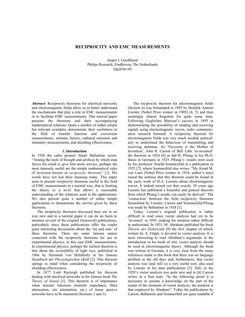
2you bear in mind that in their days the system of unitswas not the same as our current system.Ballantine, whose name lives on in the StuartBallantine Medal [9], published a most importantapplication of the field reciprocity theorem [10],referring to important work carried out by Raymond M.Wilmotte [11] of the National Physics Laboratory in theU.K. (Section 5). As we will show below, thisapplication leads to a hybrid reciprocity theorem that isof importance when considering antenna factors,radiated emission and immunity measurements, shieldingeffectiveness and uncertainties in EMC measurements(Section 6). Here the meaning of ‘hybrid’ is that,mathematically, the theorem is expressed in terms ofvoltage and current, on the one hand, and in electric andmagnetic field components, on the other hand.More recent literature on these reciprocity theoremscan be found in [12−15], for example, where dueattention is given to the mathematics. A contemporaryderivation of the hybrid reciprocity theorem used in thispaper can be found in [16], for example. The materialpresented here was published earlier in Dutch, in aseries of short articles in the journal of the DutchEMC/ESD Society [17].2. Kirchhoff networksThis section considers quasi-stationary linear passiveelectrical networks that do not contain devices thatmake use of the properties of magnetized ferrites, suchas circulators. If electric and magnetic fields play a role,their action is contained in lumped elements and/ornetwork parameters that describe field coupling such asthe mutual inductance. In other words, we considernetworks that obey the two Kirchhoff laws, so that inthe remainder of this paper we will refer to thesenetworks as Kirchhoff networks. The reciprocitytheorem discussed here interrelates two states of oneand the same Kirchhoff network, where the states aredetermined by the terminations of that network.U gI 1I 1AAZ 1 Z 2Z 3Z 1 Z 2Z 3Fig.1 Network to illustrate the reciprocity theorem.(a) e.m.f. U g at A and current measurement at B, (b)e.m.f. U g at B and current measurement at A.Lord Rayleigh, who formulated his reciprocity theoremrather generally in terms of forces and motions, presentsvarious applications [3] and writes:“A further example may be taken from electricity.Let there be two circuits of insulated wire A and Band in their neighborhood any combination of wirecircuits or solid conductors in communication withBBI 2I 2U g(a)(b)condensers. A periodic electromotive force in thecircuit A will give rise to the same current in B aswould be excited in A if the electromotive forceoperated in B”.This formulation hardly differs from that used todaywhen introducing this reciprocity theorem, normallyreferring to the two circuits shown in Fig.1:‘If an e.m.f. U g at the location A in a Kirchhoffnetwork causes a current I a 2 to flow at point B in thatnetwork then a current I b 1 = I a 2 will flow in point Aafter placing the e.m.f. U g at the location B in thatnetwork.’The superscripts a and b refer to the two states depictedin Figs. 1a and 1b. In more extended networks morethan one e.m.f. may be present that also contribute tothe current in the considered point. The theorem,however, only applies to that part of the current that iscaused by the considered e.m.f.. It is very easy to verifythat I b 1 = I a 2 by calculating both currents. It then followsthatZ3UagbI (1)2== I1Z Z + Z Z + Z Z12The given formulation of the reciprocity theorem is trueenough but it is not very suited for use in furtherconsiderations. The step is therefore made to the generalexpression that describes the reciprocity of an N-portKirchhoff network. As proven in [6, 18]NNa b∑UkIk= ∑k=1k=1where, again, the superscripts a and b correspond to twostates that are determined by the terminations of thenetwork and can be chosen arbitrarily within theconditions that apply. Equation (2) contains combinationsof the voltages in one state (a or b) and thecurrents in the other state (b or a). As such, Eq.(2) haslittle to say. It only comes alive when N and the states aand b have been chosen. Before doing so, Eq.(2) ischecked (not proven), in particular because the ‘recipe’used shows great similarities with the one used in thederivation of the expression describing the reciprocitytheorem for electromagnetic fields (see also Eq.(24)).The most simple network is a one-port (N= 1)formed by an impedance Z. In such a case Eq.(2)reduces to U a 1 I b 1 = U b 1 I a1 and the correctness of thisequation can be verified in a rather trivial way. Assumein the a-state the voltage across Z is given by U a 1 = ZI a 1 ,and in the b-state by U b 1 = ZI b 1 . The left and right handbmember of the first equation are now multiplied by I 1so that U a 1 I b 1 = ZI a 1 I b a1 and, equally, the second one by I 1so that U b 1 I a 1 = ZI b 1 I a 1 . Subtracting the second equationfrom the first one yields the relation beingdemonstrated: U a 1 I b 1 = U b 1 I a 1 .To check the general expression, Eq.(2) is firstwritten in vector/matrix formb T a[ I ] [ U ] = [ Ia(2)(3)where the subscript T denotes the transposed matrix. Inthis notation, Ohm’s law leads to [U a ]= [Z][I a ] in the a-state and to [U b ]= [Z][I b ] in the b-state. In a similar way23T] [ UUb]3bkI1ak

3as with the one-port, the first equation is multiplied by[I b ] T and the second one by [I a ] T . The result of thesemultiplications is (note that the order of the terms isnow always of importance)b T a b T a[ I ] [ U ] = [ I ] [ Z][I ]anda T b a T b b T T a[ I ] [ U ] = [ I ] [ Z ][ I ] = {[ I ] [ Z][ I ]}(4a)(4b)where in Eq.(4b) we have made use of the matrixproperty [X] T [Y] T [Z] T = {[Z][Y][X]} T . If [Z]= [Z] T , as isthe case in an N-port Kirchhoff network, Eq.(3) andhence Eq.(2) directly follow after subtracting Eq.(4b)from Eq.(4a).3. Applications (1)This section presents four examples that connect thereciprocity theorem for Kirchhoff networks to EMCmeasurements.The examples pay particular attention tothe transfer impedance, filter attenuation, the conversionof a differential-mode (DM) voltage into a commonmode(CM) current and to site attenuation. In allexamples Fig.2 applies and N= 2, but the applicationsare not limited to N= 2. For example, if cross-talkbetween parallel lines is considered, N= 3 or evenhigher may give useful information.port 1termination+ Kirchhoff +U 1 U 2−Network−Fig.2 A two-port Kirchhoff network with a terminationat each port that depends on the chosenapplication.If N= 2, Eq.(2) reduces toI 1 I 2Tport 2terminationWhen applying Eq.(5), the termination at port 1 (seeFig.3) in the a-state is a current source of strength I 1aand port 2 is open circuited, i.e. I 2 a = 0. In the b-state, acurrent source I 2 b terminates port 2 while port 1 is opencircuited, i.e. I 1 b = 0. Hence, Eq.(5) reduces to U 2 a I 2 b =U 1 b I 1 a or, expressed in the transfer impedances Z 12 andZ 21Z21U=Ia2a1aI2= 0U=Ib1b2 bI1= 0= Z(6)So the cable transfer impedance is reciprocal if the cablebehaves as a Kirchhoff network. The cable is alwayspassive and is always linear at most practical signallevels, as long there is no magnetic material in the cableconstruction. If magnetic material is used, the current(e.g. the CM current on the cable) must be verified tomake sure that it is so low that no saturation of themagnetic material results. When measuring the transferimpedance it is often very difficult, if not impossible, tosufficiently satisfy the condition I 1 b = 0 or I 2 a = 0 at highfrequencies, so that the measurement result has to becorrected for this non-zero current effect. Section 6.7 oninterference prediction demonstrates another applicationof the transfer impedance concept.3.2. Filter attenuationIn the case of filter attenuation measurements, a source(e.m.f. U g , internal impedance Z g ) is connected via afilter to the load impedance Z L . A well known questionrelated to filter attenuation is: ‘Does it matter which ofthe filter ports is connected to the source and whichport is connected to the load of that source?’ If the filteritself is not purely symmetrical, the EMC engineer willanswer that question with ‘Yes’, although he or she willnot be able to demonstrate this using a 50Ω measuringsystem (generator and voltmeter having equalimpedances, e.g. Z g = Z L = 50Ω). The latter can beverified as detailed below.12U +a b a b b a b a1I1+ U2I2= U1I1U2I2(5)Z gU 2 aU 1bZ gIn fact in Fig.1 N= 2 also applies. There U 1 b = U 2 a = 0and U 1 a = U 2 b = U g and substitution into Eq.(5) showsagain that I 1 b = I 2 a .3.1 Transfer impedanceThe transfer impedance is the ratio of the voltage(e.m.f.) induced in a current loop by the current inanother current loop. A typical example is the cabletransfer impedance that characterizes the EMC behaviourof a cable (the cable ‘leakage’).I 1aU 2aU 1ba-state b-stateFig.3 The two states when discussing the transferimpedanceI 2bU ga-stateb-stateFig.4 The two states when discussing the filterattenuationAssume that in the a-state port 1 is terminated by thesource and port 2 by the load, and the reversetermination holds in state b (see Fig.4). If U 0 is thevoltage across Z L in the absence of the filter, the filterattenuation A a = U a 2 /U 0 in the a-state and A b = U b 1 /U 0 inthe b-state. So here it is relevant to consider the ratioA a /A b = U a 2 /U b 1 . At the terminations the followingrelations are validaaU = U − I ZUUU1b2b1a2Z L= Uggb= −I1Z= −IZa2Z LLL1− Ib2ZggU g(7a−7d)

4From Eqs.(7c) and (7d) it follows that U 2 a /U 1 b = I 2 a /I 1band Eqs.(5) and (7) yieldAAabI=Ia2b1I=Ia1b2( Z( ZThe attenuation will be independent of the choice ofsource port and load port if A a /A b = 1. In all other casesA a /A b ≠ 1 and relative impedance values will determinethe choice of the source and load port of the filter [19].The condition A a /A b = U a 2 /U b 1 = I a 2 /I b 1 = 1 is met ifI b 2 =I a 1 and/or Z g = Z L . It is well known that the conditionI b 2 = I a 1 , that simultaneously makes I a 2 = I b 1 , is met in thecase of a purely symmetrical filter; the reciprocitytheorem was not needed to demonstrate this. However,the condition Z g = Z L resulting in A a /A b = 1 is sometimesoverlooked as noted in Section 6.3. Moreover, it is thiscondition that explains why the engineer will measureno difference in the attenuation if source and load portare interchanged when using a 50Ω measuring system.Of course, another path could also have beenfollowed to arrive at the two conditions representingA a = A b . The Kirchhoff network can be characterized bya T-network and U a b2 /U 1 can be expressed in thenetwork impedances Z 1 , Z 2 and Z 3 (see Fig.1). Afterstraight forward calculations it then follows thatUUa2b1Z2Z=Z Z1LL(8)(9)where Z 2 = Z 1 Z 2 +Z 2 Z 3 +Z 3 Z 1 +Z 3 Z g +Z g Z L +Z 3 Z L . The conditionZ 1 = Z 2 then represents the purely symmetricalfilter and, again, the condition Z g = Z L represents the50Ω measuring system.3.3. DM/CM conversionThe application of a reciprocity theorem may change anunsuccessful measurement into a successful one. Anexample is the measurement of the conversion of adifferential-mode (DM) voltage into a common-mode(CM) current to characterize the emission properties ofa telephone subscriber line or a power line to which adigital-signal is applied. The DM voltage U DM issupplied by the digital signal, and the resulting CMcurrent I CM is a direct measure of the radiated emissioncapability of such a line. This measure can be expressedin a conversion admittance Y CM = I CM /U DM .To measure this conversion over a certain frequencyrange, e.g. 0.1 MHz − 30 MHz, it seems rather obviousto apply a DM voltage to the line and to measure theresulting CM current. However, the line is also arelatively efficient receiving antenna and ambient fieldswill induce CM currents that may be of the same orderof magnitude as the CM currents being measured, orpossibly even larger. Another problem might be thecorrect measurement of a DM voltage at the higher endof the frequency range. Both problems can becircumvented by applying a CM voltage U CM to the lineand measuring the resulting DM current I DM , i.e. bydetermining the conversion admittance Y DM = I DM /U CM .The reciprocity theorem can now be used to find thecondition leading to Y CM = Y DM .gg+ Z Z+ Z12− Z− ZZggLL+ Z+ Z) −U) −U22ggZ gU gCM-portU CMDM-portI DMa-stateb-stateFig.5 The two states when discussing the DM/CMconversionThe line being characterized can be considered as a twoportnetwork where port 1 is the CM port and port 2 theDM port, see Fig.5. The following choice ofterminations in the a- and b-state is now possible. Instate a, representing the determination of Y DM , port 1 isterminated by the voltage generator and a highimpedance FET probe measures U a 1 = U CM . Port 2 isshort-circuited (U a 2 = U DM = 0) and a current probearound the short circuit measures I a 2 = I DM . In state b,representing the determination of Y CM , port 2 isterminated by the generator and port 1 by the shortcircuit. In this case Eq.(5) reduces to U a 1 I b 1 = U b 2 I a 2 , sothatICMIDMY(10)CM= = = YDMU UDM UCM= 0CM-portI CMCM U DM = 0DM-portU DMA practical way of measuring Y DM is to use Macfarlane’sprobe [20]. As described in [21], the CMvoltage is applied to the CM input of the probe. Thevoltage is measured via a high impedance FET probe atthis input and the current is measured in the short circuitbetween the probe’s two DM terminals. Reference [21]also gives measured Y DM data.3.4. Site attenuationAlthough only voltages and currents have beenconsidered above, it does not mean that the reciprocitytheorem does not apply if electric and magnetic fieldsplay a role in the signal transfer. This should already beclear from the given examples, as field couplings playan important role in each of these examples.Another example is the determination of the siteattenuation in which the signal transfer between twoantennas above a reflecting plane is considered.Fortunately, the signal transfer can be modelled into apassive two-port network [22] containing linearimpedances as already described by Brown and King in1934 [23]. Using a 50Ω measuring system, we canconclude from the discussion in Section 3.2 that it is notimportant which port is connected to the generator andwhich one to the receiver as long as the antennas havefixed positions. However, as noted in Section 6.2, thisconclusion might not always be correct if the so-callednormalized site attenuation is considered4. Electromagnetic fieldsThis section considers the Lorentz reciprocity theoreminterrelating the electromagnetic fields in two states thatcan occur in one and the same domain in space. UsingCarson’s formulation [24] and today’s notation thereciprocity theorem for fields reads:Z gU g

5“If E a , H a are the field vectors due to a periodicdisturbance from a source A 1 located at O 1 and E b , H bare the corresponding field vectors due to adisturbance originating in A 2 from a source located atO 2 , then∫1+2( Ea× Hb) ⋅ds =1+2( E× H) ⋅ds(11)the surface integrals as indicated by the subscripts 1+2being taken over closed surfaces 1 and 2 surroundingthe sources A 1 and A 2 respectively.”Not directly given in [24] is the additional equality alsofollowing from the reciprocity considerations∫D( Ea⋅ Jb(12)where D is the volume containing the sources A 1 and A 2represented by the source vectors J a and J b , respectively.In Eq.(11) the surface of D is indicated by thesubscripts 1+2. Equation (12) will be used in thederivation of the hybrid reciprocity theorem in Section5. As will be noted below, Eqs.(11) and (12) areconnected to a special case of the general reciprocityrelation Eq.(19).So the theorem combines two field states (a and b),comparable to the discussed reciprocity theorem for anN-port Kirchhoff network. The derivation of Eqs. (11)and (12) starts from sets of two Maxwell’s equationsexpressed in the frequency domain for the states a andb:aacurlE= − jω µ Haa a(13a,b)curlH= + jωεE + JandbbcurlE= − jω µ Hbb b (14a,b)curlH= + jωεE + JNow the trick is to remember the existence of the vectorrelation div(X×Y)=Y⋅curlX−X⋅curlY and to writediv(div(EEab× H× Hba) = H) = H(15)(16)An expression for H b ⋅curlE a in Eq.(15) can be found bymultiplying the left and right hand members of Eq.(13a)by H b (be careful with the order of the variables)H(17)In a similar way, expressions can be found for the otherterms on the right hand side of Eqs.(15) and (16) bymultiplying Eqs.(13b), (14a) and (14b) by the propervectors. After substitution of all resulting expressions inEqs.(15) and (16) and subtracting the two finalequations, we find thatdiv(18)This equation, in which the ω-terms no longer appear, issometimes called the local form of the reciprocitytheorem. To find the general form, Eq.(18) has to be∫∫b a)dv = ( E ⋅ J ) dvbaD⋅curlE⋅curlEba⋅ curlE= − jω µabHb− E− Ebab⋅ Ha⋅curlH⋅curlHa b b a b a a b( E × H − E × H ) = E ⋅ J − E ⋅ Jabaintegrated over the volume D containing all sourcesrepresented by J a and J b , yieldinga b b a∫ div( E × H − E × H ) ⋅Da b b a∫ ( E × H − E × H ) ⋅dsSb a a b∫ ( E ⋅ J − E ⋅ J ) ⋅dvDd v =(19)We had to expect an integration as the Maxwell equationsconsider field derivatives whereas an expressionfor the fields is needed. The most left hand member ofEq.(19) has been converted from an integral over avolume D into an integral over the surface S of D byapplying Gauss’s theorem. This action also ‘removes’the div operation. Equation (19) is the general form ofthe Lorentz reciprocity theorem, a form that can even beextended [14], although this extension is not needed inthe context of this paper.A special case is the situation in which the relationbetween the E and the H vector of the field is fixed,such as in the far-field of an antenna. Then the outcomeof the integrals in Eq.(19) is equal to zero, a value givenby Lorentz as he considered the propagation propertiesof light. In the far-field, the field propagates as a planeor quasi-plane wave so that the E and the H vector ofthe field are perpendicular to each other and have aconstant ratio, η=√(µ/ε), the wave impedance (377 Ω inair). In vector notation the latter means that ν×E= ηH,where ν is the unit vector perpendicular to the planeformed by E and H. After application of this relation toE a ×H b and to E b ×H a and after application of the vectorrelation X×(Y×Z)= Y⋅(X⋅Z)−Z(X⋅Y) we find thata b b aE × H = E × H = η(E(20)a b b aso that E × H − E × H = 0 and, consequently,the integrals in Eq.(19) are equal to zero and Eqs.(11)and (12) given at the start of this section automaticallyfollow.5. The hybrid reciprocity theoremThe experimentalist can only humbly lift his hat at themathematical fireworks presented in Section 4 and thenpass to the order of the day. An application is what isneeded to catch his or her interest. As mentioned in theintroduction, a very useful application was alreadygiven in 1929 by Ballantine [10], referring to the workof Wilmotte [11].This application, resulting in thehybrid reciprocity theorem, can also be found in Section4.5 of a more recent textbook [16]. The theorem givesan expression for the voltage U i induced by an incidentfield E i in an antenna or structure acting as an antenna,e.g. an EUT (Equipment Under Test) and its connectedcables. Since the transmission and reception ofelectromagnetic waves is of interest in EMC fieldmeasurements, the two states a and b will now bedenoted by t (of transmission) and r (of reception).In the following, two wire antennas A 1 and A 2 areconsidered (see Fig.6). Each wire antenna consists ofb⋅ E=a)

6I 0U iFig.6 The states (a) transmission and (b) reception. Thedashed lines indicate parts that need notnecessarily be accessible.two wire elements, separated by a small gap of width w,that determines the distance between the two terminals(each connected to a wire element) of the antenna. Thewire antennas of total length L 1 and L 2 are assumed tobe electrically thin and perfectly conducting. The widthw

7e) Equation (23) can also be written astI ( l)iUi= ∫ E ⋅ d lIL10(25)so that I t (l)/I 0 can be considered to be the normalizedcurrent distribution in the transmitting state that weighsthe contributions of incident field in the receiving state.6. Applications (2)This section presents a number of simple applications ofEq.(23) or Eq.(25), dealing with the antenna factor,radiated immunity measurements and shielding.Interesting and rigorously treated applications ofEq.(24) can be found in [15, 25]. Only in simple casescan the integral in Eq.(23) or Eq.(25) be solvedanalytically; an example is given in Section 6.1.However, the other examples will show that quite usefulinformation is made available without solving theintegral.6.1. The λ/2-dipoleA very simple application of Eq.(25) follows if wecalculate the voltage induced in a λ/2-dipole in freespace. As can be found in all current text books onantennas and was verified experimentally by Wilmottein 1927 [26], the current distribution in the transmittingstate of this antenna is half a sine wave. If the incidentfield is a plane wave of strength E i with its polarizationparallel to the wire elements, the well known expressionfor the induced voltage follows from Eq.(25):UiE=Ii λ / 4∫I0 −λ/ 402πλ λsin( ( − l))dl= Eλ 4 π(26)If Z m is the effective load impedance and Z a the internalimpedance of the λ/2-dipole antenna, the voltage U mmeasured by the receiver is given byZmλ iU(27)m=Z + Z π Emand if E i = E c i is the field strength during calibration ofthis antenna, its antenna factor F A is given byFA(28)By stating ‘Z m is the effective load impedance of theantenna’ and not ‘Z m is the input impedance of thereceiver’, the properties of the antenna balun areassumed to be taken into account.Seibersdorf, for example, is a supplier of a set of 27λ/2-dipole antennas suitable for performing thevalidation of an antenna calibration test site as describedby CISPR/A [27]. For these antennas Z m = 100 Ω, andthe free space value of Z a = 73 Ω. Inserting these valuesin Eq.(28) results in F A values that differ less than 0.1dB from the theoretical values supplied by Seibersdorf(maybe, Seibersdorf also used Eq.(28)).aπ( Zm+ Z=λZma)i6.2. The antenna factor F AThis section should clarify which parameters play a rolein the determination of the antenna factor and what theconsequences are in radiated emission measurements,measurement uncertainty and normalized siteattenuation measurements.By definition, the measured field strength E m =F A U m , so the antenna factor can be written as(29)The antenna factor therefore depends on 3 variablesdetermined by the calibration set-up, in Eq.(29)indicated by the subscript c,1) The antenna impedance Z a,c ,2) The normalized current distribution I c t (l)/I 0 , and3) The outcome of the dot-product E c i ⋅dl along thewire elements.As a consequence, if in a radiated emission measurementone or more of these three variables differ fromthe values during calibration, the antenna factor isunknown. In discussions about the standardization ofradiated emission tests, the first variable (the antennaimpedance) has often been considered, but not the othertwo variables.The normalized current distribution depends on theinteraction of the antenna with its environment duringits actual use (calibration or radiated emission test). Ofcourse, the outcome of the integral depends on theincident-field distribution which, however, is notspecified in a radiated emission compliance test. Thewire elements of a receiving antenna automatically‘integrate’ over the field distribution whether themeasurement is carried out on an open area test site, orin a semi or a fully anechoic room. Consequently,antennas with different shapes will have differentinduced voltages, even if the incident field is a planewave.∆FA (dB)2,52,01,51,00,5Fig 7.FAZ=m+ ZZma,c∫Lti( I ( l) / I )E ⋅dlThe difference ∆F A = F A (ANSI/3m)−F A (Free-Space) between the antenna factors of a logbiconicalantenna derived from the twocalibration reportsThe combined effect of all three variables comes to thefore in the first example. Figure 7 shows the difference∆F A between the ANSI(3m) antenna factor and the free-c0,00 50 100 150 200 250 300Frequency (MHz)10c

8space antenna factor of one and the same log-biconicalantenna, as determined by a UKAS accredited company.We can also conclude from the above that thelinearized model used in documents on EMCmeasurement instrumentation uncertainties [28, 29]cannot be justified. Moreover, the uncertainty in theantenna factor during calibration has little in commonwith the uncertainty in the antenna factor during anactual radiated emission test. In the normalized siteattenuation measurement method the result of the siteattenuation measurement is normalized to the antennafactors, after which the result is compared to atheoretically predicted result. This method is formallyonly correct if it can be demonstrated that the antennafactors used are valid during the conditions of the siteattenuation measurement.As a second example, Fig.8 shows the differencedE max when in the CISPR/A radiated emission roundrobin test (RRT) the field-strength emitted by thebattery operated tightly specified EUT (a rod antennaabove a small ground plane) was firstly measured usinga biconical antenna and secondly by using a logbiconicalantenna [30]. When replacing the receivingantenna, care was taken that the remaining part of theset-up was not changed. Only the prescribedmeasurement distance was adjusted by moving thereceiving antenna. In this example, the effect ofintegrating over different parts of the incident fielddistribution comes to the fore very clear. This effect wasalso found in the statistical evaluation of the RRT fieldstrength measurement results using the tightly specifiedEUT [30].dEmax (dB)30−30 100 200 300Frequency (MHz)Fig.8 Measured field strength difference dE max (dB)after a biconical antenna has been replaced by alog-biconical antennaWhen using a log-biconical antenna, the effectivemeasurement distance changes with frequency, and ithas sometimes been suggested that is possible to correctfor this effect. From the theory above, it will be clearthat such a correction is only possible if the completeactual incident-field distribution is known andaccounted for in the correction factor.6.3. Probe calibration in a TEM cellField probes are often calibrated in a TEM-cell. However,the practical use of these probes is generallyoutside such a cell. So the current distribution in the t-state, and, consequently, the antenna factor, may bedifferent in cases where the probe is not as close to themetal plates as it is inside the TEM-cell. It seems thatthis aspect was overlooked in [31]. It might therefore beone of the reasons for the limited agreement betweenmeasurement results obtained in the TEM cell and thoseobtained outside that cell. In addition, the authors in[31] claim that the reciprocity of the TEM cell wasverified experimentally. In that experiment, a firsttransfer function was measured after connecting thesignal generator to the probe acting as transmittingantenna inside the cell and the measuring receiver toone of the cell terminals. A second transfer function wasmeasured after reversing the connections, i.e. afterconnecting the generator to the cell terminal and themeasuring receiver to the probe. They then concludethat reciprocity has been demonstrated as the twotransfer functions differed by less than 1 dB. However,for trivial reasons the TEM cell was a linear passivedevice and, hence, was reciprocal. The discussions inSection 3.2 then indicate that the experiment onlydemonstrated that the ratio of the output impedance ofthe generator and the input impedance of the measuringreceiver was smaller than 1 dB. If a 50Ω generator and a75Ω measuring receiver would have been used, for example,that ratio would most likely have been differentand the authors would have discovered that their methodneeded an additional consideration.Another application of the reciprocity theorem involvinga TEM cell is given in [32].6.4. Radiated immunity, E iIn a radiated immunity test, it is the induced voltage thatmay cause malfunctioning of the EUT. Equation (25)clearly indicates that this voltage is determined by theincident field and by the normalized currentdistribution. In this section, aspects of the incident fieldare considered and in Section 6.5 aspects of the currentdistribution are considered.The incident field is the field that would be presentin absence of the EUT plus its attached cables acting asan antenna. Consequently, the specified field strength ina radiated immunity test is normally measured andadjusted before the placement of the EUT using a smallprobe (negligible interaction with the field source). It isnot correct to measure the specified field strength usinga small probe near the EUT, because that probemeasures the field incident to the probe. The latter fieldmay significantly differ from the incident fieldexperienced by the EUT, as it is the combination of thewanted field and the field reflected from the EUT. Thefield incident to the probe might even be almost zero ifthe desired test field and the reflected field are in antiphase.After placement of the EUT we need to verify thatthe incident field as such has not changed as a result of apossible strong interaction between the EUT and thesource of the field. Such an effect may be observed bycomparing the forward power measured via adirectional coupler, in the connection between thegenerator and antenna emitting the test field during thepreviously mentioned field adjustment, with the powermeasured after the placement of the EUT. If the forwardpower has changed, the desired incident field haschanged. A first correction is to adjust the generatoroutput to a level that results in the original forwardpower. However, from the hybrid theorem it followsthat this adjustment does not need to be 100% correct,

9as the field distribution during the field adjustment andthat after placement of the EUT need not be the same.6.5. Radiated immunity, I t (l)/I 0Equation (25) also indicates that the normalized currentdistribution in the t-state is of importance. Since thatdistribution is the weighting function of the voltagecontributions induced by the incident field, resonancesin that distribution may be noticed in the disturbancesignal induced in the cable attached to an EUT. Anexample is given in Fig.9, where the maximum (max),average (avg) and the minimum (min) value of themeasured induced CM-current are plotted as a functionof the frequency of the homogeneous incident field witha strength of 1 V/m. Eight EUTs taken from a class ofelectrically small EUTs were tested [21].CM-current dB(µA)806040maxavgmin200 50 100 150 200Frequency (MHz)Fig.9 The induced common-mode current measuredclose to an electrically small EUT in the cableattached to that EUT, when illuminated by a fieldof 1 V/m (8 EUTs)Although the average value is about 55 dBµA (a valueclose to the rule of thumb for these EUTs: 1 mA perV/m), the curve labelled ‘min’ indicates that resonancesmay cause a minimum in the induced current, so that theconsidered EUT is hardly tested for immunity aroundthe resonance frequencies. In other words, a uniformand constant incident field does not guarantee that theEUT is tested with a constant actual disturbance signal(here represented by the CM current). In addition, weshould expect the resonance frequencies to shift whenthe layout of the cables is changed. If it had beenpossible to let the EUT act as a transmitter, theresonances would also have been found, comparable tothe resonances of a rod antenna.In the case of an interference complaint in which aproduct is insufficiently immune to EM fields, it is notalways possible to solve the problem at the locationwhere the product is used. The disturbance fieldstrength at that location is measured and the product istaken to the test lab to carry out a radiated immunity testwith that field strength. However, if the CM currentdistribution on the cables attached to that product differssignificantly in the test situation from that at thecomplaint location, the test might not cover the actualcomplaint. So it is advisable to measure not only thefield strength at the complaint location, but also the CMcurrent on the attached cables (close to the product) andto verify whether these currents are (more or less) thesame in the test house.6.6. ShieldingThis section addresses the frequently asked question ‘Ifa shield attenuates the field emanating from circuitsinside that shield by an amount of X dB, are thesecircuits then also shielded by an amount of X dB forfields generated outside that shield?’ We can illustratethe reasoning behind the answer by the following rathersimple configuration, that allows the use of simpleanalytical relations. Rigorous approaches based on theLorentz theorem can be found in [25, 33]. In Section 6.7the results are also used in an example of interferenceprediction.RD aLoop antenna+Screenrλ/2-antennaFig.10 Schematic drawing for use in the application ofthe reciprocity theoremsA tuned λ/2 dipole is located at a distance r in the farfieldof a small loop antenna, as shown in Fig.10. Bothantennas are located in free space so that antennacoupling and reflections do not play a role. A signalsource {U g , R g } can be connected to the loop antenna,and a voltmeter (input impedance R v = R g ) can beconnected to the λ/2 dipole (internal impedance Z a ), andvice versa. The area of the loop antenna A= πD a 2 /4 andthe internal impedance of that antenna is Z l . Theorientation of both antennas is such that an optimalsignal transfer results.If the source is connected to the loop antenna andthe voltmeter to the λ/2 dipole, the voltmeter readingU v1 in the absence of the screen will be given byUv1=π(2λ RgZ0k AUg⋅R + Z ) 4π r(R + Z)ga(30)where λR g /{π(R g +Z a )}is the voltmeter reading in thecase of an incident field given by the second part of theright hand member of Eq.(30), (also see Eq. (27)). Inthat part, AU g /(R g +Z l ) is the magnetic dipole moment ofthe loop antenna, Z 0 the far-field wave impedance andk= 2π/λ. Next, a spherical screen of radius R,D a /2

10Eq.(30), although the magnetic dipole moment is now afactor S H smaller.The next step is to connect the generator to the λ/2dipole and the voltmeter to the loop antenna. In theabsence of the screen U v3 is measured and in thepresence of that screen U v4 is measured. The voltage U v3is given byUv3µ0ωARg2Ug= ⋅( Rg+ Z)4πr(Rg+ Za)(31)where R g /(R g +Z l ) gives the voltage division of thevoltage µ 0 ωAH induced by the incident H-field. Thatfield is given by the second part of the right handmember of Eq.(31), and is easily understood whenremembering that in the far-field the E-field of a centerfed tuned λ/2 dipole is given by E= 60I/r= 2Z 0 /(4πr) sothat H= 2I/(4πr) and where I is the current entering theantenna.Using the relations Z 0 = √(µ 0 /ε 0 ) and f⋅λ = c =1/√(µ 0 ε 0 ) we can easily verify that U v1 = U v3 . This is nota surprising result, since the equivalent networkbetween the ports of the two antennas is a Kirchhoffnetwork, which means that the associated reciprocitytheorem directly gives the answer U v1 = U v3 (see Eq.(8))using Z g = Z L = R g . However, because the screen is alsolinear and passive, the same theorem shows that U v2 =U v4 , and a simple calculation like the one above todemonstrate this result is not possible. The laststatement is particularly true because the dipole fieldarrives as a plane wave at the screen, while the screen isin the near-field region of the loop antenna. Aknowledgeable in the theory may be able to show thatthe Helmholtz theorem about the reversibility of lightrays [2] is applicable in the described situation.In this example the actual shielding effectivenessis determined by that of the screen in the near-field ofthe loop antenna. This effectiveness is generally muchlower, e.g. 40 dB, than that for a plane wave generatedoutside the screen. The example stresses the fact that theshielding effectiveness is not entirely a property of theshield. It is a property of the shield plus the antennas orantenna structures playing a role in the disturbancesignal transfer.In conclusion, the reciprocity theorems give conditionsunder which the shielding effectiveness isreciprocal, and the results are certainly applicable in thecase of in-band interference. In the case of out-of-banddisturbances acting on non-linear devices such astransistors, the theorems are not formally applicable.However, it is still possible to follow the given path toestimate the magnitude of the induced signals and toconsider the consequences of those signals afterwards[33].6.7. Interference predictionThe results obtained in Section 6.6 can be applied tointerference prediction. As an example, the followingapplication considers the unwanted signal induced by adistant broadcasting transmitter in the antenna ofMagnetic Resonance Imaging (MRI) equipment used inhospitals.In the early days of the use of MRI equipment,hospitals did not like to have large Faraday cagesaround the equipment. As broadcasting transmitterscould emit strong fields at the in-band frequencies of theMRI equipment, the following question arose ‘Is itpossible to carry out field strength measurements at thelocation where the MRI equipment is planned to be usedbefore the placement of that equipment and to predictthe level of the disturbance signal induced in the MRIantenna?’ The answer was ‘Yes, and with a reasonabledegree of confidence’. The following three steps had tobe followed to find the answer. Figure 10 is againapplicable: the MRI antenna is the loop antenna and theλ/2 dipole is the antenna of the broadcasting transmitter,(normally a λ/4 antenna above the earth acting as aground plane). Simple mathematical relations illustratethe estimate of the maximum voltage U i,max that could beinduced in the loop antenna.Step 1: Connect a signal source {U g , R g } to the MRIantenna located at its normal-use position inside theMRI equipment, so that all interactions are properlytaken into account. Set the frequency of this source tothat of the (strong) broadcasting field to be expected inthe hospital. Measure at a distance r 1 in the far-field ofthe MRI equipment the field pattern E 1 (φ), 0°≤φ≤360°,emitted by the MRI antenna and measure the current I 0tflowing into the loop antenna. This is a measurementthat can be carried out on the manufacturers premises!Step 2: Determine the maximum E max of E 1 (φ) andassume that the MRI equipment emits this field in thedirection of the λ/2 dipole at a distance r from theequipment (worst case). This field is proportional to I 0 t ,so E max = α max I 0 t and the incident field for the λ/2 dipoleE t = (αr 1 I 0 t )/r. Application of the hybrid reciprocitytheorem then gives the voltage induced in the λ/2dipole: U i , λ/2 = (α max λr 1 I 0 t )/(πr), (see Eq.(26)). Consequently,the transfer impedance Z tr between the loopantenna and the λ/2 dipole is given byZαmax 1tr=λ rπ r(32)and in the given situation Z tr is reciprocal.Step 3: During operation of the broadcastingtransmitter, the input current to its antenna is I 0 r and thatcurrent can be determined from the field strength E rmeasured at the location where the MRI equipment is tobe installed, by using the well known relation E r =60I 0 r /r. Using Eq.(32), the estimate of the maximumvoltage U i,max induced by the broadcasting transmitter inthe loop antenna is given byUi,max= ZIrtr 0αmaxλr1= E60π(33)By comparing this voltage with the level allowed tooperate the MRI equipment sufficiently free ofinterference, a decision can be made about whether ornot a Faraday cage is needed and, if it is, how muchattenuation that cage should present.r

11SummaryIn this paper we have discussed the reciprocity theoreminterrelating two states of one and the same Kirchhoffnetwork (linear passive network) as determined by theterminations of that network. We have givenapplications improving the understanding of transferimpedance, filter and site attenuation measurements. Inaddition, we have used the theorem to facilitate a DMvoltage to CM current conversion measurement.We discussed the reciprocity theorem interrelatingthe electromagnetic fields in two states that can occur inone and the same domain in space, and from thistheorem we derived the hybrid reciprocity theorem. Thelatter theorem was applied to a tuned λ/2 dipole, to themeasurement of antenna factors, to probe calibration ina TEM cell and the uncertainties associated with thesemeasurements. We also used the hybrid reciprocitytheorem to discuss aspects of radiated immunitymeasurements.Finally, we used the reciprocity the reciprocitytheorems in a discussion about the reciprocity of theshielding effectiveness and in a simple method toestimate the interference potential of a field (at in-bandfrequencies) incident on an antenna.AcknowledgementsThe author wishes to acknowledge the valuable andinteresting discussions with Dr. Stef Worm of PhilipsEMC Competence Centre in Eindhoven. He also wishesto thank the library staff at Philips Research in Eindhoven.The presence of all historical publications in thelibrary’s collection made his nostalgic journey a pleasant‘one-stop’ event.References[1] S. Ballantine, “The Lorentz Reciprocity Theoremfor Electric Waves”, Proc. IRE, vol.16, pp 513−518, 1928.[2] H. von Helmholtz, Handbuch der PhysiologischenOptik (1866); Verlag von Leopold Voss, Hamburg/Leipzig,3e Auflage, pp 200−203, 1909.[3] J.W. Strutt, Baron Rayleigh, The theory of sound,vol. 1, pp. 150−157, 1877; reprinted by Mac-Millan, London, 1926.[4] H.A. Lorentz, “Het theorema van Poynting over deenergie van het electromagnetisch veld en een paaralgemene stellingen over de voortplanting van hetlicht”, Verslagen Kon. Akademie van Wetenschappen,Band 4, p.176, Amsterdam, 1896.[5] H.A. Lorentz, “The theorem of Poynting concerningthe energy in the electromagnetic field andtwo general propositions concerning thepropagation of light”, Collected papers, Nijhoff,Den Haag, vol. III, p 1, 1936.[6] J.R. Carson, “A generalization of the reciprocaltheorem”, Bell Syst. Techn. Jrnl., vol. 3, pp 393−399, July 1924.[7] A. Sommerfeld, “Das Reziprozitäts-Theorem derdrahtlosen Telegraphie”, Zeitschrift für Hochfrequenztechnik,Band 26, Heft 4, pp 93−98, 1925.[8] M. Abraham, Theorie der Elektrizität, TeubnerVerlag, Berlin, 1921.[9] The Stuart Ballantine Medal, to be awarded inrecognition of outstanding achievement in thefields of Communication and Reconnassancewhich employ electromagnetic radiation, TheFranklin Institute, Philadelphia, U.S.A.[10] S. Ballantine, “Reciprocity in electromagnetic,mechanical, acoustical, and interconnectedsystems”, Proc. IRE, vol. 17, pp 929-951, June1929.[11] R.M. Wilmotte, “The nature of the field in theneighbourhood of an antenna”, Journ. IEE, vol. 66,pp. 961−967, 1928.[12] C.T. Tai, “Complementary Reciprocity Theoremsfor Two-Port Networks and Transmission Lines”,IEEE Trans. on Education, vol. 37, no.1, pp42−45, 1992.[13] C.T. Tai, “Complementary Reciprocity Theoremsin Electromagnetic Theory”, IEEE Trans. onAntennas and Propagation, vol.40, no.6, pp675−681, 1992.[14] A.T. de Hoop, Handbook of radiation andscattering of waves, Academic Press Ltd., London,1995.[15] D. Quak, “Electromagnetic Susceptibility Analysisof Open-Wire Systems”, Proc. IEEE Intern. Symp.on EMC, Atlanta, pp 423−428, August 1995.[16] K.F. Sander and G.A.L. Reed, Transmission andpropagation of electromagnetic waves, CambridgeUniversity Press, Cambridge, 1986.[17] J.J. Goedbloed, “Reciprociteit en EMC-metingen”,EMC/ESD Praktijk, 1) pp.5−7, Sept. 2001, 2) pp5−7, Okt. 2001, 3) Elektronica, EMC/ESD Praktijk,pp. 5−7, Nov. 2001, “Over het afschermen vanvelden (4)”, Elektronica, EMC/ESD Praktijk, pp.44−45, Mei 2002.[18] B.D.H. Tellegen, “A general network theorem,with applications”, Philips Research Reports, 7,pp259−269, 1952.[19] J.J. Goedbloed, Electromagnetic Compatibility,Kluwer Technische Boeken, Deventer, 1997 (originallypublished by Prentice Hall, 1992).[20] I.P. Macfarlane, “A Probe for the Measurement ofElectrical Unbalance of Networks and Devices”,IEEE Trans. on EMC, vol. 41, pp. 3−14, Feb.1999.[21] J.J. Goedbloed, “Aspects of EMC at the equipmentlevel”, Proc. Intern. Symp. on EMC, Zurich, Suppl.pp 23−38, 1997 and IEEE Intern. EMC Symposium,Austin, U.S.A., 1997.[22] A. Sugiura, “Formulation of Normalized SiteAttenuation in Terms of Antenna Impedances”,Trans. IEEE on EMC, vol. 32, pp. 257−263, Nov.1990.[23] G.H. Brown and R. King, “High frequency modelsin Antenna investigations”, Proc. IEE, vol. 22, pp.457−480, April 1934.[24] J.R. Carson, “Reciprocal theorems in radio communication”,Proc.IRE, vol.17, pp 952-956, June1929.[25] D. Quak and A.T. de Hoop, “Shielding of WireSegments and Loops in Electric Circuits by

12Spherical Shells”, Trans. IEEE on EMC, vol. 31,pp 230− 237, August 1989.[26] R.M. Wilmotte, “The distribution of current in atransmitting antenna”, Jour. I.E.E., vol. 66, pp617− 627, 1928.[27] Specification for radio disturbance and immunitymeasuring apparatus, CISPR Publ. 16-1, 2 nd Ed.,pp 107-133, 1999.[28] Accounting for the measurement uncertainty whendetermining compliance with a limit, CISPR Publ.16-4, 2002.[29] The treatment of uncertainty in EMC measurements,NAMAS Publication NIS81, May 1994[30] J.J. Goedbloed, “Analysis of the results of theCISPR/A radiated emission round robin test”, Nat.Lab. Unclassified Report 2002/811, May 2002,Philips Research, Eindhoven, The Netherlands.[31] D.J. Groot Boerle, F.B.J. Leferink and T.D. Leistikow,“Obtaining the antenna factor of an opticallydriven antenna using the reciprocity of a TEMcell”, IEEE EMC Symposium, pp 900−905, 1998.[32] S.B. Worm, Comparison of workbench methodsfor testing RF emission properties of integratedcircuits, Proc. Intern. Symp. on EMC, Zurich, pp673−678, Febr. 2001.[33] B.L. Michielsen, “A new approach to electromagneticshielding”, Proc. Inter. Symp. on EMC,Zurich, pp 509−514, March 1985.