Space/time/frequency methods in adaptive radar - New Jersey ...

More documents

Recommendations

Info

101(a) Training around the target region, target notincluded. SMI, EIG, and CSM techniques(b) Training around the target region, target notincluded. SMI, DCT, and DFT techniquesFigure 5.13 Post-Doppler range plots using 60 training points with training aroundthe target region with the target not included
102(a) Training around the target region, targetincluded. SMI, EIG, and CSM techniques(b) Training around the target region, targetincluded. SMI, DCT, and DFT techniquesFigure 5.14 Post-Doppler range plots using 60 training points with training aroundthe target region with the target included
Page 1 and 2:
Copyright Warning & RestrictionsThe
Page 3 and 4:
ABSTRACTSPACE/TIME/FREQUENCY METHOD
Page 5 and 6:
SPACE/TIME/FREQUENCY METHODS IN ADA
Page 7:
APPROVAL PAGESpace/Time/Frequency M
Page 10 and 11:
ACKNOWLEDGMENTI would like to begin
Page 12 and 13:
ChapterPage3.2.1 Non-Adaptive Beamf
Page 14 and 15:
FigurePage2.22 Scalogram of a linea
Page 16 and 17:
CHAPTER 1INTRODUCTIONVarious space,
Page 18 and 19:
3the target. In this work we study
Page 20 and 21:
5support consists of a population o
Page 22 and 23:
7processing. This is explained by t
Page 24 and 25:
92.1 An Overview of Synthetic Apert
Page 26 and 27:
11Figure 2.2 SAR cross-range Dopple
Page 28 and 29:
13Through the expression for the on
Page 30 and 31:
15Illumination pattern onEarth's su
Page 32 and 33:
17Figure 2.6 Time-frequency descrip
Page 34 and 35:
19Figure 2.7 Computation of the sho
Page 36 and 37:
21Figure 2.9 Spectrogram of a multi
Page 38 and 39:
23where 9/ is the Hilbert transform
Page 40 and 41:
Figure 2.11 Gabor Transform of a si
Page 42 and 43:
272.3.3 Continuous Wavelet Transfor
Page 44 and 45:
29Figure 2.13 Time-Frequency resolu
Page 46 and 47:
Figure 2.14 Scalogram of a sine wav
Page 48 and 49:
Figure 2.16 Regions of influence co
Page 50 and 51:
Figure 2.17 WVD transform of a sine
Page 52 and 53:
37Figure 2.18 Example of WVD cross
Page 54 and 55:
39(a) Contour plot of the WVD of a
Page 56 and 57:
41(a) Contour plot of the STFT of a
Page 58 and 59:
43(a) Contour plot of the Gabor exp
Page 60 and 61:
452.5 Time-Frequency Analysis in No
Page 62 and 63:
47Consequently, when the slope S, i
Page 64 and 65:
49where:Doppler phase shift due to
Page 66 and 67: 51(a) Contour plotFigure 2.24 SAR i
Page 68 and 69: 53(a) Contour plotFigure 2.26 SAR i
Page 70 and 71: 55calculated in each case. In this
Page 72 and 73: 57(a) Moving target with synthetic
Page 74 and 75: Figure 2.31 SAR with 2 moving targe
Page 76 and 77: 61Figure 3.1 Space-time adaptive ar
Page 78 and 79: 63Figure 3.3 Airborne radar basic g
Page 80 and 81: subspace is formed using the remain
Page 82 and 83: 67where k is a gain constant and R
Page 84 and 85: 69The scalar beamformed noise estim
Page 86 and 87: 71are the desired signal, interfere
Page 88 and 89: CHAPTER 4REDUCED-RANK PROCESSINGThe
Page 90 and 91: 75Figure 4.2 Reduced-rank GSCThis m
Page 92 and 93: 77This relation establishes an equi
Page 94 and 95: 79The conditioned SNR is a random v
Page 96 and 97: 81The performance of the GSC proces
Page 98 and 99: 83For large interference eigenvalue
Page 100 and 101: 85the steering vector s, and the ve
Page 102 and 103: 87(a) CSNR vs Rank order for other
Page 104 and 105: 89Figure 5.4 CSNR vs Rank order for
Page 106 and 107: 91Figure 5.6 Theoretical and simula
Page 108 and 109: 93Figure 5.8 CSNR vs CNRThe signal
Page 110 and 111: 950.80.80.6 0.6~(5'0.4IC!J0.40.20.2
Page 112 and 113: 97the spatial domain. The target is
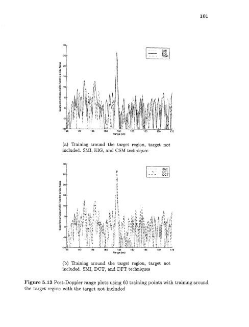
Page 114 and 115: 99(a) Training outside the target r
Page 118 and 119: 103Figure 5.15 Angle scan with the
Page 120 and 121: CHAPTER 6CONCLUSIONSThis work has b
Page 122 and 123: 107also presented. The Sample Matri
Page 124 and 125: APPENDIX ADISCRETE COSINE TRANSFORM
Page 126 and 127: 111This matrix is formed using the
Page 128 and 129: REFERENCES1. Leon Cohen. Time-frequ
Page 130 and 131: 11523. Franz Hlawatsch and G. Faye
Page 132 and 133: 11750. Daniel F. Marshall. A two st
Page 134 and 135: INDEXanalytic signal, 21array imper
show all

Space/time/frequency methods in adaptive radar - New Jersey ...

You also want an ePaper? Increase the reach of your titles

Delete template?

Save as template?