Simulation of a Vacuum-Tube Push-Pull Guitar Power Amplifier

More documents

Recommendations

Info

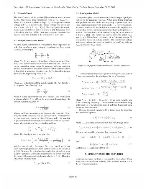
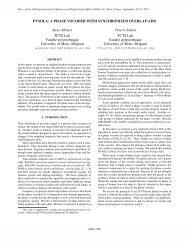
Proc. of the 14 th Int. Conference on Digital Audio Effects (DAFx-11), Paris, France, September 19-23, 2011Proc. of the 14th International Conference on Digital Audio Effects (DAFx-11), Paris, France, September 19-23, 20112.1. Pentode ModelThe Koren’s model of the pentode [7] was chosen as the pentodemodel. The pentode plate current is in form I a(V ak , V gk1 , V gk2 )where V ak is plate-to-cathode voltage, V g1k is the grid-to-cathodevoltage and U g2k is the screen-to-cathode voltage. The screen currentis given in form I s(V gk1 , V gk2 ). The description of functionsI a and I s is omitted here and is available in [7]. Frequency propertiesof the tube (e.g. Miller capacitance) are not considered becauseit should be included in the simulation of input unit.2.2. Output Transformer ModelAn ideal output transformer is considered to be an impedance dividerthat transforms input voltages V p and currents I p to outputV s and I s according to2.3. Loudspeaker ModelLoudspeakers play a very important role in the output signal generationvia its frequency response. When considering linearizedloudspeakers, one can model the frequency response with measuredimpulse responses with good results [1]. However, it is importantto simulate the interaction between the tube amplifier andloudspeaker because the loudspeaker impedance is frequency dependent.The impedance can be modeled using the circuit schematicin figure 2 [12]. The values are derived from the added massmethod and Thiele/Small parameters of a Celestion Vintage 30loudspeaker placed in an Engl combo. The transformer leakageinductance and resistance can be modeled by modifying inductorL sp1 and resistor R sp1 values.V sV p= N2N 1= IpI s(1)where N 1, N 2 are numbers of windings of the transformer. However,a real transformer is far away from the ideal one. For an accuratesimulation, losses caused by hysteresis and core saturationhave to be considered. Nonlinear behavior of the real transformeris described in numerous literature, e.g. [8, 9]. According to Amper’slaw, the magnetizing force H isHl mag = N 1I p − N 2I s (2)where l mag is the length of the induction path. The flux density Bis computed from Farraday’s law∂B∂t =Vs(3)N 2Swhere S is the transformer-core cross-section. The well-knownnonlinear relation B = µH can be implemented according to theFrolich equation [9] given byB =Hc + b |H|where c and b are constants derived from material properties. However,this model simulates only the core saturation. When simulatinghysteresis, one can use e.g. Jiles-Atherton model [10] modifiedin [8] in order to remove nonphysical behavior of minor hysteresisloops. Magnetization of the core is obtained from∂M∂H = M an − MδM + c ∂Mankδ ∂Hwhere M an is anhysteretic curve given by( H + αMM an = M s(cotha)−)aH + αMand δ =sign(∂H/∂t). Parameters M s, α, a, c and k are derivedfrom material properties and their identification can be found e.g.in [11]. Parameter δ M =0when the nonphysical minor loop is goingto be generated (anhysteric magnezation has lower value thanthe irreversible magnezation) alternatively δ M =1[8] . Flux densityis then obtained from(4)(5)(6)B = µ 0 (M + H) . (7)Figure 2: Simplified loudspeaker model – electric equivalent.The loudspeaker impedance given by voltage V L and currentI L can be expressed as the solution of the set of equationsVL[n] − IL[n]Rsp1 − V3[n]I L[n] =I L[n − 1] +L sp1f sV3[n]Gsp2 − IL[n] − IL2[n]V 3[n] =V 3[n − 1] + (8)C sp1f sI L2[n] =I L2[n − 1] + V3[n]L sp2f swhere I L[n − 1], V 3[n − 1], I L2[n − 1] are state variables andf s is a sampling frequency. The equations were obtained usingnodal analysis of the circuit in figure 2 and then discretized usingBackward Euler formula.Because the set of equations (8) is linear, it can be simplifiedinto one linear equationI L[n] =−c 1V L[n]+I tmp (9)where I tmp is a linear combination of state variables given byI tmp = −c 2I L[n − 1] + c 3V 3[n − 1] − c 4I L2[n − 1]. (10)The new state variable values are then computed fromV 3[n] =−c 5V 3[n − 1] − c 6I L[n]+c 7I L2[n − 1] (11)andI L2[n] =I L2[n − 1] + c 8V 3[n]. (12)Coefficients c 1−8 are derived from (8).3. SIMULATION OF THE AMPLIFIERIn the simplest case, the load is considered to be constant. Usingnodal analysis and discretization by Euler method, one can obtainthe set of circuit equationsDAFX-2DAFx-60
Proc. of the 14 th Int. Conference on Digital Audio Effects (DAFx-11), Paris, France, September 19-23, 2011Proc. of the 14th International Conference on Digital Audio Effects (DAFx-11), Paris, France, September 19-23, 20114. SIMULATION RESULTS0=− VL[n] + N1(I a1 − I a2)R L N 20=−V a1[n]+V D[n] − N1V L[n]N 20=−V a2[n]+V D[n]+ N1V L[n]N 2VD[n] − Vs1[n]0=I s1 +0=I s2 +R s1VD[n] − Vs2[n]R s2,(13)where V D is voltage on the power supply, capacitor C d is from thecircuit schematic in figure 1 and I a1 = I a(V in1[n],V a1[n],V s1[n]),I s = I s (V in1[n],V s1[n]) and similarly I s2 = I s (V in2[n],V s2[n])and I a2 = I a(V in2[n],V a2[n],V s2[n]). The equations (13) aresolvable for given value V D and the solution can be implementedusing a static waveshaper. It can be precomputed for different valuesof V D voltage and stored in a look-up table. Then, during thesimulation, the proper static waveshaper is chosen according to theV D voltage. The V D voltage is then actualized usingV D[n] = −Ia1 − Ia2 − Is1 − Is2 + (V PS−V D [n−1 ])R D+ V D[n − 1].C 1f fs(14)3.1. Circuit with Loudspeaker ModelIf the loudspeaker is connected to the power amplifier, the loadimpedance is no longer given explicitly, but it is determined by V L,I L relation implicitly given by equations (8). In order to excludethe loudspeaker impedance R L, the first equation from system (13)is modified toI L[n] = N1(I a1 − I a2) (15)N 2and then solution of the modified equations (13) with (15) is expressedas a function I L[n] =f IL (V in1[n],V in2[n],V D[n],V L[n]).Finally, the solution of the whole system using (9) is given by− c 1V L[n]+I tmp = f IL (16)for the unknown variable V L[n] and state variables I tmp and V D[n].3.2. Circuit with Nonlinear Transformer ModelThe simulation of a circuit with a nonlinear transformer model isbased on (2), (3) and the nonlinear core model. The system isdescribed using0=−H(B[n])l mag − (c 1V L[n]+I tmp)N 2 + f ILN 20=B[n − 1] − B[n]+VL(17)N 2Sf swhere term f ILN 2 is recomputed current I L to primary winding,B[n − 1] is the flux density in the previous sampling period andH(B) is the core model derived from (4) or from (7) if the hysteresisis considered.All the simulations from section 3 were implemented in Matlabenvironment using Mex files and C language. The Newton methodwas used for solving implicit nonlinear equations. The derivationof function or the Jacobian matrix were obtained using finite differenceformula, the maximal number of iterations was 100 and thenumerical error was chosen as 0.0001. The values for the transformermodel were chosen experimentally: M s = 1.11 × 10 6 ,3a =8.56, α =8.82×10 −5 , c =0.14 and k =51.65. However,they can be computed from a measured hysteresis loop data [11].The parameters for the Frohlich core model were c = 113.38,b =0.71 and the dimensions of the transformer were chosen asS =0.003 m 2 and l mag =0.2 m.The transformer-core cross-section S together with the numberof windings determines the low cutoff frequency of the transformer.The simulation of the output part of the power amplifierwas appended with a phase splitter, input pentode unit and feedbackaccording to [1] and the results were compared to the measuredEngl combo. The data was obtained from a measured voltageon a parallel loudspeaker output with connected soundcard. Thefrequency dependence of the first harmonic content of the voltageoutput signal, obtained using sweep sine signal, is shown infigure 3. The simulation with a constant load provides the worstresults – there is no resonance around 45 Hz that appears in allof the other simulations and measured data. The simulation withhysteresis loop has similar behavior as a measured amplifier in thearea of low frequencies due to the core losses. In the area of midfrequencies,the simulation and measured data differ because ofthe other resonances and mechanical properties of the loudspeakerdiaphragm, which are not considered in the simulation but can beincluded in the simulation by improving the loudspeaker modellike in [13]. The nonlinear distortion was investigated as well. Theoutput spectrum for an input sinewave signal with an amplitude of2 V is shown in figures 4. The individual spectra are measured forthe same frequency but they are shifted in the graph. All the algorithmsexcluding the variant with constant load give very similarresults. The nonlinear distortion caused by transformer hysteresismanifests very slightly and only at frequencies below cca 150 Hzand it is very dependent on transformer parameters. The spectrogramof simulation using JA-model is shown in figure 5.The table 2 shows the hypothetical computational complexitythat was determined using measurement of time duration of simulationfor input guitar riff signal with a length of 18 s and an amplitudeof 30 V. The results showed that the algorithm is capable ofworking in real-time. Sound examples of all the algorithm variantsand detailed graphs and other spectrograms are available on theweb page www.utko.feec.vutbr.cz/~macak/DAFx11/.Table 2: Normalized computational complexity.Constant load Loudspeaker Frohlich J-A model0.04 % 0.05 % 0.12 % 0.27 %5. CONCLUSIONSThe simulation of a push-pull tube amplifier was discussed in thispaper. The impact of the loudspeaker and output transformer toDAFX-3DAFx-61
Page 1: Proc. of the 14 th Int. Conference

Simulation of a Vacuum-Tube Push-Pull Guitar Power Amplifier

Create successful ePaper yourself

Delete template?

Save as template?