EXPONENTIAL FREQUENCY MODULATION BANDWIDTH ...

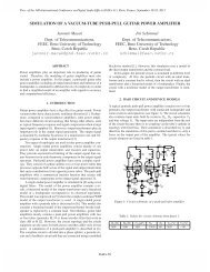
Proc. of the 14th International Conference on Digital Audio Effects (DAFx-11), Paris, France, September 19-23, 2011Proc. of the 14 th Int. Conference on Digital Audio Effects (DAFx-11), Paris, France, September 19-23, 2011EXPONENTIAL FREQUENCY MODULATION BANDWIDTH CRITERION FOR VIRTUALANALOG APPLICATIONSJoseph Timoney, Victor Lazzarini,Sound and Music Technology ResearchGroup, NUI MaynoothMaynooth, Irelandjtimoney@cs.nuim.ievictor.lazzarini@nuim.ieABSTRACTCross modulation or Exponential FM is a sound synthesis techniqueassociated with modular analog subtractive synthesizers. Itdiffers from the more well-known linear FM synthesis techniquein that the modulation is an exponential function of the controlvoltage. Its spectrum shape is more complex, thus giving it a largerbandwidth with respect to the modulation depth. Thus, theprevention of aliasing distortion requires different conditionsthan Carson’s rule as used with linear FM. A suitable equationwill be presented in this paper.1. INTRODUCTIONResearch into virtual implementations of the structures of analogsubtractive synthesizers has been a popular topic for the last fewyears. There have been a number of algorithms proposed to createbandlimited versions of the classic analog oscillators [1].Alongside this, there have been a number of papers that derivemodels for the Voltage controlled filters associated with particularanalog synthesizers. The designs for these have been based onan explicit circuit analysis, [2] for example, or those that create aversion of the original using standard digital filter elements [3].However, other elements of subtractive synthesis systems havenot received such in-depth treatment such as the Attack-Decay-Sustain-Release (ADSR) envelope generators, Filter FM effects,and other oscillator modulation configurations. Although onmodern analog synthesizers linear Frequency modulation (FM)between oscillators is sometimes a feature this was not alwaysthat case. In fact, Linear Frequency Modulation is really associatedwith digital synthesis and was viewed as the synthesis technologythat overtook subtractive synthesis in the 1980s [4]. LinearFrequency modulation was unavailable in early modular subtractivesynthesis systems for two primary reasons: Firstly, it wasdifficult to implement because of the Volts/Octave control voltageconcept on which the elements of these synthesizers wereinterconnected. This system creates a non-linear relationship betweenany change in signal voltage and the pitch [5]. Thus, toforce it to behave in a linear manner was difficult. Secondly, thetuning instabilities associated with early analog synthesizers becauseof component drift and ambient temperature fluctuationswould have resulted in inconsistent generation of stable linearFM signals [6]. This is particular important in the case when thelinear FM signal is desired to be harmonic; to achieve this, thefrequencies of the carrier and modulator signals must strictly bein an integer relationship. Any deviation from this can seriouslyaffect the perception of the sound.The nonlinear Volts/Octave control voltage relationship of theseanalog synthesizers meant that modulation of one oscillator byanother actually produced an Exponential FM waveform. Onenotable feature of this technique was that when the modulationdepth was varied dynamically, a pitch shifting of the sound wasperceived. This issue meant that for musicians Exponential FMwas most often used to produce special effect sounds that wereclangorous rather than for melodic lines. An excellent treatmentof the theory of Exponential FM was written by [7]. This paperprovided a description of the signal and its spectrum for sinewavemodulators. It also offered a configuration of analog modulesthat introduced a pitch correction factor that could be usedto produce a harmonic version of Exponential FM. However, thework in [7] was written for implementation on an analog synthesizersystem and thus assumed an infinite output bandwidth. Thisis not the case for digital implementations and algorithm designersalways have to be aware of limitations on signal bandwidthimposed by the sampling frequency so as to minimise aliasingdistortion. Therefore, this paper will examine the implementationof Exponential FM from a digital perspective. It will examine thespectra produced by the Exponential FM system in an effort toproduce a guideline for its digital implementation. Section 2 willintroduce the theory behind Exponential FM and will provide thespectral bandwidth analysis. Section 3 will contain the conclusions.2. THEORY OF EXPONENTIAL FMFirst of all, the Volts/Octave control signal representation in analogsynthesizers means that the pitch of a note doubles as thecontrol voltage doubles [5]. Thus, the relationship can be expressedVf ∝ 2(1)where f is the note pitch and V is the control voltage.For example, if 2 volts produces a pitch of 110Hz, then 3 voltswill produce a note an octave higher of 220Hz.Next, although the well-known equation for linear FMsynthesis is actually phase modulation, on a modular synthesizersystem Exponential FM is implemented as a true frequencymodulation. The modulator signal voltage is interpreted as frequencyvariation that is used to define the control voltage associatedwith frequency of the carrier. The modulator is thus an instantaneousfrequency signal that for exponential FM is definedas in [7] to beDAFX-1DAFx-115

Proc. of the 14th International Conference on Digital Audio Effects (DAFx-11), Paris, France, September 19-23, 2011Proc. of the 14 th Int. Conference on Digital Audio Effects (DAFx-11), Paris, France, September 19-23, 2011V ( t )( t) = 2θ & (2)where f c and f m are the Carrier and Modulation frequencies inhertz respectively, and V(t) represents the modulating signal.Note that the dot on the term on the left hand side indicates thatit is a differential (of the phase).The Modulating signal can be written as the combinationof a DC term, V 0 and a time-varying quantity, assumed to bea cosine here, of amplitude V m, , which can also be termed as theModulation Depth [7],V t = V + V cos 2πft(3)f c( ) ( )0Substituting (3) into (2) and using logarithms to write the powertermwhich can be rewrittenmV0 + Vmcos ( 2πfmt)( t) = f em( ) ln ( 2)cθ & (4)The expression in (10) is a multi-component complex FM signal.2.1. Carrier Frequency AnalysisFrom (6) and (10) it can be seen that the final carrier frequencyof the Exponential FM signal is a function of the exponent of theDC term V 0 and the value of the zero th modified Bessel functionthat has the Modulation Depth in its argument. This is differentto the linear FM case where the carrier frequency is independentof the modulation. This relationship should be taken into accountfor the digital version of Exponential FM. For example, assumingfor convenience that the DC term V 0 is zero it is possible toshow graphically how the carrier frequency increases with increasingmodulation amplitude. This is illustrated in Figure 1where the input carrier frequency f c is plotted along the x-axis,the Modulation Depth V m on the y-axis, and the actual carrierfrequency given by (11) on the z-axis. The maximum possiblevalue of the input carrier was assumed to be 8372Hz, correspondingto midi-note #120.withVmcos ( 2πfmt)( t) = f e( ) ln ( 2)θ & (5)ceV ln ( 2 0 )fce= fce(6)To convert the instantaneous frequency signal into a phase theexponential term in (5) must be integrated( ) = ∫ θ ( t )θ t & (7)However, it is not possible to integrate the exponential term in(5) directly and instead it must be expanded as set of ModifiedBessel functions [7]( 2πfmt) ln( 2) = I ( V ln( 2)) + 2 I ( V ln( 2)) cos( 2πkft)0m∑ ∞ kk = 1Vm cose(8)Substituting (8) back into (5)& ⎛⎞( t) = I0( Vmln( 2)) fce+ ⎜2Ik( Vmln( 2)) cos( 2πkfmt) ⎟ f(9)c⎝⎠θ ∑ ∞k=1Integrating to obtain the phase as shown by (7) and assuming asinusoidal carrier will produce the time domain signal [7]⎛⎛=⎜⎜∑ ∞ 2 fmce⎝⎝ k=1kf( ) ( ( )) ⎜ct sin θ t = sin 2πI( V ln( 2)) f t + ⎜ I ( V ln( 2)) sin( πkft) ⎟⎟ym0 k m2mThe carrier frequency of (11) can be written asE( V mln( )) f ceand the frequency deviation of each term ism⎞⎞m ⎟⎠⎠(10)f = I 2(11)02 fcDk= Ikfmk( V ln( 2))m(12)Figure 1: The relationship between the input carrier frequency,the modulation depth and the actual carrier frequency.From Figure 1 it can be seen the actual carrier frequency increasesquite rapidly as the Modulation Depth V m reaches valuesof 8 or more. This illustrates the difference between linear FMand Exponential FM well. It also hints at the problems that canoccur with the digital implementation of Exponential FM andwarns that care must be taken when setting a sampling frequencyfor any implementation so that it is commensurate with the widthof the Modulation Depth control. Lastly, looking at (11) it can beseen that including a DC term (V 0 ) in the modulating signal addsfurther complications in that it can raise the carrier frequencysignificantly. For example, for V 0 =5 the carrier frequency will bescaled by a factor of 7.17.2.2. Computing the Spectrum of Exponential FMTo obtain the spectrum of the Exponential FM signal in (10)there are a number of possible approaches. These can be numerical,analytical, or a hybrid of the two. Note though what is moreuseful here is the spectrum envelope rather than the actual spectrumitself. When attempting to compute the bandwidth it ismuch easier to work with the envelope because any gaps that existbetween the partials in the signal that can disrupt an auto-DAFX-2DAFx-116

Proc. of the 14th International Conference on Digital Audio Effects (DAFx-11), Paris, France, September 19-23, 2011Proc. of the 14 th Int. Conference on Digital Audio Effects (DAFx-11), Paris, France, September 19-23, 2011mated spectral analysis process to find a significant low energyspectral region.The most obvious numerical technique to use is theFast Fourier Transform (FFT). This is readily available in mostsoftware environments. However, this does not produce the envelopeitself and further processing is required for this. Methods toachieve this include autoregressive analysis or Cepstral techniques.Another approach is to employ the semi-analyticmethod of [8] that expresses the frequency modulation itself as apiecewise linear function. The total spectrum of the modulatedoutput is the summation of the spectra for each piecewise-linearmodulated part of the entire waveform. In essence this modelsthe modulated waveform as a succession of linear Chirp signals,and thus the spectrum is the combination of the spectra for thesechirps. In [8] it is proposed that the spectrum of the chirp signalis obtained using a numerical evaluation of the Fresnel equations.A faster estimate can be obtained using a Stationary Phase Approximation(SPA) and it also does not have any associated numericalintegration issues [9]. However, efforts to apply thistechnique were not successful. It resulted in an approximatespectrum that had a blocky appearance which was not a particularlygood match to the FFT based spectrum. It neither capturedthe true height of the various spectral components or the completewidth of the spectrum.Aside from the quasi-static approach for spectral approximationthat is allowable under very particular conditions[10], the most general analytical approach is to expand the modulationterm of (10) using Bessel functions [10]. Rewriting (10) bysubstituting (11) and (12)It can be expanded as [10]⎛sin⎜ωn+⎝k∑D sin⎛ ⎛=⎜ ∑ ∞ E⎝ ⎝ k=1⎞⎞( t) sin⎜2πft + ⎜ D sin( 2πkft) ⎟ ⎟ y⎞⎛km⎠⎠( ω ) ∑ ∑ ∏ ( ) ⎜kn+ ϕk⎟ = K ⎜ JkDk⎟sinωn+ ⎜∑ki( ωin+ ϕi)iki = 1k k k1 i = 1i = 1⎠⎝k⎞⎠⎛⎜⎝⎛⎝k(13)(14)An example of using (14) to produce the magnitude spectrum isgiven in Figure 2 for f c =440Hz and f m =44Hz and V m =2. In thefigure the reflection of the negative frequencies back into thepositive frequency region was not carried out as these always introducespectral zeros for this particular signal case, while whatis required is a smooth spectral envelope. It can be seen in Figure2 that the envelope has a number of resonant peaks that becomewider with respect to increasing frequency. The most significantcomponent is below about half the carrier frequency. Althoughthe higher frequency components are smaller than the carrier thespectrum does not have a true lowpass shape, but rather curvesupwards at the last resonant peak.⎞⎟ ⎞⎟⎠⎠Magnitude0.40.350.30.250.20.150.10.05Magnitude Spectrum computed analytically using Bessel Functions00 500 1000 1500 2000 2500Frequency (Hz)Figure 2: Magnitude spectrum of an Exponential FM signal usinga Bessel Function Analysis.There are two difficulties with the Bessel function based spectralanalysis. Firstly, given that (14) is a complicated expression involvingproduct terms, it is only possible to evaluate it numerically.This means that it cannot provide an intuitive compact expression.Secondly, the complexity of the evaluation of the equationgrows exponentially with each additional sinusoidal term inthe modulation signal. Some savings can be made by eliminatingthe evaluation of low amplitude Bessel function terms from thecomputation, and using programming optimisations to avoid thenested loop implementation.2.3. Spectral Bandwidth EvaluationThe spectral bandwidth such that aliasing components would beof sufficiently low magnitude was defined to be point at whichthe spectrum was 80dB below the peak value. This was a reasonablystrict criteria and much stronger than Carson’s rule [10].The intention was to express the Bandwidth as a function of thecarrier frequency and the Modulation Depth.First, using (14) the spectra of Exponential FM signalswere computed for different values of carrier frequency and withfixed values for the modulation frequency and modulation depth.It was found that under these conditions the spectra were simplytranslated in relation to the carrier meaning shape invariant to thecarrier frequency.Next, spectra were again generated with the modulationfrequency was expressed as a ratio of the carrier frequency from0.1 up to 1 for a fixed value of Modulation Depth, and the bandwidthmeasured by an automated analysis in each case. This wasrepeated for other values of Modulation Depth. Figure 3 shows aplot of the results for values of Modulation Depth V m, =1, 2 and 3.The Bandwidth relative to the carrier frequency is shown on they-axis as a multiple of the carrier frequency. From the plot it canbe seen that the relationship between the Modulation frequencyand relative Bandwidth is almost linear for all values of V m, .Thus, a simple linear fit can be made to characterize the relationship.DAFX-3DAFx-117

Proc. of the 14th International Conference on Digital Audio Effects (DAFx-11), Paris, France, September 19-23, 2011Proc. of the 14 th Int. Conference on Digital Audio Effects (DAFx-11), Paris, France, September 19-23, 201118Spectral Bandwith relative to the modulation frequency0V0=1 Vm=4 fm/fc=2.5Bandwidth in multiples of the input carrier frequency16141210864Vm=1Vm=2Vm=3Magnitude dBMagnitude dB-20-40-60-800 1000 2000 3000 4000 5000 6000 7000Frequency (Hz)V0=0 Vm=7 fm/fc=40-20-40-60-800.1 0.2 0.3 0.4 0.5 0.6 0.7 0.8 0.9 1Modulation frequency as a ratio of the carrier frequency (fm/fc)Figure 3: Spectral Bandwidth shown as a function of the Modulationfrequency expressed as a ratio of the carrier frequency forthree different values of Modulation Depth.For the three different values of V m in the figure the coefficientscalculated are given in Table 10 500 1000 1500 2000Frequency (Hz)Figure 4: Example plots of FFT spectra of Exponential FMsignals with the -80dB Bandwidth in Hz highlighted usinga dashed line in both panels. Upper panel parameterswere f c =100Hz and f m =250Hz, V 0 =1 and V m =4 and for thelower panel were f c =10Hz and f m =40Hz, V 0 =0 and V m =7.V m p 0 p 11 2.771 4.30302 5.168 6.46063 9.3841 9.2485Table 1: Coefficients linear fit to data in Figure 4 for differentvalues of Modulation Depth.The equation for the relative Bandwidth (to be multiplied by f cfor the value in Hz) was( f , f , V ) p + p ( f f )BWc m m 0 1= (15)To create a more general expression that also includes V m on theright hand side of (15) the values in Table I can be examined. Itcan be seen that as V m increases the value for p 1 increases approximatelyby a factor V m . Similarly, the value for p 0 increasesby about V m -1 to the power of 2. Incorporating this along withpossible scaling of f c by the DC term V 0 , (15) gives the final expressionfor the -80dB bandwidth in HertzV ( ) V( fcfm) = fceln 2 −1p01+ ( p V m) f m0 mBW , + (16)−80dBHz211where p = 012. 771 and p11= 4. 3030.Two examples are given in Figure 4 to illustrate the validity ofthis expression. These are shown in Figure 4. In the upper panelthe values to generate the Exponential FM signal were f c =100Hzand f m =250Hz, V 0 =1 and V m =4. Its actual spectrum was computedusing a Hanning windowed FFT and is displayed using adB scale. The equation in (16) was used to find the bandwidth inHz. This is plotted using the dashed vertical line in the figure. Itclearly marks a point close to -80dB in front of the primary spectralregion. In the lower panel the values were f c =10Hz andf m =40Hz, V 0 =0 and V m =7. Again, the dB magnitude FFT wasfound and the bandwidth was plotted using a dashed vertical line.In this case it actually estimates the -80dB to be at a greater locationin frequency. However, this error is acceptable as it is anoverestimation rather than an underestimation.mc3. CONCLUSIONSThis paper has presented an expression to evaluate the -80dBbandwidth of a cosine modulated Exponential FM signal. Exampleswere given to demonstrate its effectiveness. It should be auseful formula for low-aliasing digital implementations of ExponentialFM. Future work aims to produce an exact analytical expressionfor the spectrum of the Exponential FM signal. It willalso investigate bandwidth criteria for cases when the modulationis not sinusoidal, such as for sawtooth and square waves.4. REFERENCES[1] Välimäki, V., and A. Huovilainen 2007, ‘Antialiasing oscillatorsin subtractive synthesis,’ IEEE Signal ProcessingMagazine, 24(2): 116–125.[2] M. Civolani and F. Fontana, 'A nonlinear digital model ofthe EMS VCS3 voltage controlled filter', Proc. Dafx 2008,Espoo, Finland, Sept. 2008.[3] V. Välimäki and A. Huovilainen, ‘Oscillator and filter algorithmsfor virtual analog synthesis’ Computer Music Journal,vol. 30, no. 2, pp. 19-31, 2006.[4] J. Chowning and D. Bristow, FM theory and applications –By Musicians for musicians, Yamaha, Tokyo, Japan, 1986.[5] H. Chamberlain, H., Musical Applications of Microprocessors,Hayden Books, Indianapolis, Indiana, USA, 1987.[6] M. Russ, Sound synthesis and sampling, Focal press, Elsevier,Oxford, UK, 2009.[7] B. Hutchins, ‘The frequency modulation spectrum of an exponentialvoltage-controlled oscillator,’ Jnl. Of Audio Eng.Soc., Vol. 23(3), April 1975, pp. 200-206.[8] J. Martin, A. Holt and G. Salkeld, ‘Novel analytic techniquefor obtaining the spectrum associated with piecewise linearFM,’ Proc. IEE, Vol. 122(7), Jul. 1975, pp. 710-712.[9] E. Chassande-motin and P. Flandrin, 'On the stationaryphase approximation of chirp spectra', Proc. IEEE TFTS1998, Pittsburg, PA, USA, Oct. 1998.[10] H. Rowe, Signals and noise in communications systems,Van Nostrand, NJ, USA, 1965.DAFX-4DAFx-118