EXPONENTIAL FREQUENCY MODULATION BANDWIDTH ...

More documents

Recommendations

Info

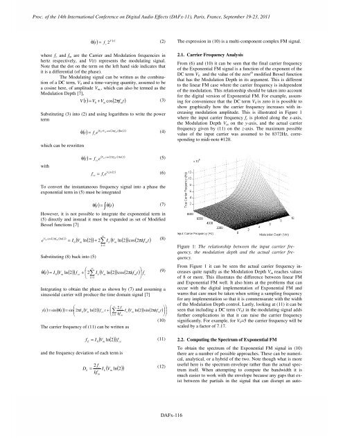
Proc. of the 14th International Conference on Digital Audio Effects (DAFx-11), Paris, France, September 19-23, 2011Proc. of the 14 th Int. Conference on Digital Audio Effects (DAFx-11), Paris, France, September 19-23, 2011V ( t )( t) = 2θ & (2)where f c and f m are the Carrier and Modulation frequencies inhertz respectively, and V(t) represents the modulating signal.Note that the dot on the term on the left hand side indicates thatit is a differential (of the phase).The Modulating signal can be written as the combinationof a DC term, V 0 and a time-varying quantity, assumed to bea cosine here, of amplitude V m, , which can also be termed as theModulation Depth [7],V t = V + V cos 2πft(3)f c( ) ( )0Substituting (3) into (2) and using logarithms to write the powertermwhich can be rewrittenmV0 + Vmcos ( 2πfmt)( t) = f em( ) ln ( 2)cθ & (4)The expression in (10) is a multi-component complex FM signal.2.1. Carrier Frequency AnalysisFrom (6) and (10) it can be seen that the final carrier frequencyof the Exponential FM signal is a function of the exponent of theDC term V 0 and the value of the zero th modified Bessel functionthat has the Modulation Depth in its argument. This is differentto the linear FM case where the carrier frequency is independentof the modulation. This relationship should be taken into accountfor the digital version of Exponential FM. For example, assumingfor convenience that the DC term V 0 is zero it is possible toshow graphically how the carrier frequency increases with increasingmodulation amplitude. This is illustrated in Figure 1where the input carrier frequency f c is plotted along the x-axis,the Modulation Depth V m on the y-axis, and the actual carrierfrequency given by (11) on the z-axis. The maximum possiblevalue of the input carrier was assumed to be 8372Hz, correspondingto midi-note #120.withVmcos ( 2πfmt)( t) = f e( ) ln ( 2)θ & (5)ceV ln ( 2 0 )fce= fce(6)To convert the instantaneous frequency signal into a phase theexponential term in (5) must be integrated( ) = ∫ θ ( t )θ t & (7)However, it is not possible to integrate the exponential term in(5) directly and instead it must be expanded as set of ModifiedBessel functions [7]( 2πfmt) ln( 2) = I ( V ln( 2)) + 2 I ( V ln( 2)) cos( 2πkft)0m∑ ∞ kk = 1Vm cose(8)Substituting (8) back into (5)& ⎛⎞( t) = I0( Vmln( 2)) fce+ ⎜2Ik( Vmln( 2)) cos( 2πkfmt) ⎟ f(9)c⎝⎠θ ∑ ∞k=1Integrating to obtain the phase as shown by (7) and assuming asinusoidal carrier will produce the time domain signal [7]⎛⎛=⎜⎜∑ ∞ 2 fmce⎝⎝ k=1kf( ) ( ( )) ⎜ct sin θ t = sin 2πI( V ln( 2)) f t + ⎜ I ( V ln( 2)) sin( πkft) ⎟⎟ym0 k m2mThe carrier frequency of (11) can be written asE( V mln( )) f ceand the frequency deviation of each term ism⎞⎞m ⎟⎠⎠(10)f = I 2(11)02 fcDk= Ikfmk( V ln( 2))m(12)Figure 1: The relationship between the input carrier frequency,the modulation depth and the actual carrier frequency.From Figure 1 it can be seen the actual carrier frequency increasesquite rapidly as the Modulation Depth V m reaches valuesof 8 or more. This illustrates the difference between linear FMand Exponential FM well. It also hints at the problems that canoccur with the digital implementation of Exponential FM andwarns that care must be taken when setting a sampling frequencyfor any implementation so that it is commensurate with the widthof the Modulation Depth control. Lastly, looking at (11) it can beseen that including a DC term (V 0 ) in the modulating signal addsfurther complications in that it can raise the carrier frequencysignificantly. For example, for V 0 =5 the carrier frequency will bescaled by a factor of 7.17.2.2. Computing the Spectrum of Exponential FMTo obtain the spectrum of the Exponential FM signal in (10)there are a number of possible approaches. These can be numerical,analytical, or a hybrid of the two. Note though what is moreuseful here is the spectrum envelope rather than the actual spectrumitself. When attempting to compute the bandwidth it ismuch easier to work with the envelope because any gaps that existbetween the partials in the signal that can disrupt an auto-DAFX-2DAFx-116
Proc. of the 14th International Conference on Digital Audio Effects (DAFx-11), Paris, France, September 19-23, 2011Proc. of the 14 th Int. Conference on Digital Audio Effects (DAFx-11), Paris, France, September 19-23, 2011mated spectral analysis process to find a significant low energyspectral region.The most obvious numerical technique to use is theFast Fourier Transform (FFT). This is readily available in mostsoftware environments. However, this does not produce the envelopeitself and further processing is required for this. Methods toachieve this include autoregressive analysis or Cepstral techniques.Another approach is to employ the semi-analyticmethod of [8] that expresses the frequency modulation itself as apiecewise linear function. The total spectrum of the modulatedoutput is the summation of the spectra for each piecewise-linearmodulated part of the entire waveform. In essence this modelsthe modulated waveform as a succession of linear Chirp signals,and thus the spectrum is the combination of the spectra for thesechirps. In [8] it is proposed that the spectrum of the chirp signalis obtained using a numerical evaluation of the Fresnel equations.A faster estimate can be obtained using a Stationary Phase Approximation(SPA) and it also does not have any associated numericalintegration issues [9]. However, efforts to apply thistechnique were not successful. It resulted in an approximatespectrum that had a blocky appearance which was not a particularlygood match to the FFT based spectrum. It neither capturedthe true height of the various spectral components or the completewidth of the spectrum.Aside from the quasi-static approach for spectral approximationthat is allowable under very particular conditions[10], the most general analytical approach is to expand the modulationterm of (10) using Bessel functions [10]. Rewriting (10) bysubstituting (11) and (12)It can be expanded as [10]⎛sin⎜ωn+⎝k∑D sin⎛ ⎛=⎜ ∑ ∞ E⎝ ⎝ k=1⎞⎞( t) sin⎜2πft + ⎜ D sin( 2πkft) ⎟ ⎟ y⎞⎛km⎠⎠( ω ) ∑ ∑ ∏ ( ) ⎜kn+ ϕk⎟ = K ⎜ JkDk⎟sinωn+ ⎜∑ki( ωin+ ϕi)iki = 1k k k1 i = 1i = 1⎠⎝k⎞⎠⎛⎜⎝⎛⎝k(13)(14)An example of using (14) to produce the magnitude spectrum isgiven in Figure 2 for f c =440Hz and f m =44Hz and V m =2. In thefigure the reflection of the negative frequencies back into thepositive frequency region was not carried out as these always introducespectral zeros for this particular signal case, while whatis required is a smooth spectral envelope. It can be seen in Figure2 that the envelope has a number of resonant peaks that becomewider with respect to increasing frequency. The most significantcomponent is below about half the carrier frequency. Althoughthe higher frequency components are smaller than the carrier thespectrum does not have a true lowpass shape, but rather curvesupwards at the last resonant peak.⎞⎟ ⎞⎟⎠⎠Magnitude0.40.350.30.250.20.150.10.05Magnitude Spectrum computed analytically using Bessel Functions00 500 1000 1500 2000 2500Frequency (Hz)Figure 2: Magnitude spectrum of an Exponential FM signal usinga Bessel Function Analysis.There are two difficulties with the Bessel function based spectralanalysis. Firstly, given that (14) is a complicated expression involvingproduct terms, it is only possible to evaluate it numerically.This means that it cannot provide an intuitive compact expression.Secondly, the complexity of the evaluation of the equationgrows exponentially with each additional sinusoidal term inthe modulation signal. Some savings can be made by eliminatingthe evaluation of low amplitude Bessel function terms from thecomputation, and using programming optimisations to avoid thenested loop implementation.2.3. Spectral Bandwidth EvaluationThe spectral bandwidth such that aliasing components would beof sufficiently low magnitude was defined to be point at whichthe spectrum was 80dB below the peak value. This was a reasonablystrict criteria and much stronger than Carson’s rule [10].The intention was to express the Bandwidth as a function of thecarrier frequency and the Modulation Depth.First, using (14) the spectra of Exponential FM signalswere computed for different values of carrier frequency and withfixed values for the modulation frequency and modulation depth.It was found that under these conditions the spectra were simplytranslated in relation to the carrier meaning shape invariant to thecarrier frequency.Next, spectra were again generated with the modulationfrequency was expressed as a ratio of the carrier frequency from0.1 up to 1 for a fixed value of Modulation Depth, and the bandwidthmeasured by an automated analysis in each case. This wasrepeated for other values of Modulation Depth. Figure 3 shows aplot of the results for values of Modulation Depth V m, =1, 2 and 3.The Bandwidth relative to the carrier frequency is shown on they-axis as a multiple of the carrier frequency. From the plot it canbe seen that the relationship between the Modulation frequencyand relative Bandwidth is almost linear for all values of V m, .Thus, a simple linear fit can be made to characterize the relationship.DAFX-3DAFx-117
Page 1: Proc. of the 14th International Con

EXPONENTIAL FREQUENCY MODULATION BANDWIDTH ...

Create successful ePaper yourself

Delete template?

Save as template?