EXPONENTIAL FREQUENCY MODULATION BANDWIDTH ...

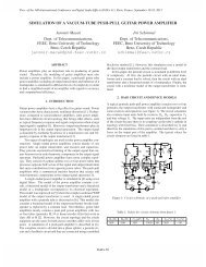
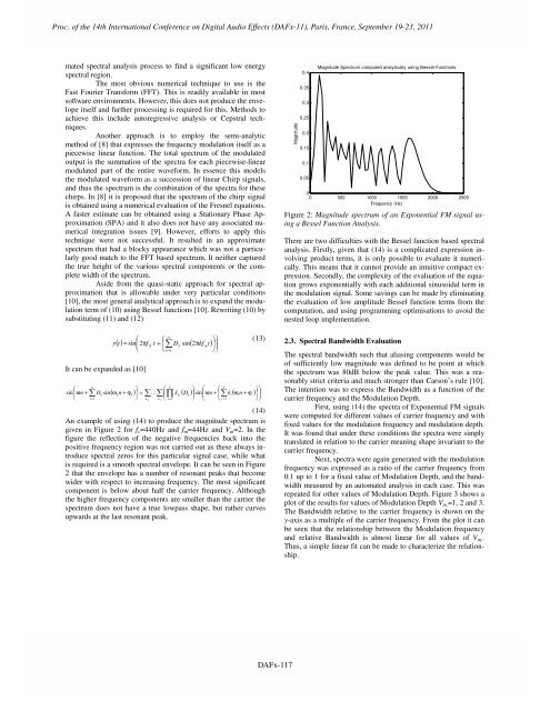
Proc. of the 14th International Conference on Digital Audio Effects (DAFx-11), Paris, France, September 19-23, 2011Proc. of the 14 th Int. Conference on Digital Audio Effects (DAFx-11), Paris, France, September 19-23, 2011mated spectral analysis process to find a significant low energyspectral region.The most obvious numerical technique to use is theFast Fourier Transform (FFT). This is readily available in mostsoftware environments. However, this does not produce the envelopeitself and further processing is required for this. Methods toachieve this include autoregressive analysis or Cepstral techniques.Another approach is to employ the semi-analyticmethod of [8] that expresses the frequency modulation itself as apiecewise linear function. The total spectrum of the modulatedoutput is the summation of the spectra for each piecewise-linearmodulated part of the entire waveform. In essence this modelsthe modulated waveform as a succession of linear Chirp signals,and thus the spectrum is the combination of the spectra for thesechirps. In [8] it is proposed that the spectrum of the chirp signalis obtained using a numerical evaluation of the Fresnel equations.A faster estimate can be obtained using a Stationary Phase Approximation(SPA) and it also does not have any associated numericalintegration issues [9]. However, efforts to apply thistechnique were not successful. It resulted in an approximatespectrum that had a blocky appearance which was not a particularlygood match to the FFT based spectrum. It neither capturedthe true height of the various spectral components or the completewidth of the spectrum.Aside from the quasi-static approach for spectral approximationthat is allowable under very particular conditions[10], the most general analytical approach is to expand the modulationterm of (10) using Bessel functions [10]. Rewriting (10) bysubstituting (11) and (12)It can be expanded as [10]⎛sin⎜ωn+⎝k∑D sin⎛ ⎛=⎜ ∑ ∞ E⎝ ⎝ k=1⎞⎞( t) sin⎜2πft + ⎜ D sin( 2πkft) ⎟ ⎟ y⎞⎛km⎠⎠( ω ) ∑ ∑ ∏ ( ) ⎜kn+ ϕk⎟ = K ⎜ JkDk⎟sinωn+ ⎜∑ki( ωin+ ϕi)iki = 1k k k1 i = 1i = 1⎠⎝k⎞⎠⎛⎜⎝⎛⎝k(13)(14)An example of using (14) to produce the magnitude spectrum isgiven in Figure 2 for f c =440Hz and f m =44Hz and V m =2. In thefigure the reflection of the negative frequencies back into thepositive frequency region was not carried out as these always introducespectral zeros for this particular signal case, while whatis required is a smooth spectral envelope. It can be seen in Figure2 that the envelope has a number of resonant peaks that becomewider with respect to increasing frequency. The most significantcomponent is below about half the carrier frequency. Althoughthe higher frequency components are smaller than the carrier thespectrum does not have a true lowpass shape, but rather curvesupwards at the last resonant peak.⎞⎟ ⎞⎟⎠⎠Magnitude0.40.350.30.250.20.150.10.05Magnitude Spectrum computed analytically using Bessel Functions00 500 1000 1500 2000 2500Frequency (Hz)Figure 2: Magnitude spectrum of an Exponential FM signal usinga Bessel Function Analysis.There are two difficulties with the Bessel function based spectralanalysis. Firstly, given that (14) is a complicated expression involvingproduct terms, it is only possible to evaluate it numerically.This means that it cannot provide an intuitive compact expression.Secondly, the complexity of the evaluation of the equationgrows exponentially with each additional sinusoidal term inthe modulation signal. Some savings can be made by eliminatingthe evaluation of low amplitude Bessel function terms from thecomputation, and using programming optimisations to avoid thenested loop implementation.2.3. Spectral Bandwidth EvaluationThe spectral bandwidth such that aliasing components would beof sufficiently low magnitude was defined to be point at whichthe spectrum was 80dB below the peak value. This was a reasonablystrict criteria and much stronger than Carson’s rule [10].The intention was to express the Bandwidth as a function of thecarrier frequency and the Modulation Depth.First, using (14) the spectra of Exponential FM signalswere computed for different values of carrier frequency and withfixed values for the modulation frequency and modulation depth.It was found that under these conditions the spectra were simplytranslated in relation to the carrier meaning shape invariant to thecarrier frequency.Next, spectra were again generated with the modulationfrequency was expressed as a ratio of the carrier frequency from0.1 up to 1 for a fixed value of Modulation Depth, and the bandwidthmeasured by an automated analysis in each case. This wasrepeated for other values of Modulation Depth. Figure 3 shows aplot of the results for values of Modulation Depth V m, =1, 2 and 3.The Bandwidth relative to the carrier frequency is shown on they-axis as a multiple of the carrier frequency. From the plot it canbe seen that the relationship between the Modulation frequencyand relative Bandwidth is almost linear for all values of V m, .Thus, a simple linear fit can be made to characterize the relationship.DAFX-3DAFx-117