FLOW AROUND A CYLINDER - istiarto

FLOW AROUND A CYLINDER
IN A SCOURED CHANNEL BED
THÈSE NO 2368 (2001)
PRÉSENTÉE AU DÉPARTEMENT DE GÉNIE CIVIL
ÉCOLE POLYTECHNIQUE FÉDÉRALE DE LAUSANNE
POUR L’OBTENTION DU GRADE DE DOCTEUR ÈS SCIENCES TECHNIQUES
PAR
Istiarto ISTIARTO
Insinyur (civil), Gadjah Mada University, Yogyakarta, Indonésie
M.Eng., Asian Institute of Technology, Bangkok, Thaïlande
de nationalité indonésienne
acceptée sur proposition du jury :
Prof. W.H. Graf, Directeur de thèse
Dr. M.S. Altinakar, rapporteur
Dr. M. Cellino, rapporteur
Dr. R. Monti, rapporteur
Prof. Y. Zech, rapporteur
Lausanne, EPFL
2001

– ii –

– iii –
Flow around a Cylinder in a scoured Channel Bed
Abstract
The flow pattern around a cylinder protruding vertically on a scoured channel bed was
experimentally and numerically investigated. Flow in an equilibrium scour hole (the
scouring has ceased) under a clear water regime (no sediment supply into the scour hole)
was considered.
Detailed measurements were obtained with a non-intrusive instrument, the Acoustic
Doppler Velocity Profiler (ADVP), which measures the profiles of the 3D instantaneous
velocity vectors. The measurements were done in different vertical planes positioned
around the cylinder. From the measured data, the spatial distributions of the mean (timeaveraged)
velocities and its turbulence components could be deduced.
The numerical simulations of the flow were performed by using a 3D model, which is
developed based on the approximate solution of the time-averaged equations of motion
and of continuity for incompressible flows by using a finite-volume method. The model
uses the k-� turbulence closure model to compute the turbulence stresses and the Semi-
Implicit Method for Pressure-Linked Equation (SIMPLE) method to link the velocity to
the pressure. The discretisation of the equations were done following the hybrid and
power-law schemes on a structured, collocated, hexahedral, body-fitted grid. While the
essentials of the model are relatively standard, some detailed derivations and
clarifications were elucidated about the boundary conditions and the pressure-velocity
coupling.
The measured velocity data show that a three-dimensional flow establishes itself, which
is characterized by a rotating flow inside the scour hole upstream of the cylinder formed
by a strong downward flow along the cylinder face and a reversed flow along the scour
bed. This structure, which is known as horseshoe vortex, disappears behind the cylinder
where a flow reversal towards the water surface is observed immediately behind the
cylinder. These observations are supported by the numerical simulation.
The measured turbulence intensities show a considerable increase inside the scour hole
and in regions close to the cylinder. The turbulent kinetic energy increases on entering
the scour hole, on approaching the cylinder, and on moving towards downstream regions.
The profiles of the turbulent kinetic energy are characterized by bulges below the original
bed level. Similar observations can be made for the Reynolds stresses.
The numerical simulation under-predicted the turbulent kinetic energy, notably in the
wake region immediately behind the cylinder. It appears that this problem is related to the

– iv –
computation of the turbulent kinetic-energy generation at the solid boundaries. This
problem was identified and discussed.
Estimates on the bed shear-stresses along the plane of symmetry, based on the measured
velocity and Reynolds stress, disclose a diminishing value upon entering the scour hole
and upon approaching the cylinder. Negative values are observed in the upstream scour
bed, which is in accordance with the reversed flow in that region. Moving downstream
and leaving the scour hole, the bed shear-stresses recover towards their value in the
approach flow. Values obtained from the numerical simulation show a similar trend,
having a satisfactory agreement with the ones obtained from the measurements.
The computation of the water surface profile produced results that are in agreement with
the measured one, with the exception for those along the side circumference of the
cylinder. The discrepancy in this region is apparently due to the inaccuracy of the
computation in regions of a strong pressure gradient, such as the case along the cylinder
circumference. Another method of positioning the water surface, employing kinematic
boundary conditions, was proposed and discussed.

– v –
Écoulement à Surface Libre autour d’un Cylindre
dans une Fosse d’Érosion Locale
Résumé
L’écoulement autour d’un cylindre dans une fosse d’érosion a été étudié en effectuant des
mesures dans un modèle réduit et des simulations numériques avec un modèle
hydrodynamique tridimensionnel. Les mesures et les simulations se limitent à un
écoulement avec une profondeur de fosse qui est en équilibre (il n’y a plus d’érosion) et
sans transport solide.
Le travail expérimental s’effectue principalement par des mesures de vitesses
d’écoulement. Un Profileur Vélocimétrique Acoustique Doppler (PVAD) a été utilisé ; ce
dispositif très puissant est capable de mesurer les vecteurs de vitesse instantanés en
plusieurs points de mesures. À partir de ces mesures, les profils des vitesses (moyennées
sur les temps), des intensités de turbulence et des tensions de Reynolds sont obtenus. La
plupart des mesures a été faite sur des plans verticaux autour du cylindre.�
Pour faciliter le travail numérique, un modèle hydrodynamique tridimensionnel a été
développé. Ce modèle est basé sur la représentation en volumes finis des équations de
Reynolds. Il emploie un maillage structuré dont les variables primitives sont définies au
centre des volumes de contrôle. Les flux convectif et diffusif sont calculés par deux
méthodes (hybride et loi de puissance) avec des corrections des termes non orthogonaux.
La méthode SIMPLE (Semi-Implicit Method for Pressure-Linked Equation) établit le
couplage de la pression avec la vitesse ; elle permet le calcul du champ de pression. La
viscosité turbulente est calculée à l’aide du modèle k-�. Le modèle est relativement
standard ; néanmoins, quelques dérivations et clarifications ont été abordées sur les
conditions aux bords et le calcul de pression.
Les données des vitesses mesurées montrent que l’écoulement dans le plan de symétrie
amont s’organise dans un tourbillon créé par l’arrêt de l’écoulement arrivant au cylindre.
La pression due à l’arrêt d’écoulement augmente et, par conséquent, conduit
l’écoulement vers le bas près du cylindre avec une vitesse croissante ; près du fond,
l’écoulement se dirige vers l’amont. Ce tourbillon est le départ de ce qui est appelé le
vortex de fer-à-cheval. Il se propage vers l’aval et son intensité devient faible voire
presque invisible. Derrière le cylindre, un autre courant de retour est observé alors que
celui prés de la surface se dirige vers le cylindre. Ces phénomènes ont été également
vérifiés par les résultats de la simulation numérique.
Les intensités de turbulence s’accroissent vers, en entrant la fosse, en approchant le
cylindre et en allant vers l’aval. Les intensités de turbulence sont caractérisés par des pics

– vi –
qui se trouvent au dessous de la ligne du fond original. La même tendance a été observée
sur les profils des tensions de Reynolds.
L’énergie cinétique turbulente obtenue par la simulation numérique a pu être comparée
avec les mesures. Le modèle a sous-estimé les valeurs mesurées. Il paraît que ce
problème provient de la difficulté du calcul de la génération d’énergie cinétique
turbulente près du bord solide. Ce problème a été identifié et discuté en détail.
Les mesures de vitesse et de tensions de Reynolds près du fond permettent d’estimer la
force de frottement au fond de la fosse ; celle ci a été faite aux plans de symétrie amont et
aval. Elle montre que la force de frottement décroît en entrant dans la fosse et en
s’approchant du cylindre. Des valeurs négatives sont obtenues au plan amont où le
courant de retour est observé. Derrière le cylindre, la force de frottement décroît en
sortant de la fosse. La même tendance a été démontrée par les résultats de la simulation
numérique.
Le profil de la surface d’eau en amont du cylindre concorde avec les mesures. Vers les
plans aval, le résultat de la simulation est moins satisfaisant ; le modèle a sous-estimé la
profondeur de l’eau dans le plan normal de l’écoulement. Ce problème pourrait être dû à
l’imprécision de la méthode de calcul aux endroits ayant un gradient de pression forte.
Une proposition d’amélioration du calcul de la surface libre, en utilisant la condition
cinématique, a été élaborée.

– vii –
Acknowledgements
I wish to express my deepest gratitude and appreciation to my supervisor, Prof.
W.H. Graf, Director of the Laboratoire de Recherches Hydrauliques (LRH) of the École
Polytechnique Fédérale de Lausanne (EPFL), for admitting me to undertake the research
work leading to this dissertation. I consider it as a privilege to work under his
supervision. It is through his inexhaustible guidance, advice, and encouragement that this
work could be accomplished.
I am deeply indebted to Prof. Y. Zech from the Université Catholique de Louvain,
Louvain-la-Neuve, Belgium, with whom I had fruitful discussions during his many stays
at EPFL as a visiting professor and a member of the examination committee. His
constructive ideas and suggestions have certainly contributed a lot to the work,
particularly for the numerical part. I appreciate his careful reading of the manuscript and
the verification he did to all mathematical expressions.
Sincere thanks go to all the members of LRH for their friendships and unconditional
readiness to help. Special appreciation is due to Dr. M.S. Altinakar for the many
rewarding discussions and his willingness to serve as a member of the examination
committee, to Dr. U. Lemmin for providing the experimental facilities, and to
C. Perrinjaquet for his invaluable help in the computer logistic support. Thanks go also to
my fellow (past and present) doctoral students at the LRH: P. Hamm, B. Yulistiyanto,
R. Jiang, C. Shen, M. Cellino, K. Blanckaert, D. Hurther, I. Fer, A. Kurniawan, Z. Qu,
Y. Guan, and I. Schoppe. I thank Dr. M. Cellino for serving as the member of the
examination committee.
I express my thanks to Dr. R. Monti from the Terr@A Hydraulic Research Centre for the
Environment, Departement of IIAR, Politecnico di Milano, Italy, for her constructive
comments while serving as a member of the examination committee. Prof. P. Egger is
acknowledged for his willingness to serve as the chairman of the examination committee.
My special thanks go to Dr. Budi Wignyosukarto and Dr. Djoko Legono from the Civil
Engineering Department, Gadjah Mada University, Indonesia, for their support and
encouragement in my decision to go abroad to undertake this study. Their continuous
help offered to me and to my family is sincerely acknowledged.
Finally, I wish to convey my gratitude to the Swiss Federal Commission on Scholarships
for Foreign Students for providing the financial support during the early phase of the
work.
To all of you, I say a most heartfelt thank you.

– viii –

– ix –
Table of Contents
Abstract iii
Résumé v
Acknowledgements vii
1 Introduction 1.1
1.1 Flow around a cylinder 1.1
1.2 Objective and scope of the work 1.3
References 1.4
2 Flow Measurements 2.1
Abstract 2.1
Résumé 2.2
2.1 Measurement design 2.3
2.2 Experimental setup 2.3
2.2.1 Laboratory channel 2.3
2.2.2 Acoustic Doppler Velocity Profiler (ADVP) 2.5
2.2.3 Other measuring instruments 2.13
2.2.4 Flow parameters 2.14
2.2.5 Experimental procedures 2.14
2.3 Preliminary experiments 2.15
2.3.1 Scour depth measurements 2.15
2.3.2 Time evolution of scour depth 2.16
2.3.3 Comparison to other measurements 2.17
2.3.4 Selected cylinder diameter 2.17
2.4 Velocity measurements in the uniform approach flow (without cylinder) 2.19
2.4.1 Measurement stations 2.19
2.4.2 Vertical distribution of the (time-averaged) velocity 2.20
2.4.3 Vertical distribution of the turbulence intensities 2.22
2.4.4 Vertical distribution of the Reynolds shear-stresses 2.24
2.5 Velocity measurements around the cylinder 2.25
2.5.1 Measurement strategy 2.25
2.5.2 Data presentations 2.27
2.5.3 Measurements in the plane � = 0° 2.28
2.5.4 Measurements in the plane � = 45° 2.35

– x –
2.5.5 Measurements in the plane � = 90° 2.41
2.5.6 Measurements in the plane � = 135° 2.47
2.5.7 Measurements in the plane � = 180° 2.52
2.6 Summary and conclusions 2.57
References 2.58
Notations 2.59
3 Elaboration of the measured Flow 3.1
Abstract 3.1
Résumé 3.1
3.1 Introduction 3.3
3.2 (Time-averaged) velocity fields 3.3
3.2.1 Vertical distribution of the velocity 3.4
3.2.2 Flow pattern around the cylinder 3.7
3.2.3 Transverse velocity 3.11
3.2.4 Vertical velocity (downward flow) 3.15
3.2.5 Vorticity fields 3.20
3.3 Turbulence characteristics around the cylinder 3.22
3.3.1 Vertical distributions of the turbulence stresses 3.22
3.3.2 Turbulent kinetic energy 3.24
3.4 Bed shear-stresses along the plane of symmetry 3.29
3.5 Summary and conclusions 3.34
References 3.38
Notations 3.38
4 Numerical Model Development 4.1
Abstract 4.1
Résumé 4.1
4.1 Governing equations 4.2
4.2 Solution strategy: the iterative method 4.5
4.3 Numerical method: the finite-volume approximation 4.8
4.3.1 Grid arrangement 4.8
4.3.2 Computation of the surface area and of the cell volume 4.9
4.3.3 Cell-face interpolation and gradient computation 4.11
4.3.4 Discretisation of the time derivative terms 4.12
4.3.5 Discretisation of the convective terms 4.13
4.3.6 Discretisation of the diffusive terms 4.14
4.3.7 Convective-diffusive terms: hybrid and power-law schemes 4.16
4.3.8 Source terms 4.19
4.3.9 Assembly of the coefficients 4.22

– xi –
4.4 Pressure-velocity coupling 4.24
4.4.1 SIMPLE algorithm 4.24
4.4.2 Pressure correction procedure 4.28
4.4.3 Under-relaxation factor and time step 4.29
4.5 Boundary conditions 4.29
4.5.1 Boundary placement 4.29
4.5.2 Inflow boundary 4.31
4.5.3 Outflow boundary 4.32
4.5.4 Wall boundary 4.33
4.5.5 Symmetry boundary 4.41
4.5.6 Surface boundary 4.43
4.6 Solution procedures 4.47
4.6.1 Spatial discretisation 4.47
4.6.2 Matrix solvers 4.49
4.7 Summary 4.53
References 4.53
Notations 4.54
5 Numerical Simulation 5.1
Abstract 5.1
Résumé 5.1
5.1 Introduction 5.2
5.2 Experimental data 5.3
5.2.1 Flow around a cylinder on a flat channel bed 5.3
5.2.2 Flow around a cylinder in a scoured channel bed 5.3
5.3 Model calibration of ks and h∞ 5.4
5.3.1 Computational domain 5.4
5.3.2 Boundary and initial conditions 5.5
5.3.3 Calibration results 5.6
5.4 Test run using uniform flow condition 5.8
5.4.1 Boundary and initial conditions 5.8
5.4.2 Results of the test runs 5.9
5.4.3 Conclusions 5.13
5.5 Simulation of flow around a cylinder on a flat channel bed 5.17
5.5.1 Computational domain 5.17
5.5.2 Boundary and initial conditions 5.17
5.5.3 Results of the simulation and comparison to the experimental data 5.19
5.5.4 Conclusions 5.28
5.6 Simulation of flow around a cylinder in a scoured channel bed 5.28
5.6.1 Computational domain 5.28
5.6.2 Boundary and initial conditions 5.29

– xii –
5.6.3 Results of the simulation and comparison to the experimental data 5.31
5.6.4 Conclusions 5.44
5.7 Summary and conclusions 5.44
5.8 Recommendations for future works 5.45
References 5.48
Notations 5.48
6 Summary and Conclusions 6.1
6.1 The work 6.1
6.2 Results 6.1
6.2.1 Laboratory measurements 6.1
6.2.2 Numerical simulations 6.3
6.3 Conclusions 6.4
6.4 Recommendations for future works 6.5
Curriculum Vitae 7.1

Chapter 1
– 1.i –
1 Introduction 1.1
1.1 Flow around a cylinder................................................................................... 1.1
1.2 Objective and scope of the work .................................................................... 1.3
References................................................................................................................... 1.4

– 1.ii –

1 Introduction
1.1 Flow around a cylinder
– 1.1 –
Local scour around a pier is a result of the interaction amongst the pier, the approach
flow and the erodible bed. The presence of a pier results in a stagnation pressure build-up
in front of the pier and a three-dimensional turbulent flow —characterized by the
downward flow ahead of the pier and the so-called horseshoe vortex along the base of the
pier— forms itself. The flow modifies the erodible bed in the vicinity of the pier when
local scour takes place. It has been generally agreed upon that this scour is initiated by
the downward flow and further provoked by the horseshoe vortex. The scour process can
be either a clear-water one when there is no general sediment transport, or a live-bed one
when a sediment transport takes place along the channel. Local scour is a complex
phenomenon due to the interplay among various parameters, namely the fluid, the flow,
the time, the bed material, and the pier. Two particular interests in the study of local
scour around a pier are the development of the equilibrium scour hole as a function of
those parameters and the alteration of the flow field around the pier. This second aspect
has been selected as the object in the present work. The flow field around a cylindrical
pier is studied numerically and experimentally, in which a clear-water flow in an
equilibrium (maximum) scour-depth is considered. This work is a continuation and an
extension of the previous study conducted at the Laboratoire de recherches hydrauliques
(LRH) of EPFL (Yulistiyanto, 1997).
In the work previously conducted at LRH, extensive velocity data of flow around a
cylinder on a flat channel bed were reported (Yulistiyanto, 1997; Graf and Yulistiyanto,
1998). The three-dimensional instantaneous velocities are measured by using an Acoustic
Doppler Velocity Profiler (ADVP) conceived and developed at LRH (Lhermitte and
Lemmin, 1994). The data are presented as the vertical distributions of velocities,
Reynolds stresses, and turbulence intensities in different vertical planes around the
cylinder. It is reported that the horseshoe vortex manifests itself, which depends largely
on the approaching flow; it has the strongest rotation at the plane of symmetry upstream
of the cylinder. Its strength weakens as it travels downstream along the perimeter of the
cylinder. Their measurements show that, as the flow passes the cylinder from upstream
up to the side of the cylinder, the turbulent kinetic energy decreases, but further
downstream the turbulent kinetic energy increases. Upstream of the cylinder, the
maximum energy is concentrated at the bottom corner of the cylinder. This region of
maximum energy at the other planes shifts away from the bed and from the cylinder. In
addition to the laboratory measurements, a numerical simulation of the flow is also
reported (Yulistiyanto, 1997; Yulistiyanto et al., 1998). The depth-averaged velocity field

– 1.2 –
was computed by using a numerical model which takes into account the dispersion
stresses, evaluated from the velocity distributions along the curved streamlines. The
simulation compares favorably with the measurements.
In the light of the previous study results, the work is continued and extended in the
present investigation to embody a scour hole around the cylinder. A similar path is
followed, i.e. by performing numerical flow simulations and by conducting velocity
measurements. The first is aimed at obtaining the general pattern of the velocity alteration
by the cylinder while the second is directed at getting detail pictures of the velocity and
its turbulence structure around the cylinder.
The depth-averaged numerical simulation approach used in the preceding study is not
suitable for the present case since the three-dimensional features of the geometry, i.e. the
scour hole, and the flow are significant. A three-dimensional numerical model is thus
opted. The model is developed based on the approximate solution of the time-averaged
equations of motion and continuity for incompressible flows by using finite-volume
method. The closure model is achieved by using the k-� model (Launder and Spalding,
1974). Non-orthogonal hexahedral cell-centered grid arrangements are used and all
variables are defined in the Cartesian coordinate system. The classical hybrid and powerlaw
schemes (Patankar, 1980) are applied to discretise the convective-diffusive fluxes,
combined with the so-called Semi-Implicit Method for Pressure-Linked Equation
(SIMPLE) method to compute the pressure (Patankar and Spalding, 1972).
The ADVP, as in the preceding study, is used to measure the three-dimensional
instantaneous velocity. The measurements are conducted in the equilibrium (maximum)
scour-depth condition which is established under a clear-water scour regime. Vertical
distributions of the three-dimensional instantaneous velocities are measured at radial
planes around the cylinder, from which the vertical distributions of the (time-averaged)
velocities, the turbulence intensities, and the Reynolds stresses are deduced.
A number of works on local scour around cylindrical piers, both numerical simulations
and experiments, have been reported. Herein a brief summary of those previous works is
presented.
Most of the experimental works on flow around a cylinder so far concern with the
development of the scour depth. Few work have focused on the flow field (see for
example Hjorth, 1975; Melville, 1975; Dargahi, 1987; Dey et al., 1995; Ahmed and
Rajaratnam, 1998; Graf and Yulistiyanto, 1998). Melville (1975) was the first who
conducted velocity measurements around a cylinder in the scour hole. He measured the
flow velocity and its turbulent structure near the bottom and inside the scour hole by
using hot-film anemometer and pitot tube. From the measurements, he was able to
describe the horseshoe vortex as it travels along the perimeter of the cylinder; the strength
of the horseshoe vortex was evaluated. Hjorth (1975) and Dargahi (1987) did a thorough
investigation by measurements, but concern mostly the flat channel-bed case. Dey et al.
(1995) proposed an analytical flow model to analyze the mean flow velocity in the scour
hole based on the velocity data obtained from measurements using a 5-yaw and a 3-yaw

– 1.3 –
pitot tubes. Ahmed and Rajaratnam (1998) attempted to describe the velocity profiles in
the upstream plane of symmetry by using a Clauser-type defect scheme. It was also
reported that, rather than separating from the bed, the approach flow accelerates on
entering the scour hole; a downward velocity up to 95% of the approach velocity was
reported.
Simulations of three-dimensional flow around a cylinder have been reported (see for
example Ali et al., 1997, Olsen and Kjellesvig, 1998). Up to recently, however, there has
not been any comparison of the results to detailed measurements. This is mostly due to
the fact that such data are not always available to modelers. A comparison of the
computed and measured flow, not only the time-averaged velocities but also the
turbulence, would help to define clearly the limitations of a mathematical modeling
approach and, in a broader perspective, to evidence the need for further developments or
refinements of the computational techniques. In this aspect, therefore, the contribution of
the present work shall be considered.
1.2 Objective and scope of the work
The objective of the present work is focused on the obtaining of better understanding to
the flow and turbulence structures around the cylinder as they are altered by the cylinder
and the scour hole. The investigation is limited to the flow in an equilibrium scour-depth
under a clear-water scour regime. The work is implemented through laboratory
experiments by conducting detailed measurements on the three-dimensional velocity and
through numerical modeling by performing three-dimensional flow simulations.
The detailed measurements of the vertical distributions of the three-dimensional
instantaneous velocities are conducted in vertical planes around the cylinder by using
ADVP, a non-intrusive acoustic velocity profiler (see Chapter 2). From those
measurements the distributions of the (time-averaged) velocities, of the vorticities, of the
turbulence intensities, and of the Reynolds stresses can be constructed and investigated
(see Chapter 3). The velocity measurements are performed only for a single run with a
given set of flow parameters and one cylinder diameter. Four observations of scour depth
developments under different flow conditions and cylinder diameters, nevertheless, are
conducted.
The numerical simulations are performed by using a three-dimensional model developed
in the present work (see Chapter 4). The model is based on the approximate solution of
the time-averaged equations of motion and continuity for incompressible flows by using
finite-volume method. The model uses the k-� turbulence closure model to compute the
turbulence stresses and the SIMPLE method to link the velocity to the pressure. The
water surface boundary is determined according to the pressure along the surface
boundary. The model, even though solves the transient flow equations, is applicable only
for steady flow problems. The model is tested to simulate a simple uniform flow to verify
its basic performance. The tested model is then applied to simulate flow around a
cylinder. Two cases of flow around a cylinder are considered, namely flat channel bed

– 1.4 –
and scoured channel bed (see Chapter 5). The simulation results for the flat channel bed
case are compared to the Yulistiyanto’s measurements (Yulistiyanto, 1997). The results of
the scoured channel bed case are compared to the present measurements.�
References
Ahmed, F., and Rajaratnam, N. (1998). ―Flow around bridge piers.‖ ASCE, J. Hydr.
Engrg., 124(3), 288-300.
Ali, K. H. M., Karim, O. A., and O'Connor, B. A. (1997). ―Flow patterns around bridge
piers and offshore structures.‖ Proc. 27th Congress of the IAHR, San Francisco,
California, Theme A, 208-213.
Dargahi, B. (1987). ―Flow Field and Local Scouring around a Cylinder.‖ Bulletin No.
TRITA-VBI-137, Hydraulic Laboratory, The Royal Inst. of Technology,
Stockholm, Sweden.
Dey, S., Bose, S. K., and Sastry, G. L. N. (1995). ―Clear water scour at circular piers: a
model.‖ ASCE, J. Hydr. Engrg., 121(12), 869-876.
Graf, W. H., and Yulistiyanto, B. (1998). ―Experiments on flow around a cylinder; the
velocity and vorticity fields.‖ IAHR, J. Hydr. Res., 36(4), 637-653.
Hjorth, P. (1975). Studies on the Nature of Local Scour., Dept. of Water Res. Engrg.,
Lund Inst. of Technology, Sweden.
Launder, B. E., and Spalding, D. B. (1974). ―The numerical computation of turbulent
flows.‖ Computer Methods in Applied Mechanics and Engineering, 3, 269-289.
Lhermitte, R., and Lemmin, U. (1994). ―Open-channel flow and turbulence measurement
by high-resolution Doppler sonar.‖ J. Atm. Ocean. Tech., 11, 1295-1308.
Melville, B. W. (1975). ―Local scour at bridge sites.‖ Report No. 117, Univ. of Auckland,
School of Engrg., New Zealand.
Olsen, N. R. B., and Kjellesvig, H. M. (1998). ―Three-dimensional numerical flow
modeling for estimation of maximum local scour depth.‖ IAHR, J. of Hydr. Res.,
36(4), 1670-1681.
Patankar, S. V. (1980). Numerical Heat Transfer and Fluid Flow., Hemisphere
Publishing Corp., New York, USA.
Patankar, S. V., and Spalding, D. B. (1972). ―A calculation procedure for heat, mass and
momentum transfer in three-dimensional parabolic flows.‖ Int. J. Heat Mass
Transfer, 15, 1787-1806.
Yulistiyanto, B. (1997). Flow around a cylinder installed in a fixed-bed open channel.,
Doctoral Dissertation, No. 1631, EPFL, Lausanne, Switzerland.
Yulistiyanto, B., Zech, Y., and Graf, W. H. (1998). ―Flow around a cylinder: shallowwater
modeling with diffusion-dispersion.‖ ASCE, J. Hydr. Engrg., 124(4), 419-
429.

Chapter 2
– 2.i –
2 Flow Measurements 2.1
Abstract ...................................................................................................................... 2.1
Résumé........................................................................................................................ 2.2
2.1 Measurement design ....................................................................................... 2.3
2.2 Experimental setup ......................................................................................... 2.3
2.2.1 Laboratory channel ..................................................................................... 2.3
2.2.2 Acoustic Doppler Velocity Profiler (ADVP) ............................................... 2.5
2.2.3 Other measuring instruments ..................................................................... 2.13
2.2.4 Flow parameters ....................................................................................... 2.14
2.2.5 Experimental procedures ........................................................................... 2.14
2.3 Preliminary experiments .............................................................................. 2.15
2.3.1 Scour depth measurements ........................................................................ 2.15
2.3.2 Time evolution of scour depth ................................................................... 2.16
2.3.3 Comparison to other measurements ........................................................... 2.17
2.3.4 Selected cylinder diameter ........................................................................ 2.17
2.4 Velocity measurements in the uniform approach flow (without cylinder) . 2.19
2.4.1 Measurement stations ................................................................................ 2.19
2.4.2 Vertical distribution of the (time-averaged) velocity ................................. 2.20
2.4.3 Vertical distribution of the turbulence intensities ....................................... 2.22
2.4.4 Vertical distribution of the Reynolds shear-stresses ................................... 2.24
2.5 Velocity measurements around the cylinder ............................................... 2.25
2.5.1 Measurement strategy ............................................................................... 2.25
2.5.2 Data presentations ..................................................................................... 2.27
2.5.3 Measurements in the plane � = 0° ............................................................. 2.28
2.5.4 Measurements in the plane � = 45° ........................................................... 2.35
2.5.5 Measurements in the plane � = 90° ........................................................... 2.41
2.5.6 Measurements in the plane � = 135° ......................................................... 2.47
2.5.7 Measurements in the plane � = 180° ......................................................... 2.52
2.6 Summary and conclusions ............................................................................ 2.57
References ................................................................................................................. 2.58
Notations ................................................................................................................... 2.59

– 2.ii –

2 Flow Measurements
Abstract
– 2.1 –
Measured three-dimensional flow fields around a vertical cylinder, in an established
(equilibrium) scour hole under a clear-water regime, are reported. An acoustic Doppler
velocity profiler (ADVP) was used to measure instantaneously the vertical distributions
of the three velocity components in vertical planes around the cylinder. The flow field is
presented as the vertical distributions of the (time averaged) velocities, of the turbulence
intensities, and of the Reynolds stresses in the planes � = 0°, 45°, 90°, 135° and 180°.
The flow in plane of symmetry upstream of the cylinder, � = 0°, is characterized by a
reversed flow along the scour bed and a strong downward flow close to the cylinder. This
structure remains, but with diminishing strength, in the other planes, � = 45°, 90°, and
135°. In these three planes, the downward flow has a decreasing magnitude. In the plane
� = 180°, there is a flow reversal close to the surface. As the flow moves downstream,
leaving the scour hole, the flow reversal diminishes; the flow is recovering to the
approach flow condition. Measurements in all planes show that the flow in the far region,
outside the scour hole, does not change with the presence of the cylinder. The flow is
altered only in the scour-hole region.
The turbulence intensities get stronger in the downstream planes. The increase is notably
important from the plane � = 90° to � = 135° and further downstream to � = 180°.
Approaching the cylinder, in all planes except in the plane � = 180°, the turbulence
intensifies within the scour hole, z < 0, but remains more or less unchanged outside the
scour hole, z > 0. Downstream of the cylinder, in the plane � = 180°, the turbulence gets
its strongest intensities. It is interesting that the three components of the intensity, u �� u ��,
v �� v ��,
and w ��w
��,
in the plane � = 180° indicate a tendency of being isotropic.�
The vertical distributions of the Reynolds stresses in the planes � = 0° to 135° have an
almost linear distribution in the upper layer, z > 0, while in the lower layer, they exhibit a
strong peak. From the plane � = 0° to � = 135°, the Reynolds stresses inside the scour
hole get increasingly stronger. In all planes, the �u �� w �� is always dominant compared to
the �v �� w ��.
Downstream of the cylinder in the plane � = 180°, however, the vertical
distributions of the Reynolds stresses do not show any conclusive trend.
Presented also are the vertical distributions of the uniform approach flow, i.e. the flow
without the cylinder being installed. The approach flow is uniform, but shows a slight
tendency of being decelerated; the bed is hydraulically (incomplete) rough.

Résumé
– 2.2 –
Le champ des vitesse mesuré autour d’un cylindre dans un affouillement est présenté. Un
profileur vélocimétrique acoustique Doppler est utilisé pour effectuer les mesures ; ce
dispositif mesure les trois composantes de vitesse instantanée en plusieurs points de
mesure au long d’un vertical. A partir de ces mesures, les profils des vitesses
(moyennées), des turbulences et des tensions de Reynolds sont obtenues.
Les données des vitesses mesurées montrent que l’écoulement dans le plan de symétrie
amont s’organise dans un tourbillon créé par l’arrêt de l’écoulement arrivant au cylindre.
La pression due à l’arrêt d’écoulement augmente et, par conséquent, conduit
l’écoulement vers le bas près du cylindre avec une vitesse croissante (un maximum de
0.6U ∞ ) ; près du fond, l’écoulement se dirige vers l’amont. Ce tourbillon est le départ de
ce qui est appelé le vortex de fer-à-cheval. Il se propage vers l’aval et son intensité
devient faible voire presque invisible. Derrière le cylindre, un autre courant de retour est
observé alors que celui prés de la surface se dirige vers le cylindre.
Les intensités de turbulence s’accroissent vers les plans aval. Cette augmentation est plus
significative au plan � = 90° au � = 135°, et également au plan � = 180°. Les turbulences
dans la fosse, d’après les mesures sur tous les plans, s’intensifient quand l’écoulement
s’approche du cylindre. Les intensités de turbulence sont au maximum au plan � = 180°.
Il est intéressant de noter que dans ce plan la turbulence ait une tendance à être
isotropique. Les profils de l’énergie cinétique turbulente sont caractérisés par des pics qui
se trouvent à la ligne de séparation.
Les profils des tensions de Reynolds, �u �� w �� et �v �� w ��,
sont à peu près linéaires dans la
partie supérieure, z > 0, alors que dans la fosse, z < 0, ils montrent une forte croissante
vers le maximum. Du plan � = 0° aux plans � = 45°, 90° et 135°, les tensions de
Reynolds dans la fosse augmentent. Dans tous les plans, la composante �u �� w �� est
toujours supérieure par rapport au �v �� w ��.
Derrière le cylindre, la répartition des tensions
de Reynolds ne donne pas de tendance concluante.
Des mesures ont été aussi effectuées dans l’écoulement à fond plat sans cylindre ; cellesci
représentent les conditions d’approche. Les profils mesurés indiquent que l’écoulement
d’approche est uniforme et a une tendance à décélérer et hydrauliquement en transitionrugueux.�

2.1 Measurement design
– 2.3 –
The flow measurement is aimed at collecting detailed data of the three-dimensional
velocity fields around the cylinder, from which a close investigation can be made to
characterize the alteration of the flow around the cylinder. A series of measurements shall
be performed around the cylinder in an equilibrium scour-depth under a clear-water scour
regime. An equilibrium scour-depth is defined as the depth of scour hole in front of the
cylinder that has no longer changed appreciably under a continuous (steady) flow. A
clear-water scour regime prevails when the scouring process is due solely to the
interaction of the flow with the obstruction (the cylinder) and that the sediment transport
does not exist in the approach flow. A live-bed scour prevails otherwise.
The ADVP shall be used to obtain the vertical distributions of the instantaneous threedimensional
velocities. The measurements are to be performed at stations distributed
along vertical planes around the cylinder, outside and inside the scour hole. The hydraulic
parameters of the experiment are selected according to certain criteria relating to the
scouring mechanism and the available laboratory facilities and instrumentation. In terms
of the scouring process, the flow has to maintain a clear-water scour and result in a
maximum scour depth for the given sediment and cylinder diameter. This can be
achieved with flows having a velocity close to but less than the sediment entrainment
velocity. From the instrument point of view, the scour-hole depth shall be small to keep
the entire flow depth in the range of the instrument measuring capability.
Given in the following sections are the detailed aspects of the measurements, from the
setup to the results of the measurements.
2.2 Experimental setup
2.2.1 Laboratory channel
The experiments were conducted in a 29 [m] long and 2.45 [m] wide rectangular
erodible-bed channel. This wide channel allows for flows with sufficiently large aspect
ratio in terms of the flow depth and cylinder diameter. Large ratios of channel width, B,
to cylinder diameter, Dp, guarantee that the flow around the cylinder is a manifestation of
the interaction between the approaching flow and the cylinder. In the present work, this
ratio is B D p = 16, being sufficiently higher than the generally agreed minimum ratio of
B D p > 8. The large ratios of the channel width to the flow depth, h ∞ , ensure the
approaching flow to be a quasi two-dimensional one where the side wall does not
influence the flow. In the present work, the ratio is B h = 13.6; this is higher than the
minimum value usually taken as the criterion, B h > 7. The general view of the channel
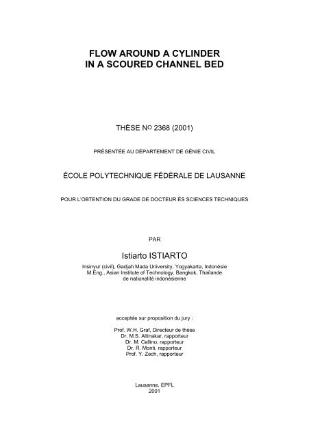
is shown in Fig. 2.1 and its principal elements are presented in the following paragraphs.

– 2.4 –
Fig. 2.1 General view of the channel.

– 2.5 –
The water circuit is a closed loop in which clear water is circulated. The flow is
generated from the general sump (1) by a 0.250[m 3 /s]-capacity pump (2), flowing
through the hydraulic circuit (3), passing the operating valve (4) and the electro-magnetic
flow-meter (5), entering the channel through the perforated pipe (6) and the channel inletbasin
(7). After the inlet basin, a type of honeycomb (8) is provided to distribute evenly
the flow over the upstream section of the channel. At the downstream of the honeycomb,
a floating plate (9) is installed to stabilize the water surface. The water flows along the
channel, passes through the working reach (10) at 10.5 [m] ≤ x L ≤ 14.25 [m] (x L is the
distance from the entrance) where the cylinder (11) is vertically installed at x L = 11 [m].
A basin (12) is provided at the downstream reach to trap the transported sediment. Before
leaving the channel and going back to the general sump, the water passes through a
motor-regulated tailgate (13), which is used to control the water-depth in the channel.
The mobile-bed is made of a uniform sand (14) having a mean diameter of d 50 = 2.1 [mm]
and a distribution ratio of � g = 1.3. The sand layer is 50 [cm] in the working reach and
10 [cm] along the rest of the channel. The sand layer is separated from the bottom of the
channel by a geotextile-sheet (15) and a layer of gravel (16). These layers avoid the
deformation of the sand layer when the channel is being slowly filled (at the beginning of
the experiment) or drained (at the end of the experiment) through the bottom pipes (17).
The measuring instrument, ADVP, is mounted on a measuring carriage (18) having a
three-axis positioning equipment allowing the instrument to be positioned at any point
along and across the channel.
2.2.2 Acoustic Doppler Velocity Profiler (ADVP)
Working principles
The Acoustic Doppler Velocity Profiler (ADVP) conceived and developed at LRH
(Lhermitte and Lemmin, 1994) is the main measuring instrument in the present work.
This non-intrusive instrument measures the instantaneous velocity vector at a number of
layers within the water column. The ADVP has been extensively exploited in the research
works conducted at LRH. Its modular installation allows a high flexibility in its use.
Several different configurations have been used in different measurements conducted
previously at LRH. This section describes the one used in the present work; given also
are the procedures of the measurement and of the velocity abstraction. Detail technical
descriptions of the instrument can be found in reports and publications elsewhere
(Lhermitte and Lemmin, 1994; Rolland, 1994; Hurther et al., 1996).
The ADVP measures the velocities in a water column based on the back-scattered
acoustic wave information. An emitting transducer sends an acoustic wave across the
water column. Upon hitting a target moving with the flow, the wave is reflected and
captured by one or several receiving transducers. The target can be air bubbles,
suspended particles, or density fronts due to temperature differences. Knowing the
frequency difference between the emitted and reflected ones, the so-called Doppler

– 2.6 –
frequency, the velocity of the moving target can be deduced. To obtain profiles of the
velocity across the water depth, the recording time of the reflected waves is gated
according to a predetermined interval. This time gate determines the height of the
measured target. The diameter of the target is obviously determined by the diameter of
the acoustic beam from the emitting transducer.
Instantaneous velocity
The derivation of the instantaneous velocity from the measured Doppler frequency
depends, among others, on the configuration and/or the placement of the emitter and
receivers. Several configurations have been used in the measurement works at LRH; they
are largely determined by the geometry of the measurement fields. For the present work,
� � – �
, T1 , T2 , T2 ,
the set-up consists of one conical emitter, T 3 , and four plane receivers, T 1
which are arranged according to Fig. 2.2.
Fig. 2.2 Configuration of the ADVP instrument used in the velocity measurement:
(a) top view, (b) side view along section I-I, (c) velocity derivation along the tristatic
� �
plane T3T1 , and (d) velocity derivation along the tristatic plane T1 T3.

– 2.7 –
Consider a target ―i‖ moving with the flow, passing the acoustic beam emitted from the
� �
ADVP as shown in Fig. 2.2a,b where the vertical plane T1 T3T1 is shown (the vertical
� �
plane T2 T3T2 is analogous). The dimension of the target constitutes the measuring
volume which depends on the diameter of the acoustic beam (determined by the type of
the emitter T3), its distance from the emitter, and the recording time-gate interval. This
will be described in the later section.
The three-dimensional instantaneous velocity, ˆ V �u ˆ , ˆ v , w ˆ �, is measured by the ADVP as a
pair of two-dimensional instantaneous velocities, ˆ V 1�u ˆ 1, w ˆ 1�
and ˆ V 2�u ˆ 2, w ˆ 2�,
i.e. the
� � � �
projections of the target velocity on the vertical planes T1 T3T1 and T2 T3T2 ,
respectively. Both velocities are identified by their components along the longitudinal
direction, u ˆ 1 or u ˆ 2 , and along the vertical direction, w ˆ 1 or w ˆ 2 , of the respective planes.
� � � �
The system of one emitter and a pair of receivers T1 T3T1 or T2 T3T2 is called a tristatic
mode measurement and the vertical plane formed by the system is called a tristatic plane.
By geometrical relationships, the two measured velocity components, ˆ V 1 u ˆ 1, ˆ
� � and
V ˆ
2�u ˆ 2, w ˆ 2�,
can be combined to give the target velocity, ˆ V �u ˆ , ˆ v , w ˆ �. The following
paragraphs describe the derivation of the target’s velocity; the procedure follows the one
given by Rolland (1994). Details are given for the derivation of the velocity component
V ˆ
1 u ˆ 1, ˆ
� � by referring to Fig. 2.2c,d; an analogy applies to the other component.
w 1
� �
The instantaneous velocity component along the tristatic plane T1 T3T1 , V ˆ
1 u ˆ 1, w ˆ 1
� �
(Fig. 2.2c) and T1 T3 (Fig.
w 1
� �, is
obtained from the Doppler frequency measurement by T3T1 �
2.2d) transducers. The frequency difference recorded by the T3T1 transducers can be
related to the target velocity ―seen‖ by this couple of transducers according to the
following expression (Rolland, 1994):
� fe fD �
c
�� s
��
��
ˆ
��
�
V 1
� �� �
e 1 � V ˆ �� ��
3 � e 3��
��
(2.1)
� �
where fD is the Doppler frequency recorded by the T3T1 , fe is the emitted frequency, cs is
�� � ��
the speed of acoustic wave in water, and
��
e 1 and e 3 are the unit directional vectors of
�
T1 and T3 , respectively. From the geometrical relationships (see Fig. 2.2c), one can
write:
�
V ˆ 1
� �� �
e 1 � V ˆ
1
� � ˆ
ˆ
��
V 3 � ��
e 3 � ˆ �
V 3 � ˆ
�
u 1 sin �D,1
�
w 1
� � �
� ˆ cos�D,1
w 1
(2.2)
i� i�
in which u ˆ 1 and w ˆ 1 are the longitudinal and vertical components, respectively, along
�
transducers. Inserting the above
� �
the tristatic plane T1 T3T1 as measured by the T3T1 relation into Eq. 2.1 yields:

� fe fD,1 �
cs – 2.8 –
� � � �
�u ˆ 1 sin� D,1 � w ˆ 1�1�
cos�D,1 ��
(2.3)
By analogy, similar relations as Eqs. 2.1 to 2.3 exist for the Doppler frequency recorded
� �
by the transducer T1 T3 (see Fig. 2.2d). The analogy of Eq. 2.1 for the transducers T1 T3
reads:
� fe fD �
c
�� s
��
��
ˆ
��
�
V 1
� �� �
e 1 � V ˆ �� ��
3 � e 3��
��
and by using geometrical relationships (see Fig. 2.2d), it can be shown that:
�
V ˆ 1
� �� �
e 1 � V ˆ
1
� � ˆ
ˆ
��
V 3 � ��
e 3 � ˆ �
V 3 � ˆ
�
u 1 sin �D,1
�
w 1
� � �
� ˆ cos�D,1
w 1
Thus, one can rewrite Eq. 2.4 as:
� fe fD,1 �
cs (2.4)
(2.5)
� � � �
�u ˆ 1 sin� D,1 � w ˆ 1�1�
cos�D,1 ��
(2.6)
� �
If the systems of T1 T3 and T3T1 are symmetrical about the T3-axis and the measuring
volume of the two systems is the same, one may write:
� � � � � �
�D,1 � �D,1 � �D,1 , ˆ � ˆ � u ˆ 1 , and ˆ � ˆ � ˆ
u 1
u 1
w 1
Therefore, the instantaneous velocity component u ˆ 1 and w ˆ 1 can be extracted from Eqs.
�
system as follows:
�
2.3 and 2.6, obtained from the T1 T3T1 � � � � fD,1�
u ˆ 1 � cs fD,1 2 fe sin�D,1 w 1
� � � � fD,1�
and w ˆ 1 � cs fD,1 2 fe 1� cos� D,1
w 1
� � (2.7)
The above relations give the two-dimensional velocity component, ˆ V 1�u ˆ 1, ˆ �, of the
three-dimensional velocity of the target, ˆ
i
V ˆ
�
on the tristatic plane formed by the T1 T3T1 w 1
i
�u , v ˆ , w ˆ �; this is the projection of ˆ V �u ˆ , v ˆ , w ˆ �
�
transducers. The other two-dimensional
velocity component, ˆ V 2�u ˆ 2, w ˆ 2�,
can be worked out by analogy to Eq. 2.7 for the tristatic
�
. This yields the following expressions:
�
plane T2 T3T2 � � � � fD,2�
u ˆ 2 � cs fD,2 2 fe sin�D,2 � � � � fD,2�
and w ˆ 2 � cs fD,2 2 fe 1� cos� D,2
� � (2.8)

– 2.9 –
Obtaining the velocity components along the two planes, ˆ V 1 u ˆ 1, ˆ
� � and ˆ
w 1
V 2�u ˆ 2, ˆ �, it is
possible to deduce the three-dimensional instantaneous velocity, ˆ V �u ˆ , v ˆ , w ˆ �. In order to
do this, however, it is necessary that the two velocity components be measured from the
� � �
, T2 , T2 ,
same measuring volume. This can only be guaranteed if the four receivers, T1 �
and T2 are placed at the same radial distance with respect to the emitter T3 and at the
same plane (co-planar) that is parallel to the reference plane (see Fig. 2.2c). If, in
addition, the emitter T3 is vertical, one may write for the vertical velocity component:
w ˆ 1 � w ˆ 2 � w ˆ
(2.9)
To obtain the horizontal velocity components, (the u ˆ - and v ˆ -components), the measured
velocities along the two tristatic planes, ˆ V 1�u ˆ 1, ˆ � and ˆ V 2�u ˆ 2, ˆ �, are first projected on
the horizontal plane to give a resultant horizontal velocity, ˆ V h�u ˆ , v ˆ �, whose direction is
� �
T1 (see Fig. 2.3). Using geometrical relationships, one writes:
�V with respect to the T 1
� for the triangle ACA �� : AC �
� for the triangle OAC: V ˆ
h � ˆ
A �� A
w 1
sin� T
�u 1�
2 � AC 2
1 2
� �
� ˆ u 2 � u ˆ 1 cos� T
sin�T � � � �
where �T is the angle of the tristatic-plane T2 T2 with respect to T1 T1 .
Fig. 2.3 Derivation of the instantaneous horizontal velocity component, ˆ V h�u ˆ , v ˆ �,
along the tristatic planes: (a) for u ˆ 1 � 0 , and (b) for u ˆ 1 � 0 .
The horizontal velocity component is thus:
w 2
i
w 2

��
V ˆ
h � �� ˆ
��
��
� � 2 � ˆ ��
u 1
��
��
u 2
2
1 2
� ˆ u 1 cos� �� ��
T
�� ��
sin� T ��
��
��
– 2.10 –
The velocity direction, �V, is given by the relations below:
�V � arcsin ˆ ��u
2 � u ˆ 2 cos� ��
T
��
V ˆ ��, if u ˆ 1 � 0
�� h sin� T ��
�V � 180
��
� � arcsin ˆ ��u
2 � u ˆ 2 cos� �� T
��
��
V ˆ
h sin� T ��
�� , if u ˆ 2 � 0
(2.10)
(2.11)
The three relations, Eqs. 2.9, 2.10, and 2.11, are the ones required to describe the threedimensional
instantaneous velocity of the moving target. It is, however, more convenient
to describe the velocity by its components along the Cartesian or cylindrical coordinate
system. The following section discusses the decomposition of the velocity into those
components.
Cartesian and cylindrical velocity components
The Cartesian coordinate axes are defined as x, y, and z for the horizontal, transversal,
and vertical directions, respectively. The cylindrical coordinate axes are defined as r,
���� = � – 180°), and z for the radial, angular, and vertical directions, respectively (see
Fig. 2.4). The origin of the two coordinate systems is defined at the center of the cylinder,
at the original (uneroded) bed level.
The decomposition of the velocity into its components along the Cartesian and cylindrical
coordinate systems depends on the orientation of the ADVP with respect to the
coordinate system. In the measurements, the instrument is positioned along radial planes
around the cylinder. Fig. 2.4 shows a typical placement of the ADVP and the
decomposition of the velocity into its components along the Cartesian and cylindrical
coordinate systems.
By using geometrical relationships, the Cartesian velocity components can be obtained
from the following expressions:
� �
� �
u ˆ � ˆ V h cos � � �R � � V
v ˆ � ˆ V h sin � � �R � � V
w ˆ � w ˆ 1 � w ˆ 2
where the definitions of the angles are given in Fig. 2.4.
(2.12)

– 2.11 –
Fig. 2.4 Cartesian and cylindrical coordinate systems and the decomposition of the
measured instantaneous velocity into its components in these coordinate systems.
The velocity components along the Cartesian and the cylindrical coordinate systems are
interchangeable by using transformation functional expression as follows:
��u
ˆ r ��
�� ��
�� u ˆ � ��
��
��w
ˆ
��
��
�
��cos�
sin � 0��
��u
ˆ ��
��
��
�sin� cos� 0
�� �� ��
�� ��v
ˆ ��
�� �� 0 0 1��
�� ��
�� w ˆ
��
��
�
�� �cos� �sin � 0��
��u
ˆ ��
��
��
sin� �cos� 0
�� �� ��
�� ��v
ˆ ��
�� �� 0 0 1��
�� ��
��w
ˆ
��
��
��u
ˆ ��
�� ��
��v
ˆ ��
��
�� w ˆ
��
��
�
�� cos� �sin� 0��
��u
ˆ r ��
��
��
sin � cos� 0
�� �� ��
�� ��u
ˆ � ��
�� �� 0 0 1��
�� ��
��w
ˆ
��
��
�
���cos�
sin � 0��
��u
ˆ r ��
��
��
�sin� �cos� 0
�� �� ��
�� ��ˆ
u � ��
�� �� 0 0 1��
�� ��
��w
ˆ
��
��
(2.13a)
(2.13b)
where ˆ
u r, ˆ
u � , and ˆ
w are the radial, angular, and vertical velocity components,
respectively, along the cylindrical coordinate system, (r,�,z), whose origin is defined at
the center of the cylinder.
Time-averaged and fluctuating velocity components
Obtaining the instantaneous velocity data over the measurement period, the statistical
parameters can be found. Three quantities are computed, i.e. the mean (the time-averaged
velocities), the variance (the squared values of the turbulent intensities), and the
covariance (the Reynolds stresses).

– 2.12 –
The time-averaged velocity components are obtained by:
u � u ˆ � 1
N V
v � v ˆ � 1
NV w � w ˆ � 1
NV N V
� (ˆ u ) j,
j�1
N V
� (ˆ v ) j,
j�1
N V
�
j�1
( w ˆ ) j
(2.14)
where NV is the number of instantaneous velocities obtained from the measurement.
Having the time-averaged velocity, the fluctuating components, defined as the deviation
of the instantaneous velocity with respect to the time-averaged value, can be computed
by:
u ���
u ˆ � u, v ���
ˆ v � v, and w ���
w ˆ � w (2.15)
The turbulence (the Reynolds) stresses can thus be obtained by:
u ��u
���
v ��v
���
w ��w
���
1
NV �1
1
NV �1
�u �� w ���
�
�v �� w ���
�
N V
�
j�1
N V
�
j�1
N V
2 �(ˆ u � u) j ��
u ˆ
2 �(ˆ v � v) j ��
v ˆ
� �
1
2 � ( w ˆ � w) j � w ˆ
N V �1
j�1
1
N V �1
1
N V �1
N V
�
j�1
N V
�
j�1
� � 2 � u 2 (2.16a)
� � 2 � v 2 (2.16b)
� � 2 � w 2 (2.16c)
�(ˆ u � u) j( w ˆ � w) j��
��u ˆ w ˆ �� uw (2.16d)
�(ˆ v � v) j( w ˆ � w) j��
��v ˆ w ˆ �� vw (2.16e)
Measuring volume, frequency, and duration of velocity acquisition
The derivation of the Doppler frequency by the ADVP is implemented by recording the
emitted and reflected wave frequencies. The emitting transducer, T3, sends a series of
short trains sinusoidal acoustic waves (pulse) repetitively at a regular time interval (the
pulse repetition frequency, PRF). Between two successive pulses, the receiving
� � � �
transducers, T1 , T1 , T2 , and T2 receive the back-scattered signals. The electronic
system of the ADVP detects and records the intensity and the phase of the incoming
signals at every receiver. The recording process is gated in time in which one time-gate,
Tg, corresponds to one target. The instantaneous velocity is deduced from the velocity of
the target, the volume of which, therefore, represents the measuring volume. The
diameter of the target is determined by that of the acoustic beam emitted from the
transducer T3, where as its thickness is defined by the time-gate, Tg. Two types of

– 2.13 –
transducer were used, a focused-type and a plane-type transducers. The focused-type
transducer was used for measurements at depth h ≤ 18 [cm] where the time-gate was
specified to Tg = 4 [�s]. The measuring volume has a dimension of (see Fig. 2.2b):
thickness �d � 3 [mm], diameter �� � 6 [mm]. The plane-type transducer was used for
measurements at depth h > 18 [cm] with the time-gate fixed at Tg = 6 [�s]. In these
measurements the measuring volume has a dimension of: thickness �d � 4.5 [mm],
diameter 9 � ��[mm] � 26 .
To obtain the time series of the instantaneous velocities of a target, the recorded
intensities and phases of the signals are grouped in which each group contains a number
of intensity-phase data-pairs obtained from several pulses (the number of pulse-pairs,
NPP). A value of NPP of 32 is used in the present work. From each group, one Doppler
frequency is obtained at each receiver. The instantaneous velocity can then be derived
from the Doppler frequency according to Eqs. 2.7 and 2.8. There exists, therefore, a
relation between the pulse frequency, PRF, the number of pulse-pairs, NPP, and the
frequency of the data acquisition, fV:
f V � PRF NPP (2.17)
If the acquisition is done within the duration of Tacq, the number of instantaneous
velocities, NV, for one measurement is:
N V � f V � T acq
(2.18)
The measurements in the present work were conducted with a data acquisition frequency
of fV = 20.8 to 28.4 [Hz] (PRF = 667 to 909 [Hz]). The duration of the acquisition was
Tacq = 150 [s] for measurements at the uniform approach flow and was Tacq = 60 [s] for
measurements around the cylinder. There are thus 3,140 instantaneous velocity data at
every gate (measurement point) for the measurements at the uniform approach flow,
while for the measurements around the cylinder there are 1,250 to 1,700 data.
2.2.3 Other measuring instruments
Besides the ADVP, some other measuring equipment were employed for different
purposes:
� Point-gauge limnimeter: to map the water surface and the channel bed.
� Periscope: to measure the scour depth. The equipment is inserted in the cylinder,
which is transparent. The scour bed can be easily viewed through the mirror provided
at the periscope.
� Electro-magnetic discharge meter: to detect the discharge passing through the circuit.
� Theodolite: to measure the slope of the channel bed.

B
[m]
2.2.4 Flow parameters
– 2.14 –
The experiment is designed such that the scour hole is at its maximum depth for a given
diameter of the cylinder, but a clear-water scour is still maintained. This can be achieved
if the flow velocity is lower than but close to the sediment entrainment velocity. Given
the available sediment size of d50 = 2.1 [mm] and a predetermined bed slope of
So = 0.00055, a preliminary run without the cylinder was performed. The discharge and
the flow depth were regulated such that the sediment particles were about to move and a
uniform flow depth was maintained along the working reach. It was found that the
discharge is of Q = 0.2 [m 3 /s], the flow depth is of h � � 0.18 [m] and the average
velocity is of U � � 0.45 [m s].
The diameter of the cylinder is dictated by the measurement’s technical factors. The
present configuration of the ADVP cannot measure the zone closer than 3 [cm] from the
leading edge of the cylinder and the zone deeper than 50 [cm] from the water surface.
The first constraint suggests that big cylinders are preferred to small ones since the
closest measured profile will be very close with respect to the diameter of the cylinder.
The second constraint, on the other hand, limits the diameter of the cylinder since the
bigger the cylinder, the deeper the scour will be. From those criteria, and after conducting
some preliminary test runs, the diameter of the cylinder was determined as Dp = 15 [cm].
Table 2.1 summarizes the pertinent hydraulic parameters of the present measurement.
So
[10 –4 ]
Q
[m 3 /s]
h∞
[cm]
Table 2.1 Hydraulic parameters of the experiment
B/h∞
[cm]
U∞
[m/s]
Fr
[–]
Re h
[–]
d 50
[mm]
D P
[cm]
Re Dp
[–]
B D P
[–]
h � D p
2.45 5.5 0.2 18 13.6 0.45 0.34 81,000 2.1 15 67,500 16.3 1.2 70
2.2.5 Experimental procedures
The experimental procedures basically consist of three major steps.
(1) Measurements of velocity of the uniform (approaching) flow. Without the cylinder,
a uniform flow was established in the channel; measurement of the corresponding
velocity was then carried out. This step is aimed at obtaining velocity data of the
flow ―unperturbed‖ by the cylinder. The data serve as the reference data with which
the measured data around the cylinder shall be compared.
(2) Establishment of the scour hole. The cylinder was vertically mounted in the
working reach of the channel, at 11 [m] from the entrance. Starting with a flat bed,
the flow was released and allowed to erode the sediment around the cylinder. The
time development of the scour depth at the leading edge of the cylinder was
monitored. The flow was maintained until the equilibrium scour depth was
obtained, that is when it has no longer appreciably changed. A 5-to-7 day run was
[–]
D P d 50
[–]

– 2.15 –
typically needed for this purpose. The channel was drained and the scour geometry,
considered as the (near) equilibrium one, was mapped by point-gauge measurement.
(3) Measurements of the flow fields around the cylinder. Vertical distributions of the
velocity vector were measured at radial planes of �� � � n �15 � , n = 0, 1, 2, ..., 12. A
number of 15 to 25 profiles were obtained at each plane. Due to technical reasons,
the flow had to be occasionally stopped between measurements. In such a case, care
was taken in restarting the flow such that the scour geometry was not disturbed.
When a run was stopped, the water in the channel was slowly evacuated through the
bottom pipes. To restart the run, the water was carefully supplied into the channel
from the same pipes until a sufficient water depth was obtained in the channel. The
supply was then replaced by pump through the hydraulic circuit. The discharge was
regulated, starting with a small one and being gradually increased until the designed
one. The flow depth at the channel was, at the same time, adjusted by regulating the
tailgate.
2.3 Preliminary experiments
2.3.1 Scour depth measurements
Before arriving to the flow parameters selected for the velocity measurements (see Table
2.1 in Sect. 2.2.4) a series of preliminary experiments had been carried out. These
experiment tests provided also knowledge of the scour processes, notably the time
development of the scour depth. Four preliminary runs were performed, namely Test 1, 2,
3 and 4, with the cylinder diameters of D p = 11, 10, 15, and 20 [cm]. The hydraulic
parameters of these test runs are listed in Table 2.2. During the test runs, some
modifications were made to the experimental installation to get the best hydraulic
performance, such as improvements made to the inlet and the outlet sections.
Test
Table 2.2 Hydraulic parameters of the preliminary experiment
d 50
[mm]
Q
[m 3 /s]
h ∞
[m]
D p
[m]
d s
[m]
D p /d 50
[–]
h ∞ /D p
[–]
d s /D p
[–]
1 2.1 0.220 0.170 0.11 0.174 52.38 1.54 1.55
2 2.1 0.250 0.232 0.10 0.195 47.62 2.32 1.95
3 2.1 0.250 0.232 0.15 0.259 71.43 1.55 1.73
4 2.1 0.250 0.232 0.20 0.319 95.24 1.16 1.60
In the test runs only the time development of the scour depth was measured; the velocity
was not measured. Visual observation, however, suggested that the bed particles were
about to move, thus U U cr � 1, where U cr is the critical velocity for particle entrainment.
The scour depth measurements were made at the leading edge of the cylinder where the

– 2.16 –
maximum depth was observed. The cylinder was transparent allowing the measurements
be made from inside the cylinder with the help of a periscope. The equilibrium scour
depths obtained after about 120 [hours] for all tests are shown in Table 2.2.
2.3.2 Time evolution of scour depth
The time histories of the scour depth are depicted in Fig. 2.5a,b plotted in normal and
logarithmic scales.
Observation of the scour development within the first 3 to 5 [minutes] revealed that the
scouring process was very active. The scour initiated at two points approximately 90° to
the right and left off the centerline. The initial scouring propagated upstream along the
perimeter of the cylinder and the two scours met at the leading edge of the cylinder. The
scour depth increased rapidly that at the end of the first hour it reached 50% of the
equilibrium depth. The rate of scour slowed down during the next 48 [hours], after which
the scour depth did not show a significant increase. In the fifth day the scour depth did
not change appreciably; the scour geometry thus obtained was considered as a near
equilibrium one.
The equilibrium scour depths from the four test runs are in the range of
1.55 � d s D p � 1.95, which are in the range of the measurements reported in the literature
(see Fig. 2.6 and the discussion given in the next section).
Fig. 2.5 Relative scour depth at clear water scour versus time in (a) the normal scale and
(b) the logarithmic scale

– 2.17 –
2.3.3 Comparison to other measurements
Various factors affect the scour depth; those are the fluid, the flow, the sediment, and the
cylinder itself (Breusers et al., 1977; Breusers and Raudkivi, 1991; Graf and Altinakar,
1996). The time may also have an effect (Melville, 1975). A general function relating the
relative scour depth, ds/Dp, to the dimensionless parameters is given as follows (Graf and
Altinakar, 1996):
d s
D p
� f U ��
��
��
U cr
, h
,
Dp d
Dp ��
; �g, �s, ���� ��
(2.19)
in which d is the sediment diameter, �g, �s and �� are dimensionless correction
coefficients due to the sediment grading, pier shape, and pier alignment, respectively. The
influence of those coefficients on the relative scour depth is given in graphical forms
based on various measurement data (see Graf and Altinakar, 1996); it is reproduced here
in Fig. 2.6. For a cylindrical pier aligned with the flow as in the present experiment, there
is not any correction due to neither the shape nor alignment of the pier, �s = �� =1.
Putting the results of the present measurements on these graphs, it can be seen that the
effect of the flow velocity and flow depth agrees reasonably with the other measurements
(see Fig. 2.6a,b). The effect of the sediment diameter in the present measurements,
however, underestimates the scour depth when compared with the other measurements
(see Fig. 2.6c). The coefficient of sediment grading, �g, —taking as �g = 0.9 (see Fig.
2.6d)— may explain partially this underestimation.
2.3.4 Selected cylinder diameter
Based on those preliminary experiments and technical considerations relating to the
ADVP configuration, the D p = 15 [cm] cylinder was selected for the experiment with the
velocity measurements (see Sect. 2.2.4). The flow parameters were modified slightly, by
selecting a smaller discharge, Q = 0.200 [m 3 /s], and accordingly a lower flow depth,
h∞ = 18 [cm] (see Table 2.1). The maximum scour depth with this selected flow
parameters is ds = 25 [cm] (ds/Dp = 1.7), which was obtained after a 5-day of continuous
run. Fig. 2.7 shows the geometry of this scour hole. The ridge formed by the deposition
of the bed material in the downstream section extends up to 5 [m] from the cylinder; the
original bed level was found 0.5 [m] further downstream.

– 2.18 –
Fig. 2.6 Comparison of the measured relative scour depth with other measurements
(see Graf and Altinakar, 1996)

– 2.19 –
Fig. 2.7 Scour hole geometry obtained with the selected flow configuration,
Q = 0.200 [m 3 /s], U∞ = 0.45 [m/s], h∞ = 18 [cm], and Dp = 15 [cm].
2.4 Velocity measurements in the uniform approach flow (without
cylinder)
2.4.1 Measurement stations
The measurement of velocity in the uniform flow (it will be the approach flow when the
cylinder is installed) is intended to provide the reference flow data, which shall be useful
later in analyzing the flow data from the measurements around the cylinder.
Six vertical distributions of velocity were measured at stations xL [m] = 9, 10, 11, 12, 13,
and 14 along the centerline of the channel. At each station, 52 data points are obtained

– 2.20 –
throughout the flow depth. The velocity was measured at a frequency of 20.8 [Hz] during
150 [s]; this produces a total number of instantaneous velocities of 3140 at each data
point. The measurement data are presented in the form of vertical distributions of the
time-averaged velocity, of the turbulence intensity, and of the Reynolds stress. The
Cartesian coordinate system is used.
2.4.2 Vertical distribution of the (time-averaged) velocity
Fig. 2.8 shows the vertical distributions of the time-averaged velocities measured at the
six stations. For writing simplicity the term ―velocity‖, otherwise explicitly stated, will be
used to describe the time-averaged velocity. In uniform flows, the vertical distribution of
the longitudinal velocity, u(z), can be described by the universal law-of-the-wall, for the
so-called inner region, z h � 0.2 , and by the Coles law-of-the-wake for the entire flow
depth, except within the viscous layer, 0.1 � z h � 1.
Assuming the flow is hydraulically rough, the law-of-the-wall reads (Graf and Altinakar,
1998, p. 56):
u�z� �
u� 1
�
�� z ��
ln �� ��� BR �� ��
k s
(2.20)
where u � is the friction velocity, ks is the equivalent standard roughness of the bed
( k s � d 50 � 2.1[mm]), BR is a constant of integration, and � is the Karman constant
(� = 0.4). The origin of the vertical distance, z = 0, is defined at a level 0.2ks below the
peaks of the bed roughness. By using the best fit method of Eq. 2.20 to the logarithmic
plot of the measured longitudinal velocity data for z ≤ 0.2h (see Fig. 2.8a), the friction
velocity, u � , and the constant of integration, B R , can be obtained and are presented in
Table 2.3 The average values from the six measurements are u � � 2.7 [cm s] and
B R � 8.75 [�]. The average value of BR falls in the range of values reported in the
literature, i.e. 8.5 ± 15% (see Graf and Altinakar, 1998, p. 56).
Using the friction velocity, u � � 2.7 [cm s], and taking the viscosity of water,
� �10 �6 [m 2 s], the Reynolds number computed based on the bed standard-roughness is
found as Rek s
� u� ks � � 57. This value, being less than 70, suggests that the bed is not
completely rough.
The vertical distribution of the velocity can be expressed by the Coles law-of-the-wake
which is valid for the inner and outer regions (except within the viscous layer). For the
hydraulically rough uniform flow, the Coles equation can be written in the following
form (see Song et al., 1994):
u�z� �
u� 1
�
�� z ��
ln �� ��� BR �
�� ��
2�
� sin2 ���z
��
��2h��
k s
(2.21)

– 2.21 –
Fig. 2.8 Distributions of the longitudinal velocity, u(z), of the approach flow:
(a) in the inner region according to the law-of-the-wall, and (b) in the inner- and outerregions
according to the Coles law-of-the-wake.

– 2.22 –
where � is the wake-strength parameter. Using the friction velocity previously obtained
and the measured u-component data for the inner and outer regions (see Fig. 2.8b), the �value
at every station can be determined from the difference between the measured value
and the theoretical one at the water surface, which is equal to 2���. Since the velocity
data at the surface is not available, the upper most value was selected as an
approximation; these are presented in Table 2.3 The average �-value obtained from this
operation, being � = 0.28, is in the range of the values reported in the literature, i.e.
0.1 ≤ � ≤ 0.3 (see Graf and Altinakar, 1996, p. 58).
Station
Table 2.3 Parameters of the vertical distributions of u-velocities and
the Reynolds shear-stresses of the approach flow.
From the u-profile From the �u �� w ��-profile
�� B R u �
[cm/s]
u � [cm/s] � o � [m 2 s 2 ]
xL = 9 [m] 0.29 8.24 2.76 2.64 6.94�10 �4
xL = 10 [m] 0.44 9.09 2.57 2.57 6.60�10 �4
xL = 11 [m] 0.44 9.35 2.48 2.80 7.84�10 �4
xL = 12 [m] 0.20 9.25 2.62 2.39 5.70�10 �4
xL = 13 [m] 0.20 8.57 2.69 2.93 8.58�10 �4
xL = 14 [m] 0.09 8.02 2.82 2.52 6.33�10 �4
Average 0.28 8.75 2.70 2.60 7.00�10 �4
2.4.3 Vertical distribution of the turbulence intensities
The intensity of turbulence is defined as the root mean square of the fluctuating
velocities, u �� u ��,
v �� v ��,
and w ��w
��.
Fig. 2.9 shows the vertical distributions of the
turbulence intensities measured at the six stations. The data have been normalized by the
friction velocity, u� � 2.7 [cm/s]. As can be seen in Fig. 2.9, all three components of the
turbulence intensities decrease with an increase in depth. Close to the bed, however, there
is a decreasing tendency in the longitudinal, u �� u ��,
and vertical, w ��w
��,
components
which is not observed for the transversal component, v �� v ��.
The measured turbulence
intensities shall be compared with the expressions of the turbulence intensities proposed
by Nezu and Nakagawa (see Nezu and Nakagawa, 1993, p. 24) which are given in the
following form:

u ��u
�� u� � Du exp��C u z h�
v ��v
�� u� � Dv exp��C v z h�
w ��w
�� u� � Dw exp��C w z h�
– 2.23 –
Fig. 2.9 Turbulence intensities of the approach flow.
(2.22)
where, C u,C v,C w , and, D u, D v,D w , are empirical constants. These constants are
supposedly independent of the Reynolds and Froude numbers with the values of:
Du = 2.30, Dv = 1.63, Dw = 1.27, and Cu = Cv = Cw = 1 (see Nezu and Nakagawa, 1993, p.
24). Slightly different values were reported from measurements in hydraulically rough
flows: Du = 2.04 with Cu = 0.97 and Dw = 1.14 with Cw = 0.76 (see Kironoto and Graf,
1994). By applying regression method to the present data and using Eq. 2.22, the
constants D and C, and their correlation coefficient R 2 , are as follows:
Du = 2.57 (2.04) [2.30], Cu = 0.90 (0.97) [1.0], R 2 = 0.97,
Dv = 1.74 (—) [1.63], Cv = 0.79 (—) [1.0], R 2 = 0.98,
Dw = 0.91 (1.14) [1.27], Cw = 0.67 (0.76) [1.0], R 2 = 0.50.
The values inside the parentheses are according to Kironoto and Graf (1994) and those in
the square brackets are according to Nezu and Nakagawa (1993). As can be seen, the
vertical component of the turbulence intensity has the least correlation coefficient. The

– 2.24 –
plot of w ��w
�� indicates that it is not exponentially distributed. It is not clearly known
what may cause this deviation of the measured and theoretical distributions of w ��w
��;
other measurements at LRH have also the same phenomenon (see Cellino, 1998;
Yulistiyanto, 1997).
2.4.4 Vertical distribution of the Reynolds shear-stresses
Fig. 2.10 shows the vertical distributions of the Reynolds stresses measured at the six
stations. The transversal component of the Reynolds stress, �v �� w ��,
is always negligible
compared to the longitudinal component, �u �� w ��.
Fig. 2.10 Reynolds shear-stresses of the approach flow.
The Reynolds stress, ��v ��w
��,
can be interpreted as the total shear stress since the viscous
component of the shear stress is negligible compared to the turbulence stress in the most
part of the flow depth. Its vertical distribution is linear with a zero stress at the water
surface and a maximum at the bed. It is given by (Graf and Altinakar, 1998, p. 64):
2
�zx � � �u �� w ���
�o ��1� z h�
� u� �1� z h�
(2.23)
in which the origin of the vertical distance, z = 0, is defined at a level 0.2ks below the
peaks of the bed roughness. The above relation can be used to obtain the bed shear stress,

– 2.25 –
�o , and accordingly the friction velocity, u � , from the measured distribution of �u �� w ��.
The measured Reynolds stress shows that it is linearly distributed in the outer region (see
Fig. 2.10). However, within the inner region and towards the bed, the distribution swings
and diminishes. The reason of this phenomenon is not yet been known. It is suspected
that an inherent characteristic of the measuring instrument, due most probably to the
difficulty in obtaining clear acoustic back-scattered signals at regions close to the bed,
might have contributed to this phenomenon (see also Cellino, 1998; Yulistiyanto, 1997).
For that reason, the bed shear stress is obtained by best fitting of Eq. 2.23 to the measured
data at the outer region, z h � 0.2 , and extrapolating the fitted line to the bed, z = 0, to get
�o and u � (see Fig. 2.10). The bed shear stress and the friction velocity obtained at the six
stations are presented in Table 2.3. The average u �-value, being u� � 2.60 [cm s], is
rather close to the one computed previously from the velocity profile.
2.5 Velocity measurements around the cylinder
2.5.1 Measurement strategy
The flow along the channel is assumed to be symmetrical about the line passing through
the center of the cylinder. This assumption was taken for practical reasons since the flow
in the scour hole along the plane of symmetry is not completely two-dimensional as will
be evidenced from the measurements. The measurements were performed at the one-half
area around the cylinder. Vertical distributions of the instantaneous velocities were
obtained at the measuring stations located at P(r,�,z) (see Fig. 2.11), where r [cm] is the
radial distance (r = 0 is the center of the cylinder), � [°] is the angular direction of the
plane (� = � – 180°), and z [cm] is the vertical direction (z = 0 is in the original unerodedbed
level). While the positioning of the measurement stations was expressed according to
the cylindrical coordinate system, (r,�,z), the velocities were decomposed into its
components along the Cartesian coordinate system, (u,v,w). The coordinate
transformation (see Fig. 2.4 and Eq. 2.13) provides the relation between these two
coordinate systems. Five main radial-planes: � = 0°, 45°, 90°, 135° and 180° (see Fig.
2.11a) were selected in which about 15 to 25 verticals were obtained for each plane.
Additional measurements, with fewer verticals (8 to 10 verticals), were performed at 6
planes: � = 15°, 30°, 60°, 75°, 105° and 120°. These measurements provide
supplementary data that may be necessary in the analyses of the flow pattern (this will be
treated in Chapter 5). For technical reasons, each plane was divided into three zones:
A(r � 20,�, z � 5), B(r,�,z � 5) and C(r � 20,�, z � 5) (see Fig. 2.11b). Measurements
were possible in the zones A and B, but technical difficulties hinder the measurement in
zone C, being a ―blank zone‖ where data cannot be obtained. The measurements in zones
A and B were performed such that the data obtained from the two measurements overlap.
The overlap is generally made at 7 ≥ z [cm] ≥ –2, that is, the measurements at zone A
penetrate up to z = –2 [cm] and those in zone B start at z = 7 [cm] (see Fig. 2.11c).

– 2.26 –
Fig. 2.11 Measurement stations around the cylinder and ADVP positioning
(scale in [cm]).

– 2.27 –
Measurements in zone A. The emitter and the receivers of the ADVP-instrument were
placed in a water-filled housing at the water surface (see Fig. 2.11c). A mylar film was
provided as the contact medium between the housing and the water surface. Precautions
were taken in positioning the housing so that least contact between the mylar and the
water surface was maintained to minimize flow perturbation. Nevertheless, the data
within 2 [cm] from the water surface are considered not to be reliable and are excluded.
A focused-type emitter was used which has the advantage of having a small-diameter
acoustic-beam of 6 [mm], which is also the diameter of the measurement volume
(a 4 [�s] time-gate was used which corresponds to a thickness of the measuring volume
of 3 [mm], see Sect. 2.2.2). The transducer was positioned several centimeters, 14 to
18 [cm], above the water surface; this distance is required to avoid the parasite acoustic
signals reflected by the mylar. The measurements, however, were not possible for the
depth of more than 20 [cm] (zone B) due to the limit of the effective distance of the
emitted wave. The instrument housing hinders, furthermore, measurements at radial
distance closer than 20 [cm] (zone C). Some of the measurement data at zone A
downstream of the cylinder (plane � = 180°), at r ≤ 38, have to be interpreted with
caution. The measurements at that part was difficult, the acoustic signals recorded by the
ADVP-instrument were not clean, and thus the data quality is less good than that of the
other part. This problem is due to a fluctuating water surface, that makes the placement of
the instrument housing difficult, and the air entrainment into the flow, that frequently
blocks and disturbs the acoustic waves. The fluctuating water surface and the air
entrainment are provoked by the wake-vortices downstream of the cylinder.
Measurements in zone B. The ADVP was put directly at the water surface, penetrating
about 0.5 [cm] into the flow (see Fig. 2.11c). To minimize the perturbation of the
instrument to the flow, a small emitter, of diameter 28 [mm], was used. This allows also
the measurements close to the cylinder, up to r = 10 [cm] (2.5 [cm] from the leading edge
of the cylinder). The configuration, however, cannot measure area closer than 10 [cm]
from the emitter (zones A and C). The measuring volume with this type of emitter is of 9
to 26 [mm] (diameter) and of 4.5 [mm] (thickness).
2.5.2 Data presentations
The results of the measurements are presented as the vertical distributions (z profiles) of
the velocities, turbulence intensities, and Reynolds stresses in their Cartesian coordinate
components at different measuring verticals, P(r,�,z). The measurements are presented in
the following figures, Fig. 2.12 to Fig. 2.16; they are classed first for each radial plane
(� = 0°, � = 45°, etc.) and subsequently according to the radial position in the order of
approaching the cylinder. Brief discussions are given to the data in each plane. Measured
data from the additional planes (� = 15°, 30°, etc.) will be presented in the succeeding
chapter (see Chapter 5) where more detailed analyses of the data will be elaborated. The
terms upper layer and lower layer (see Fig. 2.11) are frequently used in the following
presentation to distinguish the regions above and below the original uneroded-bed level,
z = 0, respectively. Other terms, the far region and the scour-hole region are used to

– 2.28 –
identify the uneroded area beyond the outer line of the scour hole and the one inside the
scour-hole perimeter, respectively (see Fig. 2.11).
2.5.3 Measurements in the plane � = 0°
The scour hole in the plane � = 0° starts at r ≈ 45 [cm] (3D p ) with the maximum scour
depth of ds = 25 [cm] (1.67h � ) at the leading edge of the cylinder; the downward incline
into the scour-hole is thus � = 35°. At 26 stations, vertical distributions of velocities,
Reynolds stresses, and turbulence intensities are obtained from the measurements in the
plane � = 0°, being the plane of symmetry upstream of the cylinder. The data were
obtained in the radial distance of 10 ≤ r [cm] ≤ 80, which cover the far region (the
approach flow) and the scour hole region. For r ≥ 20 [cm], the data cover almost the
entire flow depth (zones A and B), while for r < 20 [cm], the data are only available at
z ≤ 5 [cm] (zone B). The measured distributions are plotted and presented in Fig. 2.12;
here the data at r = 80 [cm], being very much similar to those at r = 70 [cm], are not
shown.
Velocities in the plane � = 0°. The u-component is dominant along the most part of this
plane of symmetry. In the far region, r ≥ 45 [cm], the v- and w-components are
practically negligible. Entering the scour-hole region, r ≤ 45 [cm], the u-component
remains important up to close to the cylinder, notably within the upper layer, z ≥ 0. This
component does not show the effect of the cylinder until as close as r = 20 [cm]. Taking
the u-component at z = 0, one observes that it is almost constant at u ≈ 0.4 [m/s] (0.9U∞)
before decreasing to u ≈ 0.2 [m/s] (0.45U∞) approaching the cylinder. From r = 30 [cm],
at the lower layer and approaching the cylinder, the w-component, being a downward
component, becomes important. It usually reaches a negative maximum value in the
upper layer of the scour hole, w ≈ –0.27 [m/s] (–0.6U∞) and tends towards zero or slightly
positive values at the solid boundary of the scour hole. Close to the solid boundary of the
scour hole and notably at the range of 16 ≤ r [cm] ≤ 32, noticeable is a return flow
formed by a negative u-component and a positive w-component. The v-component shows
a noticeable deviation from zero at the lower layer and approaching the cylinder; it has a
tendency of being biased towards one side. Close to the cylinder, the v-component shows
non zero values (positive and negative ones) with a maximum value of v = –0.045 [m/s]
(0.1U∞) at the lower layer. This suggests that the flow along the plane of symmetry,
notably at the lower layer, is not completely two-dimensional.
Turbulence intensities in the plane � = 0°. The measured turbulence intensities,
presented as the root-mean-square (rms) of the fluctuating components of the velocity,
u �� u ��,
v �� v ��,
and w ��w
��,
are shown in the second column of Fig. 2.12. In the far
region, r ≥ 45 [cm], their vertical distributions are similar to those of the uniform
approach flow. Within the scour-hole region, the distributions show little effect of the
cylinder within the upper layer and be particularly characterized by a sharp turn towards a
peak underneath the z = 0. The peak becomes noticeable at r = 36 [cm] and remains so up
to r = 10 [cm]. The u �� u ��-peak
is more or less constant of about u �� u �� ≈ 0.08 to
0.09 [m/s]. The peaks of the other components are always smaller, being about 0.5 u �� u
��

– 2.29 –
and 0.3 u �� u �� for the v �� v �� and w ��w
��,
respectively. Close to the solid boundary of the
scour hole, there is a strong tendency that the u �� u �� and v �� v �� increase; this increase
becomes important approaching the cylinder where maximum values of
u �� u ���
0.20 [m s] and of v �� v ���
0.10 [m s] are observed. Close to the cylinder, the
vertical component has a maximum value of w �� w �� � 0.04 [m s].
Reynolds stresses in the plane � = 0°. The measured Reynolds shear-stresses, presented
by the �u �� w �� and �v �� w �� components, are shown in the third column of Fig. 2.12. The
linear distribution of the �u �� w ��,
similar to that in the uniform approach flow, is observed
within the far region, r ≥ 45 [cm], and remains so within the upper layer of the scour-hole
region, z ≥ 5 [cm] and r ≤ 45 [cm]. Within the scour-hole region and at the lower layer,
z ≤ 5 [cm] and r ≤ 45 [cm], the distribution sharply turns towards a peak �u �� w ��
underneath the z = 0. The peak moves downward as the scour hole becomes deeper
approaching the cylinder. The peak becomes pronounce at 34 ≥ r [cm] ≥ 28 with values
ranging at 0.0015 ≤ �u �� w �� [m2 /s2 ] ≤ 0.002. Below the peak, the �u �� w �� decreases with
increasing scour hole. Approaching the cylinder, there are negative �u �� w ��-values
near
the solid boundary of the scour hole. Approaching the cylinder, the negative �u �� w ��
constantly increases from –0.005 at r = 18 [cm] to –0.002 [m2 /s2 ] at r = 10 [cm]. The
negative values correspond with the return flow component as previously described. The
�v �� w �� remains essentially insignificant and is much smaller than the �u �� w �� up to
r = 13 [cm]. The �v �� w �� becomes comparable with the �u �� w �� only close to the cylinder
and within the lower layer where the distribution of the two components is similar, being
characterized by a noticeable peak.

– 2.30 –
Fig. 2.12a Vertical distributions of the measured velocities, turbulence intensities, and
Reynolds stresses in the plane � = 0°.

– 2.31 –
Fig. 2.12b Cont’d.

– 2.32 –
Fig. 2.12c Cont’d.

– 2.33 –
Fig. 2.12d Cont’d.

– 2.34 –
Fig. 2.12e Cont’d.

2.5.4 Measurements in the plane � = 45°
– 2.35 –
The scour hole in the plane � = 45° starts at r = 45 [cm] (3D p ) with the maximum depth
of ds = 25 [cm] (1.67h∞) at the leading edge of the cylinder; the downward incline into
the scour hole is thus � = 35°. The measurements in the plane � = 45° were performed at
10 ≤ r [cm] ≤ 80; for r ≥ 22 [cm] the data were obtained from almost the entire depth
(zones A and B), while for r ≤ 20 [cm], the data were taken from z ≤ 5 [cm] (zone B).
There are 26 vertical distributions of the velocities, the turbulence intensities, and the
Reynolds stresses obtained. The measured distributions are presented in Fig. 2.13, which
are plotted in the order of approaching the cylinder. The data at r = 80 [cm], being very
much similar to those at r = 70 [cm], are not shown.
Velocities in the plane � = 45°. The vertical distributions of the u-, v-, and w-velocities
in the far region, r ≥ 45 [cm], as have also been observed in the far region of the plane
� = 0°, have little indication of the cylinder effect. Their distributions are very much
similar to those of the uniform approach flow. At the approach region, the u-component
is dominant over the other components and this remains so throughout the upper layer of
the scour hole region. The u-component is always positive at the upper layer. At the
lower layer and at 24 ≤ r [cm] ≤ 36, there is a weak tendency of negative u-velocities,
having a magnitude of u ≈ 0.045 [m/s] (0.1U∞). The v- and w-components are negligible
in the far region, but entering the scour-hole region and approaching the cylinder, they
become pronounced; at the lower layer they are comparable to the u-component. In the
scour-hole region, the flow is skewed, having negative v-components at the upper layer
(the flow deflects away from the cylinder) and positive v-values at the lower layer (the
flow skews towards the cylinder). Approaching the cylinder, the negative v-component
becomes more important than the positive one, reaching the maximum value of v ≈ –
0.18 [m/s] (–0.4U∞) at r ≤ 14 [cm]. Similar observation can be made to the w-component;
it appears as a downward flow that becomes more significant when approaching the
cylinder. This downward flow is less strong compared to that in the plane � = 0°. The
maximum downward flow here is w ≈ –0.22 [m/s] (–0.5U∞) at r = 10 [cm], which is 80%
of that in the plane � = 0°. At 16 ≤ r [cm] ≤ 34 and close to the solid boundary of the
scour hole, where there is a tendency of negative u-component, the w-component shows a
positive value with the maximum value of w ≈ 0.06 [m/s] (0.13U∞).
Turbulence intensities in the plane � = 45°. In the far region, r ≥ 45 [cm], similar
observations as those for the velocities can be made to the turbulence intensities; the
intensities of the turbulence remain unaffected by the presence of the cylinder. Their
distribution resembles that of the uniform approach flow. This is also the case at the
upper layer of the scour-hole region. At the lower layer of the scour-hole region, the
u �� u ��,
v �� v ��,
w ��w
�� components have a sharp turn towards the peak underneath the
z = 0 [cm]. Far from the cylinder, the u �� u �� is always dominant than the other
components, but approaching the cylinder and at the lower layer, the u �� u �� and v �� v ��
become comparable. The two components have a strong tendency of increasing close to

– 2.36 –
Fig. 2.13a Vertical distributions of the measured velocities, turbulence intensities, and
Reynolds stresses in the plane � = 45°.

– 2.37 –
Fig. 2.13b Cont’d.

– 2.38 –
Fig. 2.13c Cont’d.

– 2.39 –
Fig. 2.13d Cont’d.

– 2.40 –
Fig. 2.13e Cont’d.

– 2.41 –
the solid boundary of the scour hole, particularly at 15 ≤ r [cm] ≤ 32. The w ��w
��
component, on the other hand, does not show this kind of tendency. Further close to the
cylinder, the u �� u �� and v �� v �� are monotonically distributed with the maximum value at
the bed. Compared to the plane � = 0°, there is a moderate increase in the v �� v ��,
while
the other components, u �� u �� and w ��w
�� remain essentially equivalent.�
Reynolds stresses in the plane � = 45°. In the far region, r ≥ 45 [cm], there is no clear
sign of the effect of the cylinder as also evidenced from the velocity and turbulence
intensity data. The �u �� w �� is linearly distributed over the entire depth and the �v �� w �� is
essentially insignificant. This phenomenon continues into the upper layer of the scourhole
region and remains so up to close to the cylinder. The �u �� w �� in general behaves like
in the plane � = 0°. At the lower layer, the �u �� w �� shows a sharp turn toward a peak
(positive) value which, at 24 ≤ r [cm] ≤ 28, is interrupted by a negative peak. Close to the
cylinder, r ≤ 14 [cm], the peak disappears and the �u �� w �� turns toward negative values
close to the bed. For the �v �� w ��,
there are two peaks of negative or positive magnitudes of
�v �� w ���
�0.0005 [m2 /s2 ]. Approaching the cylinder, the �v �� w �� is at the negative
magnitude; this seems to correspond with the negative v observed at this region.
2.5.5 Measurements in the plane � = 90°
The scour hole in the plane � = 90° starts at r = 52 [cm] (3.5D p ) with the maximum
depth of ds = 24 [cm] (1.33h∞) at the leading edge of the cylinder. The measurements in
the plane � = 90° were performed at 10 ≤ r [cm] ≤ 80. For r ≥ 22 [cm] the data were
obtained from the entire depth (zones A and B), while for r ≤ 20 [cm], the data were
taken from z ≤ 5 [cm] (zone B). There are 26 vertical distributions of the velocities, the
turbulence intensities, and the Reynolds stresses obtained. The measured distributions are
shown in Fig. 2.14; the data at r = 80 [cm] are not shown.
Velocities in the plane � = 90°. The velocities in the far region, r ≥ 50 [cm], as the
measurements in the two previous planes have shown, are not altered by the presence of
the cylinder. The distributions of the three velocity components, u, v and w, remain
basically similar to those of the uniform approach flow. In the scour-hole region and
approaching the cylinder, the u-component moderately increases and is always dominant
compared to the other components. In the scour-hole region the v-component, which is
negligible in the plane � = 0° and pronounced in the plane � = 45°, is important but
diminishing; at r = 10 [cm] this component is of v ≈ –0.11 [m/s] (–0.23U ∞ ) which is 60%
of that in the plane � = 45°. The w-component, like in the previous planes, manifests
itself as a downward velocity that gets stronger approaching the cylinder. Close to the
cylinder, r = 10 [cm], the downward velocity is of w ≈ –0.16 [m/s] (–0.35U∞), which is
60% of that in the plane � = 0° and is 70% of that in the plane � = 45°. The v and w
components, demonstrate a weak rotating flow going away from the cylinder at the upper
layer (v and w are negative) and towards the cylinder at the lower layer (v and w are
positive). That rotating flow has also a tangential component, which is evidenced by the
negative u close to the bed, at 18 ≤ r [cm] ≤ 30, coinciding with the positive w.

– 2.42 –
Fig. 2.14a Vertical distributions of the measured velocities, turbulence intensities, and
Reynolds stresses in the plane � = 90°.

– 2.43 –
Fig. 2.14b Cont’d.

– 2.44 –
Fig. 2.14c Cont’d.

– 2.45 –
Fig. 2.14d Cont’d.

– 2.46 –
Fig. 2.14e Cont’d.

– 2.47 –
Turbulence intensities in the plane 90°. In the far region, the turbulence intensity
distributions resemble the one in the uniform approach flow. In the scour-hole region and
approaching the cylinder, the distributions keep constant within the upper layer and
increase within the lower layer. At the upper layer, the u �� u �� is always dominant,
followed by, successively, the v �� v �� and w ��w
��.
At the lower layer, however, the
v �� v �� eventually exceeds the u �� u �� and becomes the most prominent; at r = 10 [cm], the
values are v �� v �� ≈ 0.15 [m/s] and u �� u �� ≈ 0.09 [m/s]. Compared to the planes � = 0°
and 45°, the u �� u �� component shows similar tendency, except at r = 10 [cm] where it
exhibits a decrease. For the other two components, there is a modest increase.�
Reynolds stresses in the plane � = 90°. The Reynolds stress in the far region, as in the
case of the velocity, does not show any noticeable change due to the cylinder. In the
scour-hole region and approaching the cylinder, the �u �� w ��stays
more or less constant at
the upper layer and increases at the lower layer, while the �v �� w �� becomes more
pronounced. The �u �� w �� at the lower layer shows a sharp turn towards a peak underneath
z = 0, as also in the case of the planes � = 0 and 45° but with considerably higher values.
Approaching the cylinder from r = 44 to 22 [cm], this peak increases from �u �� w �� ≈ 0.001
to 0.004 [m2 /s2 ], but further approaching the cylinder, this peak decreases to
�u �� w �� ≈ 0.0015 [m2 /s2 ] at r = 10 [cm]. There is a negative �u �� w ��-value
at
15 ≤ r [cm] ≤ 26 and close to the bed; this corresponds with the negative u-component
and the upward w-component previously presented. The �v �� w �� has a distribution in
alternating negative-positive-negative values with the depth. Closer to the cylinder, the
negative value becomes dominant and at r = 10 [cm], the �v �� w �� all takes the negative
value. Compared to the planes � = 0° and 45°, the �v �� w �� is generally higher.�
2.5.6 Measurements in the plane � = 135°
The scour hole in the plane � = 135° extends up to r = 90 [cm] (6D p) with the maximum
scour depth of ds = 21.3 [cm] (1.4h∞) at the leading edge of the cylinder. Unlike the
previous planes, there is no single, but a double inclination of the scour hole. The
measurements at this plane were performed at 10 ≤ r [cm] ≤ 80, from which 16 vertical
distributions of the velocities, the turbulence intensities, and Reynolds stresses were
obtained. The data are available in the entire depth (zones A and B) for r ≥ 22 [cm] but
are only available at z ≤ 5 [cm] (zone B) for r ≤ 18 [cm]. Shown in Fig. 2.15 are the
measured distributions for 10 ≤ r [cm] ≤ 70; the data at r = 80 [cm] are not shown.
Velocities in the plane � = 135°. The u-component is always dominant among the other
components, v and w. Approaching the cylinder, the u-component gradually increases
and is always positive. At the same time, the v- and w-components get more important
but remain smaller than the u-component. The v-component is vertically distributed in an
alternating negative-positive value, but close to the cylinder, it shifts towards the positive
side. At r = 10 [cm], it is positive along the entire depth of measurement with the
maximum value of v ≈ 0.15 [m/s] (0.33U∞). The w-component manifests itself as a
downward velocity, except close to the bed where there is an upward component. The

– 2.48 –
maximum downward flow is w ≈ –0.13 [m/s] (0.29U∞) which is much weaker (about
50%) than that in the plane � = 0° and is slightly weaker (80%) than that in the plane
� = 90°.
Turbulence intensities in the plane � = 135°. The three components of the turbulence
show an increasing intensity compared to those of the previous planes, � = 0°, 45° and
90°. The turbulence intensifies closer to the cylinder, notably at the lower layer. At the
upper layer, it is more or less constant. The three components, the u �� u ��,
v �� v ��,
and
w ��w
��,
are well organized and their profiles have a similar shape. The u �� u �� and the
w ��w
�� components are the most and the least dominant, respectively, with an exception
close to the bed where the v �� v �� is comparable to the u �� u ��.
The u �� u ��,
notably at the
lower layer, increases from the maximum value of u �� u �� ≈ 0.065 [m/s] at r = 70 [cm] to
u �� u �� ≈ 0.12 [m/s] at r = 10 [cm]. The v �� v �� behaves like the u �� u ��.
It is lower than the
u �� u ��,
but close to the bed, the two components become comparable. The w ��w
�� is
always the least important. Approaching the cylinder, it only slightly increases; the
maximum w ��w
�� increases from 0.04 to 0.06 [m/s].
Reynolds stresses in the plane � = 135°. The Reynolds stresses in this plane continue to
increase compared with those in the previous planes; they are about 2.8 times higher than
those in the plane � = 0°. The Reynolds stresses, both at the upper layer and lower layer,
increase as they are approaching the cylinder. The �u �� w �� is always positive, whereas the
�v �� w �� has positive and negative values. The �u �� w �� has a peak at the lower layer whose
magnitude increases from �u �� w �� = 0.001 [m2 /s2 ] at r = 70 [cm] to �u �� w �� = 0.005 [m2 /s2 ]
at r = 22 [cm]. As it further approaches the cylinder, the peak slightly diminishes to
�u �� w �� ≈ 0.004 [m2 /s2 ] at r = 10 [cm]. The �v �� w �� has a negative value at the upper layer,
a positive value at the lower layer, and tends to a negative value close to the bed. The
magnitude increases as it approaches the cylinder. At the two profiles closest to the
cylinder, at r = 12 and 10 [cm], the �v �� w �� has an alternating positive-negative value.

– 2.49 –
Fig. 2.15a Vertical distributions of the measured velocities, turbulence intensities, and
Reynolds stresses in the plane � = 135°.

– 2.50 –
Fig. 2.15b Cont’d.

– 2.51 –
Fig. 2.15c Cont’d.

– 2.52 –
2.5.7 Measurements in the plane � = 180°
The scour hole in the downstream of the cylinder (� = 180°) extends far to the
downstream, r = 105 [cm] (7D p ), with the maximum scour depth of ds = 19 [cm]
(1.3h � ); the upward incline of the scour hole is thus � = 11°. Further downstream, up to
r = 300 [cm] (20D p ), the bed continues with a deposition. The ADVP measurements
were performed at 10 ≤ r [cm] ≤ 100, from which 18 vertical distributions of the
velocities, the turbulence intensities, and the Reynolds stresses were obtained. The data
for the region close to the cylinder, r < 22 [cm], are available only at z ≤ 5 [cm], while
those for the rest, r ≥ 22 [cm], cover almost the entire flow depth. The 18 vertical
distributions are presented in Fig. 2.16
The flow in the wake of the cylinder is characterized by the so-called wake vortices that
are formed by the shear-layers as a result of the flow separation detaching from the
cylinder surface. At the surface and notably near the cylinder, the vortex is strong, the
surface considerably fluctuates, and an air entrainment frequently takes place, generating
air bubbles in the flow. These air bubbles, being of important dimensions, made the
measurements very difficult by blocking the acoustic signal. This was particularly so in
the case of measurements in zone A where the air bubbles stick to the mylar film of the
instrument housing. The positioning of the ADVP-instrument was also difficult due to the
fluctuating surface. For that reason, some of the measurement data from the zone A
(z > 5 [cm]) and r ≤ 38 [cm] have to be interpreted with care.
Velocities in the plane � = 180°. Close and behind the cylinder, r ≤ 38 [cm], the u- and
w-components indicate a flow reversal towards the water surface. The u-component is
small close to the cylinder, being u ≈ 0.1 [m/s] (0.22U∞) at r = 10 [cm]. Moving outward
from the scour hole the u-component increases and the flow reversal diminishes. The ucomponent
is quasi-uniformly distributed along the depth with the value of u ≈ 0.3 [m/s]
(0.67U∞) at r = 70 [cm]; further downstream, it is recovering towards a logarithmic
distribution, nevertheless up to r = 100 [cm], the logarithmic distribution has not been
completely attained. The w-component is always in the upward direction, which is on the
contrary to that in the plane � = 0°. Its maximum value is w ≈ 0.16 [m/s] (0.33U∞) at
r = 10 [cm], which constantly diminishes as the flow leaves the scour hole. The vcomponent
is usually small; immediately behind the cylinder, however, it has larger
values of v ≈ 0.04 [m/s] (0.09U∞), which is an indication of three-dimensional flow.
Turbulence intensities in the plane � = 180°. The intensity of the turbulence at the
plane � = 180° is considerably strong. Close to the cylinder, the three components show
magnitudes of approximately u �� u �� ≈ v �� v �� ≈ 0.2 [m/s] and w ��w
�� ≈ 0.15 [m/s], which
are more than twice higher than those at the plane � = 0°. The maximum intensity is
found at r = 18 [cm], which is unlike the case for the other planes where the maximum is
found at the measured vertical closest to the cylinder, r = 10 [cm]. As the flow moves
away from the cylinder, the turbulence intensities decrease. Along the range of the
measurements, the u �� u �� and v �� v �� are comparable with the one occasionally exceeds
the other, where as the w ��w
�� is always the least dominant.

– 2.53 –
Reynolds stresses in the plane � = 180°. There is little that can be deduced from the
Reynolds stress data in this plane. The data do not give any conclusive trend.
Nevertheless, at 26 ≥ r ≥ 10 one may notice that the �u �� w �� and �v �� w �� components are
comparable with the �v �� w �� component; the latter occasionally exceeds the �u �� w ��.
Their
distributions have a positive peak underneath z = 0, ranging from 0.003 to 0.004 [m2 /s2 ].
Near the solid boundary of the scour hole, the stresses have the tendency to diminish
towards zero.
Fig. 2.16a Vertical distributions of the measured velocities, turbulence intensities, and
Reynolds stresses in the plane � = 180°.

– 2.54 –
Fig. 2.16b Cont’d.

– 2.55 –
Fig. 2.16c Cont’d.

– 2.56 –
Fig. 2.16d Cont’d.

2.6 Summary and conclusions
– 2.57 –
Presented in this chapter are the measured data of the three-dimensional flow fields
around a vertical cylinder, installed in an established (equilibrium) scour depth, under a
clear-water regime. The acoustic-Doppler velocity profiler (ADVP) was used to measure
instantaneously the vertical distributions of the three velocity components in vertical
planes around the cylinder. The ADVP, conceived and developed at LRH, is a nonintrusive
instrument, capable of measuring the three components of the instantaneous
velocity in a number of points (in a 3 to 5 [mm] interval) over a vertical. The measured
flow field is presented as the vertical distributions of the (time-averaged) velocities, the
turbulence intensities, and the Reynolds shear-stresses in the planes � = 0°, 45°, 90°,
135°, and 180°. Presented also are the vertical distributions for the uniform approach
flow, i.e. the flow without the cylinder being installed.
The measurement in the approach flow, without the cylinder being installed, reveals that
the approach flow is uniform, with a slight tendency of being a decelerated one, and is
hydraulically (incomplete) rough. The vertical distribution of its longitudinal velocity
component, u�z�, can be well explained by the logarithmic law-of-the-wall for the inner
region, z h � 0.2 , and by the Coles law-of-the-wake for the entire depth. The vertical
distributions of the longitudinal component of the turbulence intensities can be
satisfactorily presented by the semi-empirical expression in the form of
u ��u
�� u� � Du exp��C u z h�
(see Nezu and Nakagawa, 1993). A similar expression, with
slightly different values of the constants D and C, describes the transverse component.
The vertical component of the turbulence intensities, however, cannot be satisfactorily
described by that type of expression. The vertical distribution of the Reynolds shearstresses
shows a linear distribution as expected, being zero at the water surface and
increasing towards the bed. The profiles, however, indicates diminishing values in the
inner layer, z ≤ 0.2h.
The velocity measurements, with the cylinder in the scour hole, have confirmed the
complex picture of the three-dimensional pattern of flow around a cylinder. The flow in
the plane � = 0°, being the plane of symmetry (confirmed by negligible v-component
except close to the cylinder and the bed where a weak transverse velocity is detected), is
characterized by a flow circulation and a strong downward flow at region close to the
cylinder. Towards the downstream planes, � = 45°, 90° and 135°, the flow circulation
remains, but with a diminishing strength. Similarly, the downward flow close to the
cylinder also remains and shows a decreasing intensity. Downstream of the cylinder, in
the plane � = 180°, there is a flow reversal towards the cylinder close to the surface. The
v-component, as in the plane � = 0°, is always negligible except at regions close to the
cylinder and to the bed where small values are detected. As the flow moves downstream,
leaving the scour hole, the flow reversal diminishes and the flow is recovering to the
approach flow condition. In all planes the measurements show that the flow in the far
region, beyond the scour-hole circumference, does not change with the presence of the
cylinder. The flow is practically altered only in the scour-hole region.

– 2.58 –
As the flow advances to the downstream passing the scour hole, the intensity of the
turbulence gets stronger. The increase of the turbulence level is notably noticeable from
the plane � = 90° to � = 135°. This increase continues, but with diminishing rate, in the
plane � = 180°. In this downstream plane, the turbulence demonstrates its peak intensity.
It is interesting to observe that, in this plane, the three components of the intensity,
u �� u ��,
v �� v �� and w ��w
��,
indicate a tendency of being isotropic. Observing the intensity
of the turbulence in each plane, one can notice that, approaching the cylinder, the
turbulence inside the scour hole intensifies. In the upper layer, on the other hand, the
turbulence level remains more or less constant.
Approaching the cylinder, in all planes except in the plane � = 180°, the turbulence
intensifies within the scour hole, z < 0, but remains more or less unchanged outside the
scour hole, z > 0. Downstream of the cylinder, in the plane � = 180°, the turbulence gets
its strongest intensities.�
The Reynolds shear-stresses inside the scour hole gets increasingly stronger as the flow
moves towards downstream from the plane � = 0° to � = 135°. In the plane � = 135°, the
stresses are about 3 times higher than those in the plane � = 0°. In the upper layers, z > 0,
the profiles of the Reynolds stresses exhibit a nearly linear distribution. Underneath,
z ≤ 0, the profiles of the Reynolds stresses turn towards a strong peak. In all planes, the
�u �� w �� is always dominant compared to the �v �� w ��.
Downstream of the cylinder,
� = 180°, the vertical distributions of the Reynolds stresses do not show any conclusive
trend.�
References
Cellino, M. (1998). Experimental study of suspension flow in open channels., Doctoral
Dissertation, No. 1824, EPFL, Lausanne, Switzerland.
Graf, W. H., and Altinakar, M. S. (1996). Hydraulique Fluviale, Tome 2., P.P.U.R.,
Lausanne, Switzerland.
Graf, W. H., and Altinakar, M. S. (1998). Fluvial Hydraulics., John Wiley & Sons, Ltd.,
Chichester, England.
Hurther, D., Lemmin, U., and Arditi, M. (1996). ―Using an annular curved array
transducer for bistatic ADVP application.‖ Rapport Annuel, Laboratoire de
recherches hydrauliques, EPFL, 1996, B.201.1-B.201.19.
Kironoto, B. A., and Graf, W. H. (1994). ―Turbulence characteristics in rough uniform
open-channel flow.‖ Proc. Instn. Civ. Engrs. Wat., Marit. & Energy, 106, 333-344.
Lhermitte, R., and Lemmin, U. (1994). ―Open-channel flow and turbulence measurement
by high-resolution Doppler sonar.‖ J. Atm. Ocean. Tech., 11, 1295-1308.
Nezu, I., and Nakagawa, H. (1993). Turbulence in open-channel flows., A.A. Balkema,
Rotterdam, NL.

– 2.59 –
Rolland, T. (1994). Developpement d'une instrumentation Doppler ultrasonore adapteé à
l'etude hydraulique de la turbulence dans les canaux., Doctoral Dissertation, No.
1281, EPFL, Lausanne, Switzerland.
Song, T., Graf, W. H., and Lemmin, U. (1994). ―Uniform flow in open channels with
movable gravel bed.‖ IAHR, J. Hydr. Res., 32(6), 861-876.
Yulistiyanto, B. (1997). Flow around a cylinder installed in a fixed-bed open channel.,
Doctoral Dissertation, No. 1631, EPFL, Lausanne, Switzerland.
Notations
A, B, C measurement zones.
BR constant of integration of the logarithmic law-of-the-wall.
Cu,C v,C w , coefficients in the semi-empirical relation of the turbulence
Du, Dv,Dw intensity.
D p [cm] diameter of the cylinder.
NV number of the measured instantaneous-velocity data.
NPP number of the pulse pairs.
P(r,�,z) measurement section.
PRF [Hz] frequency of the pulse emission.
Q [m3 /s] discharge.
Re Reynolds number.
So channel bed slope.
Tacq [s] duration of the velocity data acquisition.
Tg [s] time gate of the velocity data acquisition.
� � � �
,T1 ,T2 , T2 ,T3 ADVP transducers.
T 1
V,V [m/s] velocity.
V ˆ , ˆ V [m/s] instantaneous velocity.
V ˆ
h, ˆ V h [m/s] instantaneous horizontal velocity component.
cs [m/s] acoustic wave speed in water.
d50 [mm] mean diameter of the sediment.
d s [m] equilibrium (maximum) scour depth.
fD [Hz] Doppler frequency.
fV [Hz] frequency of the velocity data acquisition.
h, h� [m] flow depth, flow depth of the approach flow.
ks [mm] equivalent (standard) uniform roughness.
r [m] radial direction.
u � [m/s] friction velocity.
u r [m/s] radial velocity component.
u� [m/s] tangential (angular) velocity component.
u,v,w [m] time average velocity components.
u ˆ , ˆ v , w ˆ [m/s] instantaneous velocity components.
u ˆ 1 , v ˆ 1 , w ˆ 1 [m/s] instantaneous velocity components along the tristatic plane 1.

– 2.60 –
x,y,z [m] longitudinal, transversal, and vertical directions.
� [°] angular direction.
� D [°] Doppler angle.
� T � [°] angle of the tristatic plane.
� V � [°] direction of the instantaneous velocity vector.
� Karman constant.�
� wake-strength parameter.�
�� [°] scour bed inclination.�
�� [°] angular direction of the cylindrical coordinate.�
� [kg/m 3 ] water density.
�g uniformity index of the sediment.
����o [N/m 2 ] shear stress, bed shear stress.

Chapter 3
– 3.i –
3 Elaboration of the measured Flow 3.1
Abstract ...................................................................................................................... 3.1
Résumé ....................................................................................................................... 3.1
3.1 Introduction .................................................................................................... 3.3
3.2 (Time-averaged) velocity fields ...................................................................... 3.3
3.2.1 Vertical distribution of the velocity ............................................................. 3.4
3.2.2 Flow pattern around the cylinder ................................................................. 3.7
3.2.3 Transverse velocity ................................................................................... 3.11
3.2.4 Vertical velocity (downward flow) ............................................................ 3.15
3.2.5 Vorticity fields .......................................................................................... 3.20
3.3 Turbulence characteristics around the cylinder .......................................... 3.22
3.3.1 Vertical distributions of the turbulence stresses ......................................... 3.22
3.3.2 Turbulent kinetic energy ........................................................................... 3.24
3.4 Bed shear-stresses along the plane of symmetry ......................................... 3.29
3.5 Summary and conclusions ............................................................................ 3.34
References................................................................................................................. 3.38
Notations ................................................................................................................... 3.38

– 3.ii –

– 3.1 –
3 Elaboration of the measured Flow
Abstract
The measured three-dimensional flow field in an equilibrium scour hole presented in the
preceding chapter (see Chapter 2) is here further investigated. The analyses are focused
on the alteration of the flow structure due to the combined effect of the cylinder and the
scour hole. Spatial distributions of the time-averaged velocities, of the vorticities, of the
turbulence intensities, and of the Reynolds stresses in vertical planes around the cylinder
are investigated. The measured velocity data show that a three-dimensional flow
establishes itself, being characterized by notably a rotating flow inside the scour hole
upstream of the cylinder and a downward flow in the upstream close vicinity of the
cylinder. This is know as the horseshoe vortex. This structure disappears behind the
cylinder, and a flow reversal towards the water surface is observed. The intensity of the
turbulence increases considerably inside the scour hole, and particularly close to the
cylinder. The turbulent kinetic energy increases on entering the scour hole, on
approaching the cylinder, and on moving towards downstream regions. Its profiles are
characterized by bulges below the original bed level. A similar observation can be made
on the Reynolds stresses. Estimates on the bed shear-stresses along the plane of
symmetry disclose a diminishing value of the bed shear-stresses upon entering the scour
hole and approaching the cylinder. Moving downstream and leaving the scour hole, the
bed shear-stresses are recovering towards their value in the approach flow.
Résumé
Le champ des vitesses tridimensionnelles mesuré dans une fosse autour d’un cylindre
vertical présenté auparavant (voir Chapitre 2) est ici étudié plus en détail. Le but de cette
étude est de connaître l’effet apporté par la fosse et le cylindre au changement de
l’écoulement. L’analyse se fait par des répartitions spatiales de vitesses (moyennées dans
le temps), vorticité, intensité des turbulences et des tensions de Reynolds dans différents
plans verticaux autour du cylindre. L’analyse des vitesses montre que l’écoulement est
tridimensionnel et caractérisé notamment par un tourbillon dans les plans amont et par le
courant vers le bas qui se trouve à proximité du cylindre. Ce system est appelé le vortex
de fer-à-cheval. Il se propage vers l’aval et son intensité devient faible voire presque
invisible. Derrière le cylindre, un autre courant de retour est observé alors que celui près
de la surface se dirige vers le cylindre. La turbulence s’amplifie dans la fosse et
notamment dans la proximité du cylindre. L’énergie cinétique de turbulence croît en

– 3.2 –
entrant dans la fosse en s’approchant le cylindre ; sa valeur aux régions de sillage est très
élevée. Les profils de l’énergie cinétique turbulente sont caractérisés par des pics qui se
trouvent au dessous de la ligne du fond original. Les tensions de Reynolds augmentent de
la même façon. L’estimation de la valeur de cisaillement au fond, à partir des donnée des
vitesses et des tensions de Reynolds, met en évidence sa décroissance due à la fosse et au
cylindre.

3.1 Introduction
– 3.3 –
Presented in the previous chapter are the velocity fields measured in five vertical planes
radiating from the cylinder, � = 0°, 45°, 90°, 135°, and 180°. Brief discussions on the
velocities, turbulence intensities, and Reynolds stresses were given following the
presentation of the measurements in each plane. Detailed discussions are presented in this
chapter where more emphasize is put rather on the (time-averaged) velocity. Most of the
discussions are associated with the flow pattern in radial planes around the cylinder. A
comparison with other relevant data in the available literature is also presented.
3.2 (Time-averaged) velocity fields
Vertical distributions of measured (time-averaged) velocities in planes around the
cylinder have been presented in Chapter 2. It has been shown that the flow outside the
scour hole is not altered by the presence of the cylinder. The vertical distribution of the
velocity outside the scour hole is very much similar to the one of the undisturbed flow. In
the scour hole region, notably in the upper layer, z > 0, the effect of the cylinder is
noticealbe in a region that is relatively close to the cylinder, r D p �1.3. In the lower
layer, z < 0, and notably in the upstream planes, � ≤ 90°, the flow is characterized by a
rotating flow and a downward flow, better known as the horseshoe vortex. This vortex is
a result of interaction among the incoming flow, the scour hole, and the cylinder.
It has also been presented that the velocity field is dominated by the u component in all
measurement planes. Only very close to the cylinder the u component is exceeded by the
vertical velocity. The w-velocity component manifests itself as a downward flow that
reaches its strongest magnitude at the circumference of the cylinder. This downward flow
gets weaker along the angular distance, � > 0°, and becomes upward flow in the rear of
the cylinder, � = 180°. In the upstream planes, � ≤ 90°, it is through this downward flow
that the incoming flow-momentum is transferred into the scour hole. The behavior of the
downward flow in the upstream planes, � ≤ 90°, notably close to the cylinder,
r = 10 [cm], will be further investigated (see Sect. 3.2.4).�
The dominance of the u-velocity component over the v component over all planes,
notably in the upstream planes, � ≤ 90°, is an interesting phenomenon. Measurements on
a flat channel bed (see Graf and Yulistiyanto, 1998) show that in the plane � = 45° close
to the cylinder, the u- and v-velocity components are comparable, indicating that the flow
is directed tangentially with respect to the cylinder. This is not the case in the present
measurements where the v component is persistently less pronounced. The dominant uvelocity
component suggests that the incoming flow be directed straightforwardly to the
downstream. This is most likely due to either the attraction of the scour hole to pull the
flow or the momentum of the incoming flow. The incoming flow-momentum is strong
enough to overcome any flow alteration by the cylinder. The spatial evolution of the vvelocity
component will be discussed in Sect. 3.2.3.

3.2.1 Vertical distribution of the velocity
– 3.4 –
Shown in Fig. 5.1 are some selected velocity profiles, u(z), v(z), and w(z), measured in
the planes � = 0°, 45°, 90°, 135°, and 180°. Indicated also in the figure are the
normalized axes, u U � and z h � , where U ∞ = 0.45 [m/s] and h ∞ = 18 [cm] are the cross
sectional velocity and flow depth of the (far-field) approach flow. Observing individually
the three velocity components in each plane, the following is to be remarked:
� In the plane � = 0°, approaching the cylinder. The u component hardly changes its
magnitude until r = 42 [cm], slightly decreases until r = 30 [cm], and progressively
diminishes over the entire flow depth closer to the cylinder. Noticeable is the negative
u-component at the lower layer of r ≤ 30 [cm], indicating a reversed flow. The v
component is practically negligible in all measured profiles, showing that the flow is
practically symmetrical about the center line. The w component considerably grows
into a downward flow (negative values) with a maximum value of w U � � �0.6 close
to the cylinder. A similar magnitude of downward velocity was reported by Melville
(see Melville and Raudkivi, 1977). In the flat channel bed measurement, however, a
lower downward peak was obtained, w U � � �0.3 (see Graf and Yulistiyanto, 1998).�
� In the plane � = 45°, approaching the cylinder. The u component slightly decreases in
the upper layer, but progressively increases in the lower layer; negative u-component
is observed close to the bed, but with a lower intensity than that in the plane � = 0°.
The v component remains nearly constant until r = 30 [cm], and afterwards shows
decreasing positive values in the lower layer, v U � � 0.1, and increasing negative
values in the upper layer, v U � � �0.4 . The w component exhibits a similar pattern
as that in the plane � = 0° where an increasing downward flow is observed, but with a
slightly lower intensity. A maximum downward flow of w U � � �0.5 was measured
close to the cylinder.
� In the plane � = 90°, approaching the cylinder. The u component moderately grows,
notably after r ≤ 30 [cm]; a weak negative velocity is observed close to the bed. The v
component is small in r > 30 [cm], shows afterwards increasing negative values (the
flow is away from the cylinder) in the upper layer and increasing positive values (the
flow is towards the cylinder) in the lower layer. An important v component is
observed close to the bed and next to the cylinder. The w component always exhibits
an increasing downward flow, but in a smaller intensity than that in the planes � = 0°
and 45°, being w U � � �0.35. The w(z) profiles show concave distribution with zero
values at the bed and surface. This is unlike in the flat channel bed measurement
where the w velocity is maximum near the surface and is decreasing towards zero at
the bed (see Graf and Yulistiyanto, 1998). The concave w(z) profiles are also
observed in the previous planes (� = 0° and 45°).

– 3.5 –
Fig. 3.1 Measured velocity profiles, u(z), v(z), w(z), around the cylinder.

– 3.6 –
Fig. 3.1 Cont’d.
� In the plane � = 135°, leaving the cylinder. The u component diminishes over the
entire depth, but has always positive values. The v component remains negligible in
the upper layer, but decreases in the lower layer where it becomes negative for
r > 22 [cm]. The w component exhibits a rather weaker downward flow than in the
previous planes, being w U � � �0.3. This component looses its strength and
becomes negligible for r > 70 [cm].
� In the plane � = 180°, leaving the cylinder. The u component shows a flow reversal
towards the surface, its profile shows a recovery towards the one of uniform flow.
The v component is generally small, but is rather noticeable, v U � � �0.1, close to
the cylinder. The w component is, contrary to that in the other planes, always directed
upward and diminishing.

3.2.2 Flow pattern around the cylinder
– 3.7 –
A further investigation on the flow field can be made by presenting the measured velocity
data in vector plots as depicted in Fig. 3.2. The plots, however, offer only a 2D picture of
the flow field. In order to obtain a better observation on the flow structure around the
cylinder, isoline contours of the velocity magnitude in different planes are plotted in Fig.
3.3. The velocity magnitude is normalized by the velocity of the approach flow, V U � ,
where V � u 2 � v 2 � w 2 and U � � 0.45 [m s]. This can be interpreted as the flow
intensity. These two figures together give a clear idea about the flow pattern around the
cylinder. In the following paragraphs, the flow pattern around the cylinder is discussed,
firstly for the plane of symmetry upstream of the cylinder (� = 0°) and secondly for the
other planes (� = 45°, 90°, 135°, and 180°).
Flow in the plane � = 0°�
� The (far-field) approach flow, being essentially uni-directional, undergoes a
separation upon encountering the sloping bed of the scour hole (see Fig. 3.2a). This
process is similar to that of flow over a back-facing step (see Nakagawa and Nezu,
1987), except that the separation does not take place immediately at the tip of the bed
change but at a point further downstream. By visual observation, the separation starts
approximately at 5 [cm] after the sloping bed starts. Underneath the separation line, a
weak clockwise rotating flow forms itself.
� Above the separation line, the flow is decelerating notably in the region r > 30 [cm].
Within a short distance 20 ≥ r [cm] ≥ 14, the flow intensity decreases from
V U � � 0.8 to 0.6 (see Fig. 3.3a). This decelerating flow is associated with a reverse
pressure gradient created by the cylinder, which develops into a stagnation pressure at
the cylinder face. In the vertical direction, the (dynamic) pressure diminishes with
increasing depth (decreasing z). Consequently, the flow is down-deflected that
becomes more pronounced approaching the cylinder. A strong downward flow
develops along the cylinder face.
� The downward flow gets stronger with increasing depth, reaches a peak value of
�w U � � 0.6 (Fig. 3.1) somewhere below the original bed level (Sect. 3.2.4 will
discuss further the distribution of the maximum downward velocity). Below the peak,
the (downward) flow looses its intensity from V U � � 0.6 to 0.2 (see Fig. 3.3a) when
it encounters the separation zone and interacts with the rotating flow already exists
there. The downward flow enhances the rotating flow and, conversely, the rotating
flow attenuates the downward flow. At the bed, the flow is reversed back towards
upstream by the cylinder and the bed; this further strengthening the rotating flow.
This system of rotating and downward flows, which continues to exist as one follows
the angular direction around the cylinder, is better known as the horseshoe vortex.

– 3.8 –
Fig. 3.2 Measured velocity fields in vertical planes, V�u r,w�,
around the cylinder.

– 3.9 –
Fig. 3.2 Cont’d.

– 3.10 –
Fig. 3.3 Contours of the measured flow intensity, V U � , where V � u 2 � v 2 � w 2 and
U � � 0.45 [m s].

Flow in the plane � = 45° and 90°
– 3.11 –
� In the plane � = 45°, a similar observation as in the previous plane (� = 0°) can be
made, notably on the downward flow close to the cylinder and the rotating flow
inside the scour hole, the horseshoe vortex, (see Fig. 3.2b). The velocity contour plot
(see Fig. 3.3b), however, indicates a diminishing flow intensity compared to the one
in the plane � = 0°. Similarly, the downward velocity along the cylinder face is also
less pronounced as has been shown previously (see Fig. 3.1). In the context of the
horseshoe vortex, it can be concluded that this vortex is diminishing.
� In the plane � = 90°, the radial velocity components are very weak (see Fig. 3.2c).
The flow intensity (see Fig. 3.3c), on the other hand, is high and comparable with the
one in the plane � = 45°. This shows that much of the flow is dominated by the
downstream velocity components, u � �� u r (u � � u , u r � �v), as has also been
evidenced in the velocity profiles discussed in the previous section (see Sect. 3.2.1,
Fig. 3.1). Close to the cylinder (Fig. 3.3c), nevertheless, there is a noticeable radial
velocity component, showing a flow direction away from the cylinder in the upper
layer, z > 0, and vice versa in the lower layer, z ≤ 0. The horseshoe vortex is
practically not detected in this plane.
Flow in the plane � = 135° and 180°�
� In the downstream planes (� = 135° and 180°), the flow is directed away from the
cylinder (see Fig. 3.2d,e). The downward flow is weak in the plane � = 135° and is
no longer noticeable in the plane � = 180°. Behind the cylinder, a wake flow,
characterized by a flow reversal towards the surface, takes over. Leaving the scour
hole, the flow is recovering into a unidirectional one; at r = 100 [cm] it has not,
however, entirely reached the (far-field) approach flow condition.
3.2.3 Transverse velocity
The alteration of the flow pattern due to the cylinder and the scour hole can also be
investigated by looking into the directional change (deviation) of the flow with respect to
the far-field approach flow. The vertical flow deviation can be readily illustrated by the
vertical velocity component; this will be discussed in the next section. The horizontal
flow deviation could be manifested by the skewed velocity profiles; this was
experimentally investigated, for example, by Ahmed and Rajaratnam (1997). From the
measured data obtained outside the scour hole, they defined the skewed profiles by
making use of the normal (cross flow) velocity component and the streamwise velocity at
the surface. In the present work, since the surface velocity is not measured, the transverse
velocity component, v, is chosen as a measure of the horizontal deviation of the flow with
respect to the main direction of the far-field approach flow. It has been shown in the
preceding sections that the v component is always less prominent than the u component,
meaning that the flow deviation (in the horizontal direction) is low. The evolution of the
v-velocity component around the cylinder is here investigated, whereas that of the w
component will be discussed in the following section.

– 3.12 –
The spatial evolution of the v-velocity component in the planes � = 45°, 90°, and 135°, is
displayed in Fig. 3.4. Shown on the left are the scalar values of the v velocity, normalized
by the velocity in the approach flow, v U� . Shown on the right are the direction (in
degrees) of the local velocity vector, V h�u,v �, with respect to the plane of symmetry,
such as � � arctan�v u�
with –90 ≤ � [°] ≤ 90. The negative values (indicated by the
dashed contour lines) denote flow being deflected away from the plane of symmetry.
� In the plane � = 45°, outside the scour hole the v-velocity component remains
negligible, implying that the flow is unaltered either by the cylinder or the scour hole.
Beginning at r = 35 [cm], it starts to show negative values (the flow deviates away
from the plane of symmetry) and vice versa inside the scour hole. Approaching the
cylinder, the negative deviation grows stronger in magnitude, v U � ≈ 0.35, in
direction, � ≈ –20 [°], and in area, z ≥ –11 [cm] (see Fig. 3.4a,b). Inside the scour
hole, a weak flow, v U � ≈ 0.1 to 0.15, deviates strongly, � ≈ 80 [°], towards the
plane of symmetry.
� In the plane � = 90°, a weak flow deviation, v U � ≈ ±0.1, is observed away from the
cylinder at the upper layer, z > 0, and towards the cylinder inside the scour hole (see
Fig. 3.4c,d). A small area, confined near the bed, of negative deviation is noticed. In
the rest of the scour hole, r > 30 [cm], the flow is not deviated at all. Compared to the
measurements on the flat channel bed (Yulistiyanto, 1997), this flow deviation is
much less pronounced; the scour hole hinders the cylinder-induced deviating flow
from developing.
� In the plane � = 135°, a weak flow deviation is observed; although the maximum
value is v U � ≈ 0.2, but it is largely around v U � ≈ 0.1. The deviation here is very
much similar to that in the plane � = 90°.
From the above observation on the transverse velocity component, it can be concluded
that influence of the cylinder and the scour hole in deviating horizontally the approach
flow is limited inside the scour hole and close to the cylinder. Outside the scour hole, the
horizontal flow-direction remains the same as that of the far-field approach flow. This is
supported further by the vector plots of the horizontal velocity, V h�u,v �, around the
cylinder at different elevations z depicted in Fig. 3.5.
Fig. 3.5 also reveals the horizontal component of a rotating flow inside the scour hole; at
z = –10 [cm] a clockwise rotating flow is noticeable on the side of the cylinder,
0° < � ≤ 105°, with a weaker counter-clockwise one next to it (see Fig. 3.5c). Deeper
inside the scour hole, z = –15 [cm], this structure remains but has become very weak (see
Fig. 3.5d). Downstream, � > 90°, and close to the cylinder, the flow is accelerated and
directed towards the wake behind the cylinder (see Fig. 3.5c,d). Immediately behind the
cylinder, the flow meets the one coming from the other side of the symmetry plane; both
together form an upward flow.�

– 3.13 –
Fig. 3.4 Contours of the measured transverse velocity, v U � , (on the left) and
of the angles formed by the transverse velocity and the longitudinal velocity,
arctan v u
� � in degrees, (on the right)

– 3.14 –
Fig. 3.5 Measured horizontal velocity vectors, Vh�u,v �, at different elevations z.

3.2.4 Vertical velocity (downward flow)
– 3.15 –
The vertical velocity component manifests itself as a downward flow, notably in the
upstream planes close to the cylinder. The downward flow along the cylinder face is
driven by the pressure gradient in the vertical (z) and angular (�) directions. It is one of
the important signatures of the flow around the cylinder; together with the reversed flow,
they are usually referred to as the horseshoe vortex.
It has been previously shown (see Fig. 3.1) that the downward velocity has its maximum
value near the cylinder (at the cylinder face). The variation of this downward velocity
along the cylinder face (at r = 10 [cm]) observed in the upstream planes (� ≤ 90°), is
shown Fig. 3.6a. The data are normalized by the maximum value, wm , attained in the
corresponding plane. Note that the data from the additional measurements in the planes
� = 15°, 30°, 60°, and 75° (see Chapter 2) have been included in the figure. It is
interesting to see that the maximum values in all planes fall at 40% of the local depth
measured from the bed, �z � zbed� h � 0.4. Their profile, notably below the maximum
value, falls in a narrow band, showing a near similarity.
A different result was reported by Dey et al. (1995), who found that the maximum
downward flow was at the original bed level, z ≈ 0, irrespective of the plane �.�
In the case of flat channel bed (see Graf and Yulistiyanto, 1998), a somewhat different
result was reported. In the plane � = 0° the downward velocity is increasing with depth,
in the plane � = 45° it is almost uniformly distributed over the depth, and in the plane
� = 90° it is diminishing with depth. The downward flow peak, in the plane � = 0, is
found at z/h = 0.15, which is much closer to the bed than what is observed in the present
case with scoured channel bed. This is due partly to the lower depth (less friction loss by
the cylinder) and, to a lesser extent, to the smaller separation zone. Consequently, the
horseshoe vortex in the flat channel bed case is squeezed to the bottom corner of the
cylinder.
A similar observation was reported by Ahmed and Rajaratnam (1998). The maximum
downward flow is attained near or at the bed in the absence of scour hole, and below the
original bed level in the presence of a scour hole.
Fig. 3.6b depicts the distribution of the maximum downward velocity in the radial
direction for � ≤ 90°. Plotted in the figure are the maximum values of downward velocity
attained at any particular distance, denoted by w ˜ m , which are normalized by the largest
of these values, wm . What is interesting here is that the profiles fall in a narrow band,
notably for r Dp �1.8 where a similarity can be observed. Regression through all data
points yields an exponential relation:
w ˜ m wm � 2.9683 exp �1.6736 r Dp � � ��
(3.1)

– 3.16 –
which is indicated by the solid line in Fig. 3.6b. The figure confirms also that the
maximum downward velocity is observed at the cylinder face (at r = 10 [cm] or
r D p � 0.67 as the available data closest to the cylinder). This maximum downward
velocity diminishes with angular distance around the cylinder, from w U � = –0.6 at
� = 0° to w U � = –0.3 at � = 135°, and becomes upward velocity, w U � = 0.35 at
� = 180°, as displayed in Fig. 3.6c. The figure shows also the angular variation of the
downward velocity at the original bed level, z = 0 [cm]; it varies in a similar manner as
the maximum value, from w U � ≈ –0.4 in � = 0° to w U � ≈ –0.2 at � = 135°, and
w U � = 0.25 in � = 180°.
Fig. 3.6 Measured downward velocity around the cylinder: (a) vertical distribution along
the cylinder face (r = 10 [cm]) in different planes, (b) radial distribution of the maximum
values in different planes, and (c) angular distribution of the maximum values and of
the values at the original bed level, z = 0.
The fact that the vertical velocity component has largely negative values, except in the
plane � = 180°, suggests that the scour hole attracts the flow. Inside the scour hole, the

– 3.17 –
flow may undergo a rotating mechanism; the rotation yet takes place and remains inside
the scour hole. It seems that the flow out of the scour hole exits through the wake behind
the cylinder, where the w component has positive values.
Fig. 3.7 shows the velocity vectors V u � ,w
� � along vertical planes around the cylinder at
a fixed radial distance from the cylinder, r = 10, 16, 22, and 30 [cm]. This figure clearly
shows that the flow is deflected towards the bed due to the attraction of the scour hole to
pull the flow; this holds even in the plane � = 135°, which is near the wake region. The
rotating flow, which is seen from the velocity vectors in Fig. 3.2, has an angular
component notably at a distance of r = 22 [cm] as seen from Fig. 3.7c. At this distance
and behind the cylinder, transverse components can be seen, indicating a weak 3D flow.

– 3.18 –
Fig. 3.7 Measured velocity fields in vertical planes at a constant distance r from the
cylinder, V u � ,w
� �.

– 3.19 –
Fig. 3.7 Cont’d.

3.2.5 Vorticity fields
– 3.20 –
The data of the velocity fields (see Fig. 3.1 and Fig. 3.2) can readily be used to generate
the vorticity contours; this is shown in Fig. 3.8, where only the region of significant
vorticity, z ≤ 2 [cm], is displayed. The vorticity in a vertical plane, � � , is computed by:
� � � �u �
�z
� �w
��
(3.2)
where � is the x-axis rotated by � and u � the corresponding velocity component. The
transformation of the Cartesian coordinate axes and velocities is obtained by:
� � x cos� � ysin� and u � � ucos� � vsin� . The central finite-difference technique
was applied to the velocity data from all measuring stations in each plane. The following
is to be observed:
� In the plane � = 0°, a strong positive vorticity is seen at the upstream edge of the
scour hole, which is due to a change in the bed slope; this is possibly related to the
start of a separating flow (Fig. 3.8a). Similarly, a countour line of � � = 5 [m -1 ], which
extends towards the cylinder bottom corner, is most likely related to the separation
line. A weak negative vorticity is observed at � = –35 [cm]. Another strong positive
vorticity is created in the downstream edge of the scour hole, � = –10 [cm], caused by
the adverse pressure gradient due to the flow obstruction of the cylinder. This positive
vorticity is accompanied by another strong (negative) vorticity underneath. In the
remaining part of the scour-hole, the vorticity is rather weak, being of the same order
as the vorticity in the approach flow. Behind the cylinder, the positive vorticity seen
at the vicinity of the bed is probably due to the boundary-layer flow. The negative
vorticity in the upper layer is related to the rotating flow as seen in the velocity fields;
this disappears when the flow moves away from the cylinder and out of the scour
hole.
� In the plane � = 45°, a rather similar picture as in the plane � = 0° is observed; a
strong positive vorticity is created on entering the scour hole, subsequently a weak
negative one is seen at � = –35 [cm]. Another strong positive one is found at the
bottom corner close to the cylinder; unlike in the previous plane, however, the
accompanying negative vorticity underneath is weak. Immediately behind the
cylinder, a rather weak negative vorticity is displayed at the bed and upper layer. A
boundary-flow positive vorticity is seen at the vicinity of the bed. In the remaining
part of the scour hole, none of important activity can be observed.
� In the plane � = 90°, a positive vorticity, but weak, is also observed on the brink of
the cylinder. A positive and negative vorticities at the bottom corner of the cylinder is
also detected, but with a much weaker strength than that in the other planes. In the
remaining part, a weak negative vorticity is observed.

– 3.21 –
A similar observation, in the plane of symmetry upstream and downstream of the
cylinder, was reported by Kobayashi et al., (1997).
Fig. 3.8 Contours of the vorticity fields in vertical planes around the cylinder.
Shaded area and dashed lines indicate negative vorticities.

– 3.22 –
3.3 Turbulence characteristics around the cylinder
3.3.1 Vertical distributions of the turbulence stresses
The results obtained from the turbulence measurements are shown in Fig. 3.9 for some
selected profiles in the planes � = 0°, 45°, 90°, 135°, and 180°. The shear velocity in the
far-field approach flow, u �,� � 0.0265 [m s], is used to normalize the data. The
following is to be observed:
� In the plane � = 0° and outside the scour hole, z > 0, the profiles of the turbulence
intensities and the Reynolds stresses reasonably collapse, showing no significant
change from the profiles in the far field approach flow. Inside the scour hole, z ≤ 0,
there is an increase of turbulence intensities and shear stresses approaching the
cylinder. Near the scour bed, the longitudinal component of the Reynolds stress,
�u �� w ��,
has negative values; this is in agreement with the reversed flow observed in
that region. In the entire region, the longitudinal components of the turbulence
intensities, u �� u ��,
and of the Reynolds stresses, �u �� w ��,
are the dominant ones; this
holds over the entire flow depth.
� In the plane � = 45°, a similar observation as in the plane � = 0° can be made, with
the exception that the transverse component of the turbulence intensities, v �� v ��,
and
of the Reynolds stresses, �v �� w ��,
have values close to the longitudinal ones.
� In the plane � = 90°, the longitudinal turbulence intensities, u �� u ��,
slightly decrease
from the ones in the previous two planes, but the transverse components, v �� v ��,
increase. On the other hand, the longitudinal Reynolds stresses, �u �� w ��,
show
significant activities, notably inside the scour hole; distinguishable are the bulges of
�u �� w �� beneath z = 0, moving downwards with decreasing values as they approach the
cylinder.
� In the downstream planes, � = 135° and 180°, the turbulence is strong and rather
isotropic, notably in the wake region behind the cylinder. It shows that the wake flow,
being known to be 3D one, fluctuates about its mean value without directional
preferences. The Reynolds stresses inside the scour hole in the plane � = 135° are
quite strong, as much as twice or more of those in the upstream planes. The transverse
stresses, �v �� w ��,
are also strong; their profiles display positive and negative values
along the flow depth, indicating a transverse momentum exchange. Behind the
cylinder in the plane � = 180°, the Reynolds stresses are strong but demonstrate a
chaotic picture. The flow itself is also chaotic and thus the interpretation of the
measured data is rather difficult.
Unfortunately —to the best of our knowledge— no research is available for comparison.
Studying a backward-facing step (Etheridge and Kemp, 1978, p. 555; and Nakagawa and
Nezu, 1987, p. 70) showed rather similar trends.

– 3.23 –
Fig. 3.9 Measured turbulence intensities and Reynolds stresses in radial planes around
the cylinder.

3.3.2 Turbulent kinetic energy
– 3.24 –
Fig. 3.9 Cont’d.
From the data of the turbulence intensities (see Fig. 3.9), the turbulent kinetic energy of
the flow, k, defined as:
k � 1 2�u
�� u ���
v �� v ���
w ��w
���
(3.3)
can be computed and is presented in Fig. 3.10 and Fig. 3.11. In the first figure, the data
values are normalized by using the shear velocity of the approach flow,
u �,� = 0.0265 [m/s]. In the second figure, the total kinetic energy, K + k, where K is the
kinetic energy of the mean flow, defined as:
K � 1 2 u2 � v 2 � w 2 � � (3.4)
is used to normalize the values of the turbulent kinetic energy.

The following is to be observed:
– 3.25 –
� In the plane � = 0° and approaching the cylinder, there is an increase in the turbulent
kinetic energy over the entire scour hole. A distinguishable feature is the pronounced
bulges immediately below the original bed level whose intensity and form enlarge
2
approaching the cylinder (see Fig. 3.10a). The bulges, ranging between k u�,� ≈ 7
to 45, correspond to the isoline of 0.1(K+k) turbulent kinetic energy (see Fig. 3.11a),
which delimitates the region of high turbulent energy inside the scour hole (as high as
90% of the total kinetic energy) from the one of low level turbulent outside the scour
hole. The maximum value of the turbulent kinetic energy is found at the bottom
corner of the cylinder where the strong reversed flow (see Fig. 3.2) and the vorticity
peak (see Fig. 3.8) are observed.
� In the plane � = 45°, the same as in the plane � = 0° is observed, but a slightly lower
turbulent energy peak at the bottom corner of the cylinder.
� In the plane � = 90°, the high turbulent kinetic energy is almost in the entire scour
hole; the bulges seen in the preceding planes are here nearly extended (see Fig. 3.10c)
2
with a maximum value of k u�,� ≈ 40. The kinetic energy inside the scour hole, as
in the planes � = 0° and 45°, is largely due to the turbulence; it peaks at 90% of the
total kinetic energy in the lower part of the scour hole at r ≤ 20 [cm] (see Fig. 3.11c).
� In the plane � = 135°, the trend seen in the plane � = 90° continues; moving away
from the cylinder, the bulges in the kinetic energy profiles diminish.
� In the plane � = 180°, there is a significant increase in the turbulent kinetic energy;
this is observed in the entire flow depth. At the vicinity of the cylinder, a peak value
2
of k u�,� ≈ 45 is measured until r = 20 [cm]. Leaving the cylinder and the scour
hole, the turbulent kinetic energy gradually reduces (see Fig. 3.10e) and at
r = 100 [cm] is becomes less than 10% of the total kinetic energy (see Fig. 3.11e).
Again, it should be noted that the measured data must be interpreted with caution. In
this wake region, the flow is chaotic, with a vortex shedding taking place; it is
possible that the measurements do not have a sufficiently time resolution to resolve
this shedding movement.

– 3.26 –
Fig. 3.10 Measured turbulent kinetic energy around the cylinder. The data are
normalized by the shear velocity in the approach flow, u �,� � 0.0265 [m s].

– 3.27 –
Fig. 3.10 Cont’d.

– 3.28 –
Fig. 3.11 Contour of the measured turbulence kinetic energy around the cylinder.
The data are normalized by the total kinetic energy, k �K � k�,
where
k � 1 2�u
�� u ���
v �� v ���
w ��w
���
and K � 1 2 u2 � v 2 � w 2 � �.

– 3.29 –
3.4 Bed shear-stresses along the plane of symmetry
Determination of the bed shear-stress, � o , from the experimental data is a rather difficult
task. While a direct measurement technique would be most desirable, here we must
content ourselves with the estimate values based on available data from the velocity and
shear-stress distributions (see Fig. 3.1 and Fig. 3.9). Three alternative methods were used:
1. Based on the velocities, u and w, measured closest to the bed, z ≈ 4 [mm], a velocity
parallel to the bed —at a distance of � n — was calculated, V t ; the bed shear-stress
was calculated as:
���Vt
��
�o,1 � � �t ���n
�� � � � ��Vt
��
t ���n
��
(3.5)
where � t �1.3 �10 �5 [m 2 s 2 ] was taken as the measured eddy-viscosity in the
approach flow.
2. Based on the measured shear-stress distribution (see Fig. 3.9), a (rather subjective)
extrapolation towards the bed was used to obtain the bed shear-stress, or:
�o,2 � �� u ��w
��
� � bed cos� (3.6)
3. Based on a relation for the velocity distribution (see Graf and Altinakar, 1998, pp.
73-74) the bed shear-stress was evaluated by:
�o,3 � ��u �,3�
2
� � U g
C 2
�� ��
�� ��
�� ��
2
� ��0.07 U�
2 (3.7)
where U is the local depth-averaged flow velocity and C is Chezy coefficient taken as
C = 44 [m 1 2 s] (uniform sand bed with d 50 = 2.1 [mm]).
A numerical simulation of the flow around the cylinder has also been performed (see
Chapter 5), from which the bed shear-stresses can also be obtained; this is denoted as
� o,4 . Its value was obtained with a similar equation as Eq. 3.5, in which the k-�
turbulence model-equation and the logarithmic law-of-the-wall were used to get the eddy
viscosity, � t , and the velocity gradient, �V t �n, (see Chapter 4, Eq. 4.82). For clarity, the
expression used to compute � o,4 is rewritten below:
3 4 1 2
�o,4 � �c � k
�V t
� � (4.82)
�
ln E �n where c � = 0.09 is a k-� model constant, k turbulent kinetic-energy, � = 0.4 Karman
constant, E roughness coefficient of the bed, � n
� � u� � n � dimensionless normal
distance from the bed, and � the kinematic viscosity of water. The sign convention of
� o,4 is the same as that of the velocity.

– 3.30 –
The bed shear-stress, � o , obtained by the three methods applied to the measured data is
presented in Table 3.1 and Table 3.2, and is plotted in Fig. 3.12; shown also in the figure
is the one obtained from the numerical simulation. Evaluation is only done for the plane
of symmetry upstream and downstream of the cylinder. The following is to be remarked:
� In the approach region, x ≤ –45 [cm], all three methods render rather similar results,
being 0.6 ≤ � o [Pa] ≤ 1.0. The bed shear-stress in the approach region was earlier
obtained as being � o,� � 0.70 [Pa] or u �,� � 0.0265 [m s].
� In the scour hole upstream of the cylinder, –45 ≤ x [cm] ≤ –10, the agreement is less
convincing. It appears that the data using the velocity measurements, Eq. 3.5, seem to
be more reliable; evaluation of the measurement of the velocity, Vt , is more objective
than the one of the shear-stress, ���u �� w ���,
at the bed. This is also evidenced by the
numerical simulation, Eq 4.82, which depends on the velocity close to the bed. The
global method, Eq. 3.7, would be simple, but applies essentially to uniform flow and
does not take into account the flow reversal close to the bed; thus, the sign change is
not respected. Note that the negative value indicates flow reversal at the bed.
� Behind the cylinder, 10 ≤ x [cm] ≤ 80, the three methods render surprisingly similar
results, being 0 ≤ � o [Pa] ≤ 0.5, thus almost constant over the entire length measured.
The measured bed shear-stress is slightly larger than the one in the upstream part of
the scour hole; this was also observed by Melville and Raudkivi (1977) and Dey,
(1997). On leaving the scour hole, the shear stress has about the same (absolute) value
as the one in the upstream part of the scour hole; there is a weak tendency of an
increase as leaving the scour hole. This is also observed from the numerical
simulation result.
� In both regions, upstream and downstream of the cylinder, the critical shear-stress,
�o,cr � 1.36 [Pa], as calculated from the Shields diagram (for uniform sand with
�
d50 = 2.1 [mm]), �cr = 0.04 [–], was not exceeded. This is in agreement with eye
observations. Thus the experiment is well a clear-water scour run, where the capacity
of transport in the approach flow and in the scour hole is zero.
The observation of the bed shear-stress variation as depicted in Fig. 3.12 reveals that the
(high) bed shear-stress in the approach flow is gradually reduced on entering the scour
hole, where it remains rather low on approaching the cylinder. Measurements by Melville
and Raudkivi (1977) show a similar trend.

x
[cm]
– 3.31 –
Table 3.1 Estimated bed shear-stresses based on the vertical distributions of the
measured velocities and Reynolds stresses upstream of the cylinder.
U
[m/s]
U/U ∞
[–]
� o,1
[Pa]
� o,1 � o,cr
[–]
� o,2
[Pa]
� o,3
[Pa]
u �,1
[m/s]
u �,2
[m/s]
u �,3
[m/s]
-10 0.091 0.201 -0.010 -0.007 -1.800 0.040 -0.003 -0.042 0.006
-11 0.095 0.212 -0.102 -0.075 -1.800 0.045 -0.010 -0.042 0.007
-12 0.114 0.253 -0.047 -0.035 -1.400 0.064 -0.007 -0.037 0.008
-13 0.121 0.268 -0.161 -0.118 -1.200 0.071 -0.013 -0.035 0.008
-14 0.125 0.278 -0.246 -0.181 -1.200 0.076 -0.016 -0.035 0.009
-15 0.139 0.309 -0.303 -0.223 -0.900 0.095 -0.017 -0.030 0.010
-16 0.143 0.318 -0.071 -0.052 -0.600 0.100 -0.008 -0.024 0.010
-18 0.156 0.346 -0.080 -0.059 -0.300 0.119 -0.009 -0.017 0.011
-20 0.268 0.596 -0.196 -0.144 0.300 0.353 -0.014 0.017 0.019
-22 0.281 0.625 -0.223 -0.164 0.300 0.388 -0.015 0.017 0.020
-24 0.297 0.659 -0.205 -0.151 0.400 0.432 -0.014 0.020 0.021
-26 0.312 0.693 -0.134 -0.098 0.300 0.476 -0.012 0.017 0.022
-28 0.324 0.720 -0.076 -0.056 0.400 0.514 -0.009 0.020 0.023
-30 0.343 0.763 -0.030 -0.022 0.700 0.577 -0.005 0.026 0.024
-32 0.352 0.782 -0.019 -0.014 0.300 0.607 -0.004 0.017 0.025
-34 0.360 0.801 -0.163 -0.120 1.000 0.636 -0.013 0.032 0.025
-36 0.387 0.861 -0.084 -0.062 0.900 0.735 -0.009 0.030 0.027
-38 0.404 0.897 -0.097 -0.071 0.700 0.798 -0.010 0.026 0.028
-40 0.429 0.952 -0.072 -0.053 0.600 0.900 -0.008 0.024 0.030
-42 0.449 0.997 -0.053 -0.039 0.600 0.986 -0.007 0.024 0.031
-44 0.467 1.037 0.246 0.181 0.600 1.068 0.016 0.024 0.033
-47 0.449 0.998 0.855 0.629 0.600 0.988 0.029 0.024 0.031
-50 0.466 1.035 0.718 0.528 0.600 1.063 0.027 0.024 0.033
-60 0.454 1.009 1.031 0.758 0.600 1.010 0.032 0.024 0.032
-70 0.451 1.002 0.866 0.637 0.700 0.997 0.029 0.026 0.032
-80 0.457 1.016 1.366 1.004 0.700 1.024 0.037 0.026 0.032
Notes:
U = local depth-averaged velocity
U∞ = 0.45 [m/s] = approach velocity
� o,1 � �� t �V t �n � �� t V t �n
� t �1.3 �10 �5 [m 2 /s 2 ] = measured eddy viscosity in the approach flow
V t = velocity measured closest to the bed, z ≈ 4 [mm], projected on a plane
parallel to the bed
� n = normal distance between V t and the bed
�o,2 � �� u �� w �� cos�
bed
� � 2
�o,3 � ��u �,3�
2
� � U g C 2
� ��0.07 U�
2 , with C = 44 [m1/2 /s] = Chezy coefficient
� o,cr = 1.36 [Pa] = critical shear-stress according to the Shields criterion for
d50 = 2.1 [mm], or � cr
� = 0.04.

x
[cm]
– 3.32 –
Table 3.2 Estimated bed shear-stresses based on the vertical distributions of the
measured velocities and Reynolds stresses downstream of the cylinder.
U
[m/s]
U/U ∞
[–]
� o,1
[Pa]
� o,1 � o,cr
[–]
� o,2
[Pa]
� o,3
[Pa]
u �,1
[m/s]
u �,2
[m/s]
u �,3
[m/s]
10 0.014 0.030 0.200 0.147 0.189 0.001 0.014 0.014 0.001
12 0.043 0.096 0.179 0.131 0.300 0.009 0.013 0.017 0.003
14 0.076 0.168 0.098 0.072 0.584 0.028 0.010 0.024 0.005
16 0.091 0.202 0.138 0.102 0.616 0.040 0.012 0.025 0.006
18 0.108 0.239 0.181 0.133 0.487 0.057 0.013 0.022 0.008
22 0.152 0.337 0.214 0.157 0.453 0.113 0.015 0.021 0.011
26 0.099 0.220 0.263 0.193 0.243 0.048 0.016 0.016 0.007
30 0.103 0.229 0.372 0.274 0.026 0.052 0.019 0.005 0.007
34 0.125 0.279 0.542 0.399 0.193 0.077 0.023 0.014 0.009
38 0.139 0.309 0.376 0.277 0.099 0.095 0.019 0.010 0.010
42 0.165 0.366 0.204 0.150 0.212 0.133 0.014 0.015 0.012
46 0.191 0.425 0.258 0.190 0.312 0.179 0.016 0.018 0.013
50 0.207 0.459 0.428 0.315 -0.076 0.209 0.021 -0.009 0.014
60 0.243 0.540 0.481 0.353 0.086 0.289 0.022 0.009 0.017
70 0.279 0.620 0.426 0.313 -0.018 0.382 0.021 -0.004 0.020
80 0.290 0.644 0.397 0.292 0.000 0.412 0.020 0.000 0.020
90 0.307 0.682 0.584 0.429 0.022 0.462 0.024 0.005 0.021
100 0.336 0.747 0.646 0.475 -0.028 0.554 0.025 -0.005 0.024

– 3.33 –
Fig. 3.12 Estimated bed shear-stresses in the scour hole…

3.5 Summary and conclusions
– 3.34 –
The measured 3D instantaneous velocity profiles presented in the preceding chapter (see
Chapter 2) were analyzed. The emphasize of the analyses is put on the (time-averaged)
velocity fields, notably their spatial variation in vertical planes around the cylinder, in
order to investigate the flow alteration due to the existence of the cylinder and the scour
hole. The turbulence characteristics, such as the turbulence intensities, the turbulent
kinetic energy, and the Reynolds stresses, were also analyzed. An attempt was also made
to estimate the magnitude of the bed shear-stresses in the scour hole along the plane of
symmetry.
A 3D flow establishes around the cylinder, being characterized principally by a clockwise
circulating flow inside the scour hole (see Fig. 3.2). This structure, known as a
horseshoe vortex, was detected particularly in the plane of symmetry upstream of the
cylinder. Moving around the cylinder towards downstream, it diminishes and becomes
practically undetected on the side plane. Downstream of the cylinder, a flow reversal
towards the surface was observed, being pronounced in the close vicinity of the cylinder.
It gradually disappears as the flow moves away from the cylinder and returns back
towards the uni-directional flow condition.
The velocity field outside the scour hole, i.e. in the upper layer above the original bed, is
dominated by the longitudinal velocity component; only at the vicinity of the cylinder the
transverse and, notably, the vertical velocity components are important (see Fig. 3.1). The
flow direction of the approach flow passing the cylinder remains much the same. The
effect of the cylinder in deflecting the approach flow is limited to regions close to the
cylinder and in the scour hole.
The vertical velocity component, which primarily manifests itself as a downward velocity
particularly along the cylinder face, was separately investigated. Its spatial variation
around the cylinder was found to have a particular characteristic. Along the cylinder face
its maximum values fall at 40% of the local flow depth (see Fig. 3.6) irrespective of the
angular direction.
Presented in Fig. 3.13 are the measured flow pattern, showing the velocity components,
(ur,w), in different planes around the cylinder, whereas in Fig. 3.14 are the corresponding
main velocity components, (u,w), in those planes. It can be clearly seen the unidirectional
flow experiencing an alteration due to the cylinder and the scour hole,
becoming a three-dimensional one. This alteration is notably observed in the region close
to the cylinder and inside the scour hole. Outside the scour hole, the flow pattern is
mainly dominated by the longitudinal velocity components.
The intensity of turbulence inside the scour hole is strong; an increasing turbulence was
detected approaching the cylinder and moving around the cylinder towards downstream.
In the wake region, where a separation evidenced by a flow reversal takes place, the
turbulence attains its strongest intensity (see Fig. 3.9). The kinetic energy of the flow
inside the scour hole, where a rotating flow is eminent, consists of high turbulent energy

– 3.35 –
(see Fig. 3.10 and Fig. 3.11), ranging from 10% to 90% of the total kinetic energy. The
profiles of the turbulent kinetic energy are characterized by distinguishable bulges below
the original bed level (see Fig. 3.10).
The longitudinal distribution of the bed shear-stresses along the plane of symmetry shows
that the bed shear-stress is reduced upon entering the scour hole when compared to its
value in the approach flow (see Fig. 3.12). The shear stress along the upstream scour bed
has negative values corresponding to the flow reversal in that region. These observations
are supported by the numerical simulation; this will be discussed in Chapter 5.

– 3.36 –
Fig. 3.13 Axonometric presentation of the flow pattern, showing the velocity
components, (ur,w), measured around the cylinder.

– 3.37 –
Fig. 3.14 Axonometric presentation of the flow pattern, showing the main velocity
components, (u,w), measured around the cylinder.

References
– 3.38 –
Ahmed, F., and Rajaratnam, N. (1997). ―The three-dimensional turbulent boundary layer
flow around bridge piers.‖ IAHR, J. Hydr. Res., 35(2), 209-224.
Ahmed, F., and Rajaratnam, N. (1998). ―Flow around bridge piers.‖ ASCE, J. Hydr.
Engrg., 124(3), 288-300.
Dey, S. (1997). ―Local scour at piers, part I: a review of developments of research.‖
IRTCES, Int. J. Sediment Res., 12(2), 23-44.
Dey, S., Bose, S. K., and Sastry, G. L. N. (1995). ―Clear water scour at circular piers: a
model.‖ ASCE, J. Hydr. Engrg., 121(12), 869-876.
Etheridge, D. W., and Kemp, P. H. (1978). ―Measurements of turbulent flow downstream
of a rearward-facing step.‖ J. Fluid Mech., 86(3), 545-566.
Graf, W. H., and Altinakar, M. S. (1998). Fluvial Hydraulics., John Wiley & Sons, Ltd.,
Chichester, England.
Graf, W. H., and Yulistiyanto, B. (1998). ―Experiments on flow around a cylinder; the
velocity and vorticity fields.‖ IAHR, J. Hydr. Res., 36(4), 637-653.
Kobayashi, T., Aibara, T., and Harada, H. (1997). ―Vorticity distribution of horseshoe
vortex on scoured bed.‖ Proc. 27th Congress of the IAHR, San Francisco,
California, Theme A, 202-207.
Melville, B. W., and Raudkivi, A. J. (1977). ―Flow characteristics in local scour at bridge
piers.‖ ASCE, J. Hydr. Engrg., 15(4), 373-380.
Nakagawa, H., and Nezu, I. (1987). ―Experimental investigation on turbulent structure of
backward-facing step flow in an open channel.‖ IAHR, J. Hydr. Res., 25(12), 67-88.
Yulistiyanto, B. (1997). Flow around a cylinder installed in a fixed-bed open channel.,
Doctoral Dissertation, No. 1631, EPFL, Lausanne, Switzerland.
Notations
C [m 1/2 /s] Chezy coefficient.
c� [–] k-� model constant, c� = 0.09.
Dp [m] diameter of cylinder Dp = 0.15 [m].
d50 [m] mean diameter of sediment, d50 = 2.1�10 �3 [m].
E [–] bed roughness coefficient.
� [m 2 /s 3 ] kinetic energy dissipation.
g [m/s 2 ] gravitational acceleration, g = 9.81 [m/s 2 ].
h, h ∞ [m] flow depth, flow depth in the far-field approach flow.
K [m 2 /s 2 ] mean-flow kinetic energy.
k [m 2 /s 2 ] turbulent kinetic energy.
n [m] normal axis.
r [m] radial direction.

– 3.39 –
U, U∞ [m/s] sectional average velocity.
U∞ [m/s] average velocity in the approach flow, U∞ = 0.45 [m/s].
u, v, w [m/s] Cartesian velocity components.
u ��,
v ��,
w �� [m/s] Cartesian fluctuating velocity components.
ur, u� [m/s] cylindrical (radial and tangential) velocity components.
u � [m/s] shear velocity.
u �,� [m/s] shear velocity in the approach flow, u �,� = 0.45 [m/s].
V,V � ,V h [m/s] velocity, velocity projection on a plane �., velocity projection on a
horizontal plane.
Vt [m/s] velocity component parallel to the bed at a distance �n.
x, y, z [m] Cartesian coordinate directions.
� [°] angular direction.
� [°] deviation angle of the v-velocity component with respect to the
plane of symmetry.
�n [m] normal distance from the bed.
� [–] Karman constant, � = 0.4.
�, �t [m 2 /s] kinematic viscosity, turbulent eddy viscosity.
� [1/s] vorticity.
� [°] slope of the inclined scour bed.
� [°] angular direction.
� [kg/m 3 ] density of water.
����o [N/m 2 ] shear stress, bed shear-stress.
� [m] rotated x-axis.

– 3.40 –

Chapter 4
– 4.i –
4 Numerical Model Development 4.1
Abstract ...................................................................................................................... 4.1
Résumé ....................................................................................................................... 4.1
4.1 Governing equations ....................................................................................... 4.2
4.2 Solution strategy: the iterative method .......................................................... 4.5
4.3 Numerical method: the finite-volume approximation ................................... 4.8
4.3.1 Grid arrangement ........................................................................................ 4.8
4.3.2 Computation of the surface area and of the cell volume .............................. 4.9
4.3.3 Cell-face interpolation and gradient computation ...................................... 4.10
4.3.4 Discretisation of the time derivative terms ................................................ 4.11
4.3.5 Discretisation of the convective terms ....................................................... 4.12
4.3.6 Discretisation of the diffusive terms .......................................................... 4.13
4.3.7 Convective-diffusive terms: hybrid and power-law schemes ..................... 4.15
4.3.8 Source terms ............................................................................................. 4.19
4.3.9 Assembly of the coefficients ..................................................................... 4.21
4.4 Pressure-velocity coupling ............................................................................ 4.24
4.4.1 SIMPLE algorithm.................................................................................... 4.24
4.4.2 Pressure correction procedure ................................................................... 4.28
4.4.3 Under-relaxation factor and time step ....................................................... 4.28
4.5 Boundary conditions ..................................................................................... 4.29
4.5.1 Boundary placement ................................................................................. 4.29
4.5.2 Inflow boundary ....................................................................................... 4.30
4.5.3 Outflow boundary ..................................................................................... 4.32
4.5.4 Wall boundary .......................................................................................... 4.33
4.5.5 Symmetry boundary .................................................................................. 4.41
4.5.6 Surface boundary ...................................................................................... 4.43
4.6 Solution procedures ...................................................................................... 4.47
4.6.1 Spatial discretisation ................................................................................. 4.47
4.6.2 Matrix solvers ........................................................................................... 4.49
4.7 Summary ....................................................................................................... 4.53
References................................................................................................................. 4.53
Notations ................................................................................................................... 4.54

– 4.ii –

– 4.1 –
4 Numerical Model Development
Abstract
Presented in this chapter is the development of a 3D numerical model intended to
simulate flow around a cylinder. The model is based on the Reynolds-averaged Navier-
Stokes and continuity equations for incompressible flow, closed with the k-� turbulence
model. The working equation of the model is obtained by discretizing the governing
equations, written in a general convective-diffusive transport equation, using finitevolume
techniques on a structured, collocated, boundary-fitted, hexahedral controlvolume
grid. The hybrid (Spalding, 1972) or power-law (Patankar, 1980) upwind-central
difference scheme, combined with the deferred correction method (Ferziger and Peric,
1997), is employed in the discretisation of the governing equations. The solution of the
working equation is achieved by an iterative method according to SIMPLE algorithm
(Patankar and Spalding, 1972). Along solid boundaries, use is made of the wall function
method, while along surface boundaries the pressure defect is used to define the surface
position. On other boundaries, namely inlet, outlet, and symmetry boundaries, classical
methods are used, such as zero gradients, zero stresses, or known functions.
Résumé
Ce chapitre présente un développement d‘un modèle numérique pour simuler
l‘écoulement tridimensionnel autour d‘un cylindre. Le modèle est basée sur la
représentation en volumes finis des équations de Reynolds, de continuité et de k-�. Les
équations, sous forme d‘une équation de transport, sont en suite formulées pour un
maillage structuré dont les variables primitives sont définies au centre des volumes de
contrôle. Les flux convectif et diffusif sont calculés par les méthodes hybride (Spalding,
1972) ou loi de puissance (Patankar, 1980) avec des corrections des termes non
orthogonaux (Ferziger and Peric, 1997). Le modèle utilise la méthode itérative de
SIMPLE pour résoudre les équations de travail ainsi obtenues. Les conditions aux bords
le long d‘une parois sont imposées par la loi logarithmique. La surface d‘eau est
déterminée à partir des pressions résiduelles dans les cellules de surface. En autres tipes
des bords, par exemple à l‘entré, à la sortie et aux plans de symétrie, des méthodes
standards sont appliquées soit des gradients nuls, sans cisaillement ou des valeurs
connues.

4.1 Governing equations
– 4.2 –
The flow model that is developed in this work is based on the approximate solution of the
time-averaged equations of motion and continuity for incompressible flows by using
finite-volume method. In the Cartesian coordinate system these equations read:
�u
�t
�v
�t
�w
�t
�u
�x
� �uu
�x
� �uv
�x
� �uw
�x
� �vu
�y
� �vv
�y
� �vw
�y
� �wu
�z
� �wv
�z
� �ww
�z
1 �p
� �
� �x
1 ��xx 1 ��yx 1 ��zx � � �
� �x � �y � �z � gx 1 �p 1 �� xy 1 ��yy 1 ��zy � � � � �
� �y � �x � �y � �z � gy 1 �p 1 �� xz 1 �� yz 1 ��zz � � � � �
� �z � �x � �y � �z � gz (4.1)
(4.2)
(4.3)
�v �w
� � � 0 (4.4)
�y �z
in which x, y, and z are Cartesian co-ordinates in the horizontal, transversal, and vertical,
respectively; u, v, and w are the corresponding (time-averaged) velocity components, p is
the (time-averaged) pressure, � is the mass density of water, g x , g y , g z are the x, y , z
components of the gravitational acceleration, and �ij‘s are the j direction components of
the shear stress acting on the surface normal to the i direction. These stresses are due to
the molecular viscosity and turbulent fluctuation. For flows having sufficiently high
Reynolds number, the viscous stresses are much smaller in comparison with those of the
turbulence and thus can be neglected. Using Boussinesq‘s eddy viscosity concept, these
stresses are proportional to the velocity gradients according to the following expressions
(see Rodi, 1984, p. 10):
� xx
� � �t 2 �u 2 � 3
�x k,
� yy
� � �t 2 �v 2
� 3 k,
�y
�zz � � �t2 �w 2
� 3 k,
�z
� xy
� � � yx
� xz
� � � zx
� yz
� � � zy
� � � ���v
�u��
t �� � ��,
���x
�y ��
� � � ���w
�u��
t �
���x
�z �� ,
� � � ���w
�v��
t �
��
��
�y �z��
��.
(4.5)
in which �t is the turbulent or eddy viscosity and k is the turbulent kinetic energy defined
as k � 1 2�u
�� u ���
v �� v ���
w ��w
���
where superscripts mean the fluctuating components.
Inserting the definitions in Eq. 4.5 into the momentum equations, Eqs. 4.1 to 4.3, one
obtains:

�u
�t
�v
�t
�w
�t
� �uu
�x
� �uv
�x
� �uw
�x
� �vu
�y
� �vv
�y
� �vw
�y
� �wu
�z
� �wv
�z
� �ww
�z
1 �p
� �
� �x
2 �k
�
3 �x
– 4.3 –
� �
�x � �u
t 2
�� �� �
�
���x
�� �y � ���v
�u��
t �� � ���
���x
�y ��
�
�z � ���w
�u
t �
��
���x
�z �� � gx 1 �p 2 �k
� � �
� �y 3 �y
� �
�x � ���v
�u��
t��
� ���
���x
�y ��
�
�y � ���v��
t 2�� ���
���y
��
�
�z � ���w
�v��
t �� � ��� gy ���y
�z ��
1 � 2 �k
� � �
� �z 3 �z
� �
�x � ���w
�u
t �
�� �
�
���x
�z��
�y � ���w
�v��
t �� � ���
���y
�z��
�
�z � �w
t 2
�� ��
���z
�� � gz Separating the normal and cross second-derivatives and putting the former on the lefthand
sides, one gets:
�u
�t
�u
�t
�w
�t
� �uu
�x
� �uv
�x
� �uw
�x
� �vu
�y
� �vv
�y
� �vw
�y
� �wu
�z
� �wv
�z
� �ww
�z
�
�
�x � �� �u��
�
t �
�� �x �� �y � �� �u��
�� t ���
�� �y ��
�
�z � �� �u��
1 �p
t � �
�� �z �� � �x
� �
�x � �� �u��
�
�� t �
�x �� �y � �� �v��
�
�� t �
�x �� �z � �� �w��
�� t
�x �� � gx �
�
�x � �� �v��
�
�� t �
�x �� �y � �� �v��
�� t ���
�� �y ��
�
�z � �� �v��
1 �p
�� t � �
�z��
� �y
� �
�x � �� �u��
�� t ���
�� �y ��
�
�y � �� �v��
�� t ���
�� �y ��
�
�z � �� �w��
�� t ��� gy �� �y ��
�
�
�x � ��
t
��
�w
�x
�� �
�
�� �y � �� �w��
�� t ���
�� �y ��
�
�z � ��
t
��
� �
�x � �� �u��
�
�� t �
�z��
�y � �� �v��
�
�� t �
�z �� �z � �� �w��
�� t
�z �� � gz �w��
1 �p
� �
�z �� � �z
(4.6)
(4.7)
(4.8)
The second to fourth terms on the left-hand side of Eqs. 4.6 to 4.8 represent a convective
transport and the next three terms represent a diffusive transport. The terms on the righthand
side are considered as sources and are treated as known quantities when solving the
equations for the velocity components u, v, and w. The turbulent kinetic energy gradient,
being small compared to the pressure gradient, is neglected.
From the k-� turbulence model (Launder and Spalding, 1974; Rodi, 1984, p. 27), the
turbulent viscosity, �t, is given by:

� t � c �
k 2
�
– 4.4 –
(4.9)
where � is the dissipation of the turbulent kinetic energy. The field distributions of the
turbulent kinetic energy and its dissipation are obtained from the following transport
equations (Launder and Spalding, 1974; Rodi, 1984, p. 28):
�k
�t
��
�t
� �uk
�x
� �u�
�x
� �vk
�y
� �v�
�y
� �wk
�z
� �w�
�z
� �
�x
� �
�x
��
��
��
��
��
��
� t
� k
� t
� �
�k��
���
�x ��
� ��
��
�y ��
����
���
�x��
� ��
��
�y ��
� t
� k
� t
� �
�k��
���
�y ��
� ��
��
�z ��
����
���
�y��
� ��
��
�z ��
in which G is the production of kinetic-energy given by:
2
G � �t 2 �u �� ��
�
���x��
�u �� �v��
�� � ��
���y
�x ��
�u
�� ��
���u
�w���u
��
� � �
�� ��
�y ���z
�x ���z
�v �� �u��
�� � ��
���x
�y��
�v ���v��
� 2�� ��
�x ���y
��
� �v �� �w��
�� � ��
���z
�y ��
�v ���w
�u���w
���w
�v��
� � � �
�z ���x
�z ��
�� ��
�x ���y
�z ��
�w ���w
�� ��
� 2
�y ���z
��
��
�� ��
� t
� �
� t
� k
�k��
��� G � � (4.10)
�z ��
�� ��
���
�z��
�
k c1G � c2� � � (4.11)
2 ��
2
(4.12)
The model coefficients c�, c1, c2, �k, and �� contained in the above transport equations
are assumed to be constant and take the values given in Table 4.1 (Launder and Spalding,
1974; Rodi, 1984, p. 29).
Table 4.1 Values of coefficients in k-� model.
c�� c1 c2 �k ���
0.09 1.44 1.92 1.0 1.3
It is more convenient to cast the continuity equation, Eq. 4.4, the momentum equations,
Eqs. 4.6 to 4.8, and the transport equations of k and �, Eqs. 4.10 and 4.11, into a general
transport equation (Versteeg and Malalasekera, 1995, p. 25):
��� �� � t � � � � �V��
��� ��� ���
R� (4.13)
In the above equations,
��
�� is any dependent scalar variable, V is the velocity vector,
��
�� is the diffusion coefficient, and
��
R � is a column matrix of scalar sources (see its definition
in Table 4.2). Integrating this equation over a three-dimensional discrete control volume
yields (Versteeg and Malalasekera, 1995, p. 25):
�
�� �t
���
� �dV �
V
��� ��� V �V�dV
� ��� � �
V � ��� ��dV
� ��� R
V �dV
(4.14)

– 4.5 –
The volume integrals of the convective and diffusive terms, the second and third terms on
the left-hand side, can be expressed as integral over the closed surface bounding the
control volume by applying Gauss divergence theorem (Versteeg and Malalasekera,
1995, p. 26; Hirsch, 1988, p. 241):
�
�� �t
���
� �dV �
V
�� ��V� dS � �
S
S ��� ��dS
�� � ��� R�dV (4.15)
where S is the surface vector normal outward to the control volume dV .
�� � ��
�� ��
�� Table 4.2 Terms in the general transport equation, Eq. 4.13.
��� �� � t � � � � �V��
��� ��� ���
R� (4.13)
��
R �
1 u �t � 1 �p �
�
� �x �x � ��
�� t
2 v �t � 1 �p �
�
� �y �x � ��
t
��
��
3 w �t � 1 �p �
�
� �z �x � ��
�� t
4 1 0 0
5 k � t � k G-��
6 �� � t � � c 1
4.2 Solution strategy: the iterative method
V
�u��
�
�
�x �� �y � �� �v��
�
�� t �
�x��
�z � �� �w��
�� t
�x �� � gx �u��
�y ��
��� �
�y � �� �v��
t
��
��
�y��
��� �
�z � �� �w��
t
��
��
�y ��
��� gy �u��
�
�
�z �� �y � �� �v��
�
�� t �
�z��
�z � �� �w��
�� t
�z �� � gz �
k G � c �
2
k �
The integral form of the general transport equation, Eq. 4.15, is used to obtain the
solution for u, v, w, k, and � by substituting these variables to the scalar variable �. The
solution of the equation is sought at discrete time steps; calculations are performed at
every discrete time steps and repeated until a steady-state solution is obtained. The time
derivative term in Eq. 4.15 facilitates the application of the model to transient flow
problems; in this case, the solution at each discrete time step must converge. When the
problems concern steady case ones —as is the case in the present work— the time
derivative serves as an iteration loop. In this case the solution at each time step is
considered as an intermediate solution, and the end-solution (the steady-state one) is
obtained when all variables �‘s converge. Since the end-solution that is sought, it is not
necessary to force the intermediate solution to converge at the same degree of
convergence as that of the end-solution. The complete computational procedure is
depicted in the flowchart shown in Fig. 4.1. The time loop, from the initial until the

– 4.6 –
steady-state solution is depicted as the n-iteration. Every variable in the governing
equations, Eq. 4.15, is linked to each other since they appear in every equation. To obtain
the solution of every variable that satisfies all equations at a time step, an iterative
procedure is employed; this is called the m-iteration in Fig. 4.1. The basic idea of the
procedure is to consecutively solve the equations for each variable in the order of the
momentum, the continuity and the k-� equations. The momentum equation is solved
successively for the u, v, and w components. The order of the computation is not
important. The solution of each variable is sought independently, for example when
solving the x-momentum equation for u, the other variables appearing in that equation,
the v, w, k and �, are assumed as known. When all velocity components are obtained, the
pressure is computed through the continuity equation, which in turn will modify the
velocity. New solutions of the momentum equation are then necessary. When the velocity
and pressure converge, the k-� equations are solved based on the latest values of the
velocity components. The k is solved first and the � follows. When solving for �, the
latest value of k is used. The procedure is repeated until every variable satisfies all
governing equations.
Eq. 4.15, however, cannot be used to obtain directly the pressure. The pressure appears in
the momentum equations, but does not have any equation of its own. The fourth equation,
the continuity, does not explicitly link the pressure to the velocity. The solution of the
pressure is thus not straightforward; some kind of a ‗trial-and-correction‘ procedure is
employed. This is indicated as the �� �-iteration. Firstly, the pressure is estimated and
supplied to the momentum equation to get the u, v, and w velocity components.
Secondly, the continuity equation is imposed upon those velocities. If the velocities do
not satisfy the continuity equation, the velocities and the pressure are then corrected. The
corrected pressure is used as the new estimate and the procedure is repeated.
Upon the completion of the �� �-iteration, the computation continues to the k-� model.
Given the velocity obtained from the �� �-iteration, the k-� equations are solved
consecutively, and the eddy-viscosity is subsequently obtained. A check is carried out to
all new variables �'s. If each � satisfies all the governing equations, those variables are
regarded as the values at the new time step, otherwise the computation goes back to the
solution of the momentum equation (the m-iteration).
The surface boundary which determines the computational domain but its position is part
of the solution, is handled at the n-iteration and kept constant during the m-iterations.
Thus the positioning of the free surface is carried out explicitly. At the end of the miteration,
the water surface is moved according to the pressure defect at the surface. This
in turn will change the computational domain for the new time of the n-iteration.�
The overall procedure thus involves three blocks of iteration. The first iteration block is
to get solution of the velocity and pressure, i.e. solving the momentum equations and
imposing the continuity. The second block solves the momentum, continuity, and k-�
equations within a time step. The last block is the time marching iteration to get the
steady-state solution.

– 4.7 –
Fig. 4.1 Overall iterative procedure of the solution of Eq. 4.15.

– 4.8 –
4.3 Numerical method: the finite-volume approximation
4.3.1 Grid arrangement
The approximation to the solution of Eq. 4.15 is sought by finite-volume approach. The
computational domain is discretized in a 3D grid having a finite number of control
volumes (cells); the integration is then carried out in each cell. A non-orthogonal
hexahedron cell is selected in the present model. A typical one is shown in Fig. 4.2. A
cell is identified by its center, P, which makes up the node where the dependent variable
is to be defined. A cell has six neighbors, named according to their respective compass
directions, being the East, West, North, East, Top, and Bottom. The cell faces are
identified at the face center and named with lower-case letters, namely the e, w, n, s, t,
and b. The Cartesian coordinate system is selected for describing both the geometrical
and flow properties, being the z axis defines the bottom-to-top direction.
It is to be noted, however, that the grid in this model is selected such that the cell faces e,
w, n, and s are parallel to the z axis. This choice is taken to facilitate the handling of the
surface boundary. The discretisation of the governing equation, nevertheless, is carried
out for general non-orthogonal cells.
Fig. 4.2 Typical hexahedron control volume.
The dependent variables, ��(u,v,w,p,k,�), are defined at the cell center P, thus constituting
a cell-centered non-staggered grid. Non-staggered grid variable arrangements may yield
a problem of pressure-velocity decoupling that creates a spurious oscillation in the
solution. This problem does not exist with the use of staggered grid. However, staggered
grids require separate control volumes for the velocity and other dependent variables that

– 4.9 –
increase the computer storage requirement. For flows with three-dimensional geometry,
the storage space required for additional control volumes is enormous. In addition, the
non-orthogonality of the cells gives another complexity since the velocity components
are not related to the alignment of the cell face. This makes the non-staggered grid is
more suitable for 3D problems. To avoid the problem of pressure-velocity decoupling,
use is made of the interpolation method according to Rhie and Chow (Rhie and Chow,
1983). This method consists of determining the convective velocities on a non-staggered
grid through the use of the discretized momentum equation, thus coupling the pressure
field with the velocity field. The standard method for staggered grids, the SIMPLE
(Patankar and Spalding, 1972), is then used to correct the pressure. The SIMPLE, an
acronym for Semi-Implicit Method for Pressure-Linked, has been successfully employed
for flow computations in two-dimensional problems (Kobayashi and Pereira, 1991; Obi
et al., 1989; Ferziger and Peric, 1997) as well as three-dimensional cases (Olsen and
Kjellesvig, 1998; Wu et al., 2000). The present model adopts a similar method.
4.3.2 Computation of the surface area and of the cell volume
Cell-face area
The surface vector of the cell faces can be evaluated from the vector products of the
diagonals. As can be seen in Fig. 4.3, the area of the east face, quadrilateral 5678, is half
of that of parallelogram ABCD built on the diagonals 57 and 68 (note the use of the
clockwise convention, seen from the cell center, to index the corners). Hence the surface
vector is (Hirsch, 1988, p. 247):
S5678 � 1
2 SABCD � 1
2
��
�� �� ��
�� e x e y e z ��
��
��
�� �x57 �y57 �z57�� ��
�� �x68 �y68 �z68�� ��
� 1
2
�� �� ��
�� e x e y e �� z
��
��
�� �x7 � x5 � �y7 � y5� �z7 � z5��� ��
�� �x8 � x6 � �y8 � y6 � �z8 � z6��� ��
(4.16)
When the cell face is not coplanar, the above expression gives the projection area of two
triangles sharing a common side 57 or 68. The unit vector normal to a cell face is
computed as follows:
��
e n � S S (4.17)
��
� n � LPe � ��
The normal distance from point P to the east face can then be defined as
��
where LPe is the vector originating from P to face center e (note that LeP � �LPe).
Cell volume
� � e ,
The cell volume is obtained by dividing the hexahedron into six tetrahedrons sharing one
common diagonal 17 and one crest 1. Hence with L17 � L7 � L1, where L1 and L 7 are
the position vectors of 1 and 7, the cell volume is thus:
e n

– 4.10 –
V 12345678 � V 1857 � V 1567 � V 1627 � V 1237 � V 1347 � V 1487
� 1 6 L17 � �L18 � L15��
�L15 � L16���L16
� L12��
�
�
��
in which Lmn � �x
�� mn
�L12 � L13��
L13 � L14
e x � �ymne y � �zmn � �� L14 � � L18���
��
��
e z � xn � xm e x � yn � ym e y � zn � zm e z
(4.18)
� � ��
� � ��
� � ��
Fig. 4.3 Evaluation of the surface vector and cell volume.
4.3.3 Cell-face interpolation and gradient computation
Cell-face interpolation
Non-staggered grids define all computed variables at the cell centers. When values at the
cell face are required, linear interpolation applies. Writing for the east face, the linear
interpolation takes the following form:

– 4.11 –
��� � �1 �� e e��
P � �e �E (4.19)
with the interpolation factor �e defined as: � e � L Pe L PE .
This expression is extensively used in the model, except in two cases, namely (a) when
evaluating convective terms by using upwind differences (Sect. 4.3.5), and (b) when
computing interpolated coefficients and starred velocities in the pressure-correction
equation (Sect. 4.4).
Gradients
The Gauss theorem provides the gradient at the cell center. The gradients along the x, y,
and z directions read (Hirsch, 1988, p. 253):
������
���x
�� P
������
��
���y
��
�� P
������
��
��
�z
�� P
� 1
V
� 1
V
� 1
V
���
���
���
V
�(� ��
e x ) dV � 1
V
�(� ��
e y) dV
V
�(� ��
e z) dV
V
� 1
V
� 1
V
��
��
S
S
� ��
e x � dS � 1
V P
� ��
e y �dS � 1
V P
� ��
�� e z �dS � 1
S
V P
� �� Sx�cf cf�ewnstb
� �� Sy�cf cf�ewnstb
� �� Sz �cf cf�ewnstb
(4.20)
The summation extends over the six cell faces, cf: the east, west, north, south, top, and
bottom. The dependent variable at the cell face, �cf, is obtained by linear interpolation of
the variables at the two intermediate neighboring cell centers (see Eq. 4.19). The same
linear interpolation is applied when gradients are needed at the cell face. Using an
overbar symbol to denote linear interpolated values, the gradients at the east face read:
������
� 1 � �
��
e
�x
�� e
�� e
� � �� ��
������
��
�� � 1 � �e �y ��
��
���x
� � �� ��
������
� 1 � �e ���z
�� e
�� P
��
��
��
�y ��
� � �� ��
�� P
��
���z
�� P
�� e
�� e
�� e
����
��
���x
�� E
����
��
��
��
�y ��
�� E
����
��
���z
4.3.4 Discretisation of the time derivative terms
�� E
(4.21)
The (pseudo-) time derivative term serves as a global iteration that embodies the iterative
solution procedure as described in Sect. 4.2. The time iteration can be considered as an
iteration level marking the progress of the surface computation since the surface
boundary is updated at the end of a time step. The solution of Eq.4.15 at a given time step
(n-iteration) designates an intermediate solution. The final solution will be achieved when

– 4.12 –
the iteration converges towards the steady-state solution. For an intermediate solution, a
simple first-order finite-difference scheme can be appropriately used to evaluate the time
derivative of Eq. 4.15:
�
�t
��� V
V
n (4.22)
� dV � �n�1 � � n
�t
The cell volume V is explicitly defined at time level n (V n ), since the new geometry of
the computational domain is not yet known a priori. This applies also to all geometrical
parameters such as surface area (S n ) and spatial coordinate and distance ( x n , y n ,z n ,L n ).
In solving Eq. 4.15 for � n�1 , iterations have to be carried out to handle the non-linear
terms. As shown in Fig. 4.1, there are two iteration loops, the �� �- and m-iterations, in
arriving to � n�1 from known values � n . When these iterations converge, that is ���� �
and m = ∞, we have �� � n�1 � � n,���,m�� . Eq. 4.22 thus can be approximated as:
�
�� �t
���
V
� dV � �n�1 � � n
�t
V n �
V n,��1
�t
� n,��1 � � n,��1 � � (4.23)
The variable index �� � is used to refer either �� �- or m-iteration. With this approach, the
transport equation, Eq. 4.15, can be rewritten as:
V n,��1
� �
� � n�n�1
� � n�n+1
� � n�n�1
�
�t
��
n,��1 � � n,��1
� �� � V �dS �
S �� � �� �dS =
S
��� R dV
V
�� ������ �� �� �������� ����
���� �� �� ������ ����
������ �� ������ ����
���� �� �� ������ ��
time derivation convection diffusion
source
(4.24)
The pseudo-time index n � n �1 is introduced to indicate the progress of the iterations
n, m, and �� �, used to evaluate the terms in bracket. Since the geometrical parameters are
all evaluated at time level n, the convection-diffusion and the source terms contain
explicit terms. The scheme is thus explicit. The pseudo-time step, �t, is related to the
under-relaxation factor used in the iterative procedure of the pressure computation; this
will be discussed later in Sect. 4.4.3.
�
4.3.5 Discretisation of the convective terms
The discrete form of the convective terms in Eq. 4.24 for cell P reads:
F
��
C n�n�1
� �P � � ��1 V� � n
��
����S
��
� d ��
� S � n��
��
� ��
�S � n ��
� (4.25)
��
��
� �
P
��1 V� � n
��
�� ��
cf�ewnstb
The usual convention of the summation index applies, that is the summation runs over the
six cell faces: the east, west, north, south, top, and bottom. The evaluation of the
�� cf

– 4.13 –
convective transport through the east face is elaborated in the following paragraphs and a
similar approach applies to the other faces.
F C n�n�1
� � � � V �S
e
��
� � e
� u e
n�n�1
n�n�1
n�n�1
��V �S�
�e e
n,� n n,� n n,� n n,��1 � ��1
� Se,x � ve Se,y � we Se,z��
e � qe �e
(4.26)
In the above equation, qe is the discharge (the mass flux per unit mass) normal to the east
�
face. For simplicity, the time index ‗n‘ is omitted and the notation
��
q e stands for the
n,� n
discharge obtained from
��
ue and Se . A linearisation has been applied to the convective
term in Eq. 4.26 by setting � as the only unknown while taking the discharge, qe,
explicitly from the previous iteration.
The unknown variable at the east face, �e, is estimated by using upwind scheme, that is
by taking its value at the upstream control volume which depends on the flow direction
(Versteeg and Malalasekera, 1995, p. 115):
��
� ��1 ��1 � ��1 ��1 �
e � �P if qe � 0, �e � �E if qe � 0 (4.27)
The convective flux across the east face, Eq. 4.26, is then:
C n�n�1
�F � �� e
�
� max�q e,0��
P
� �� E
��1 �
� max �qe,0
��1 (4.28)
Note that the discharge, qe, is a scalar product of the velocity and the surface vector and it
has a positive sign when leaving the cell. Thus the discharge across the west cell face of
cell P is equal to the opposite value of that across the east face of cell W. The same is true
for the other cell faces. The discharge across the north or top faces of cell P is equal to the
opposite value of that across the south or bottom face of cells N or T, respectively. This
property has to be kept in the calculation of the convective flux in order to maintain the
flux consistency. The convective flux leaving the cell P across the east face is equal to
that entering cell W; otherwise a discrepancy occurs between neighboring cells. The
convective flux across the west face thus reads:
C n�n�1
�F � �� w
�
� max�q w,0��
P
� �� W
��1 �
� max �qw,0
4.3.6 Discretisation of the diffusive terms
��1 (4.28a)
The discrete form of the diffusive terms reads in Eq. 4.24 for cell P:
F D � � n�n�1
� � n�n�1
� �� � �� � dS � � � �� � S
(4.29)
S
cf�ewnstb
� � cf
n�n�1

– 4.14 –
in which the summation extends over the six cell faces and the non-linear terms are
linearized as in the evaluation of the convection term. The diffusion across the east face is
elaborated and a similar approach applies for the other faces.
In evaluating the diffusive term across the east face, it is convenient to use a local
coordinate system attached to the east face as shown in Fig. 4.4. Across the east face,
Eq. 4.29 reads:
F
��
D
n,��1
n�n�1
n�n�1
n,������� ��
� � � � �� �S
e � � � �e e ���n��
e
n
�e n � S�e
Fig. 4.4 Evaluation of the diffusion terms across the east face
(4.30)
The evaluation of the normal gradient presents some difficulties for its y and z
components. Besides the variable at the neighbor cell E, additional ones at NE, SE, S, and
N might have to be taken into consideration. This would increase the number of
unknowns. To overcome this problem, the so called deferred-correction approach
(Ferziger and Peric, 1997) is selected in the present model, where only the immediate
neighbor cell needs to be considered. In this approach the normal gradient term is
evaluated implicitly by a simple approximation and a correction is added. The correction
is taken as the difference between the correct and approximate gradients; both are
explicitly obtained from the previous iteration. This correction is put in the source terms
at the right-hand side. The diffusion term evaluated with this approach reads (Ferziger
and Peric, 1997, pp. 218-222):
F D n�n�1 � � � � �
e
e Se
��
������
��
��
����
�� e
��1
�
������
�
���n��
e
��
��
�
�� ��
��
��
��
��
����
��
��
��
��
��
e
�� ������ �� �� �������� �� ��
�
� �e Se
correction, explicit
(4.31)
In the above expression, the time index n is omitted for simplicity and a term without any
index refers to the initial solution of the time step n � n �1 (for example Se is constant

– 4.15 –
n,��1
during a time step,
��
Se � Se ). In the local coordinate, �� is the direction of a straight
line joining P and E (see Fig. 4.4). An approximation is used to evaluate the gradient in
the implicit term of Eq. 4.31 where a central difference is used (Ferziger and Peric, 1997;
p. 224).
������
��
��
����
��
�� e
��1
� � ��1 ��1
E � �P
LPE with L PE � LPE (4.32)
Substituting this relation to the implicit gradient, the diffusive flux reads:
F D n�n�1
� �e ��
��
��
��
� �e � �
Se ��1 �e Se ��1 �
�� ��� E � �� ��� P � �e Se
�� LPE �� �� LPE ��
and for the west face, it reads:
F D n�n�1
� �w ��
��
��
��
� �w � �
Sw ��1 �w Sw ��1 �
�� ��� W � �� ��� P � �w Sw
�� L PW �� �� LPW ��
��
��
�
������
�
���n��
e
��
��
�
�� ��
��
��
��
��
����
��
��
��
��
��
e
�� ������ �� �� �������� �� ��
correction,explicit
�
������
�
���n��
w
��
��
�
�� ��
��
��
�� ��
��
�� ����
�� ��
��
w
�� �������� �� �������� �� ��
correction, explicit
(4.33)
(4.33a)
The explicit parts can be easily obtained since the Cartesian components of the gradient
are known from the previous computation.
�� e
�
������
�
���n
�� �� ��
���x
�
�� e
������
�� �� �
������
�� e
�� �� ��
���x
�� e
� Se,x
�
S e
�x PE
L PE
� �� �� ��
�� ��
���y
��
� �� �� ��
�� ��
���y
��
�
Se,y S
e e
�
e
�y PE
L PE
� �� �� ��
���z
�� e
� Se,z
� �� �� ��
���z
�� e
S e
�
�z PE
L PE
(4.34)
Applying Eq. 4.31 to the six cell faces gives 7 unknowns to the diffusion transport term
for each computational cell P. Errors due to the use of a simple central difference to
obtain diffusion across a cell face, Eq. 4.32, are minimized by the correction given in the
explicit part of Eq. 4.31. It shall be nevertheless noted that the error will be magnified
when the � direction of the cell face is far from its n-direction or when the east face
center does not coincide with the ��line (see Fig. 4.4b).
4.3.7 Convective-diffusive terms: hybrid and power-law schemes
The convective upwind scheme, Eq. 4.27, is simple and easy to implement; it accounts
for the flow direction. The scheme, however, is first order accurate and produces
considerable error when diffusive transport is important. To avoid that problem, the socalled
hybrid scheme (Spalding, 1972) and power-law scheme (Patankar, 1980) give

– 4.16 –
formulae which combine the convective and diffusive transports in a special way.
Depending on the grid Peclet number Pe, being the ratio of the convective and diffusive
conductance, Pe � q L �S where L is the nodal distance, either the upwind-scheme
convection, central-difference diffusion, or combination of the two, is considered to
transport any scalar quantity � across a cell face.
The hybrid scheme (Spalding, 1972) uses the upwind scheme for large Peclet numbers
(|Pe| ≥ 2) and central difference for small Peclet numbers (|Pe| < 2). According to this
C D
scheme, the total flux across the east face, Fe � Fe � Fe , is defined as follows:
� for Pe e � q eL PE � eS e � �2 , only the convective transport is taken into account:
n�n�1 � ��1
��
Fe � qe �E
(4.35)
� for �2 � Pe e � q eL PE � eS e � 0, a part of the diffusive transport is also taken into
consideration:
n�n�1 � ��1
Fe � qe �E � 1 � 0.5Pee
��
��
��
��
��
��
� � � e
�
Se ��1 ��1 � �� E � �P �� �e Se
LPE �
����
��
�
���n��
e
��
��
�
�� ��
�� ��
��
�� ��
��
��
��
�� ������
��
��
e��
��
��
(4.36)
� for 0 � Pe e � q eL PE � eS e � 2, a part of the diffusive transport is also taken into
consideration:
n�n�1 � ��1
Fe � qe �P � 1 � 0.5Pee
��
��
��
��
��
��
� � � e
�
Se ��1 ��1 � �� E � �P �� �e Se
LPE �
����
��
�
���n
��
e
��
��
�
�� ��
����
��
�� ��
��
��
��
�� ������
��
��
e��
��
��
� for Pe e � q eL PE � eS e � 2 , only the convective transport is taken into account:
(4.37)
n�n�1 � ��1
��
Fe � qe �P
(4.38)
The power-law scheme (Patankar, 1980, p. 90-91) sets the limiting value of Pe where the
diffusion no longer affects the transport at Pe = 10, instead of Pe = 2 used in the hybrid
scheme.
� for Pe e � q eL PE � eS e � �10 :
n�n�1 � ��1
��
Fe � qe �E
(4.39)
� for �10 � Pe e � q eL PE � eS e � 0:
n�n�1 � ��1
Fe � qe �E � 1 � 0.1Pee
��
��
��
��
��
��
� � 5 � e
�
Se ��1 ��1 � �� E � �P �� �e Se
LPE �
������
�
���n��
e
��
��
�
�� ��
�� ��
��
�� ��
��
��
�� (4.40)
�� ������
��
��
e��
��
��

� for 0 � Pe e � q eL PE � eS e � 10:
n�n�1 � ��1
Fe � qe �P � 1 � 0.1Pee
��
��
��
��
��
��
� � 5 � e
� for Pe e � q eL PE � eS e �10 :
– 4.17 –
�
Se ��1 ��1 � �� E � �P �� �e Se
LPE �
������
�
���n��
e
��
��
�
�� ��
�� ��
��
�� ��
��
��
�� (4.41)
�� ������
��
��
e��
��
��
n�n�1 � ��1
��
Fe � qe �P
(4.42)
Equations 4.35 to 4.42 can be combined into a compact form as follows (Patankar, 1980,
pp. 94-95):
F e
n�n�1 �
� max qe,0
��
��
� �� P
��1 � �� E
��1 �
� max �qe,0
�
D ���e
Se ��1 ��1 �
�fe �� ��E � �P �� �e Se
LPE ��
��
�
����
��
�
���n
��
e
��
�
��
�� ��
�� ��
�� �� �� ��
��
��
�� ������
��
��
e��
��
��
(4.43)
where f D is a factor that depends on the absolute value of grid Peclet number; it has a
different form for the hybrid and power-law schemes as shown in Table 4.3.
Table 4.3 Hybrid and power-law scheme diffusion factors.
Arranging the terms in Eq. 4.43, one has:
F e
��
Scheme f D � f �Pe�� f�qL �S�
Hybrid max�� 1� 0.5 Pe�,
0�
Power-law max �1� 0.1Pe�
5 � , 0�
n� n�1 ��
�
� D �e Se ��
� ��max�qe
,0��
fe ��
��
LPE �� � ��1 ��
�
� D �e Se ��
P � ���max�
�qe ,0��
fe ��
��
LPE �� � ��1
E
�� ������������������������ �� �� �������������������������� ��
D �
�fe �� �e Se
implicit
�
������
�
���n��
e
��
��
�
��
�� ��
�� ��
��
��
�� ��
��
��
��
�� ������
��
��
e
��
��
�� ��
��
�� ���������� �� ���������� ��
explicit
and for the west face, the convective-diffusive flux reads:
(4.43a)

F w
��
– 4.18 –
n� n�1 ��
�
� D �w Sw �� ��1 ��
�
� D �w Sw �� ��1
� ��max�qw
,0��
fw ���
P � ���max�
�qw,0��
fw ���
W
��
LPW �� ��
LPW �� �������������������������� �� �������������������������� �� ��
D �
�fw �� �w Sw
implicit
�
������
�
���n��
w
��
��
�
��
�� ��
�� ��
��
��
�� ��
��
��
��
�� ����
�� ��
w
��
��
��
�� ��
��
�� ���������� �� �� ���������� �� ��
explicit
(4.43b)
Shorter notations is used to write the expression of the convective-diffusive flux, for
n�n�1 C D ��1 C D ��1 D
example Eq. 4.43a maybe rewritten as F
�� e ��aP � aP��
P ��a E � a E��
E � bE , in
such a way that by summing up the convective-diffusive fluxes across the six faces of
cell P, one obtains:
F n�n�1 � a E
��
C D ��1 C D ��1 C D ��1 C D
� � aE��
E ��aW � aW��
W ��aN � aN��
N ��aS � aS �� S
C D ��1 C D ��1 C D ��1 D
�a T � a T��
T ��aB � aB��
B ��aP � a P��
P � b
��1 �
(4.44)
where the coefficients indicate contribution of convective-diffusive terms from
neighboring cells as presented in Table 4.4. The diffusive-correction terms, being
evaluated explicitly, are known from the previous iteration and are included in the
independent coefficient b D .
Table 4.4 Coefficients of the discretized convective-diffusive equations.
Convective terms Diffusive terms
��
a C �
E � � max �qe ,0
��
a C
W � �max �qw
��
a C
N � �max �qn
��
a C
S � � max �qs
��
a C
T � � max �qt
��
a C
B � � max �qb
C C
aP � �a nb
�� nb�EWNSTB
� � ��
� �
, 0�
��
� �
,0�
��
� �
,0�
��
� �
,0�
��
� �
,0�
��
a D D �
E � �f �e Se LPE a D D �
W � �f �w Sw L PW
a D D �
N � �f �n Sn LPN a D D �
S � �f �s Ss LPS a D D �
T � �f �t St LPT a D D �
B � �f �b Sb LPB � � �
�
qcf D
aP � �
D
�anb
cf�ewnstb
nb�EWNSTB
—
b D � � f D � � S
cf�ewnstb
��
�
� � cf
��
������
��
�����n
��
�
�� cf
� �� �� ��
��
��
����
�
�� cf
��
��
��
��

4.3.8 Source terms
– 4.19 –
The source terms may consist of scalar quantities, first derivatives, or second derivatives
of a scalar quantity. The source, in addition, may also include the time integration term,
the diffusion correction, and known variables from the boundary conditions. Sometimes a
term initially considered as a source takes advantage to be expressed as a function of the
unknown variable at the cell center, such as cells next to a boundary. In that case, the
term is linearized which gives (Versteeg and Malalasekera, 1995, p. 87):
���
R dV
�� V
��1
� R V P � b � bP �P (4.45)
in which b includes all known quantities (either constants, prescribed, or known from
previous iteration) and b P is the coefficient of the unknown variable at P.
Scalar source terms
The source term containing scalar quantities, b S , comes from the gravity accelerations, g x ,
g y , g z , or the turbulent energy production and dissipation, G and �. The scalar source at P
represents the average value of those quantities in the cell being considered. It is known
and thus is considered as a constant. Therefore, the source terms containing scalar
quantities can be easily evaluated according to the following expression:
bS � � � dV
V
��
���
�
� �P V P
(4.46)
In applying the above relation to the source terms of the k equation coming from the
turbulent energy production, G, some approximations are needed. Writing Eq. 4.46 for G,
we have:
��� G dV � G
V
P V P
Since the G term contains non-linear gradient terms (see Eq. 4.12), the above relation
implies that these terms are evaluated individually (that is by using Eq. 4.20). This means
that the integral of these terms are computed in the following fashion (an example is
given here for the �u �x
� � 2 term):
2
���u
��
��� dV �
V ���x
��
�u �� ��
V
�� P �
�x
1 ��
��
��
2
�� P
V P
��� V
2
�u
�x dV
��
��
��
This approximation, of course, will be inaccurate when the velocity gradient is important.
Nevertheless, this method is selected for its easiness to implement.
In the ��equation, the source term is linearized for the term containing � 2 in the following
form:
V P

�
�
b � c
���G
��
1 V
�� k �� P
P
�� b S
�c
�����
2 V
��
���� �� ���� �� ��
k �� P
���� �� ������ P ��
S
b P
– 4.20 –
the last term of which will join the coefficient a P .
First derivative source terms
��1
�P (4.47)
The source term containing first derivatives, b 1D , is found in the pressure gradient of the
momentum equation and in the velocity gradient of the energy production for the k-�
equations. Following the method described in Sect. 4.3.3, the source terms containing
first derivatives in the x-, y-, and z-directions are evaluated as follows (the terms within
brackets are generally predominant):
b 1D � � �
x
��
b 1D � � �
y
��
b 1D � � �
z
��
�
������
��� dV � �(�
V ���x
��
���
��� e x ) dV � �
V
���
e x � dS
S
�
� � cf
�� � � � Sx cf�ewnstb
� � � � � �
��� e Se,x � �w Sw,x��
�n Sw,x � �s Ss,x � �t St,x � �b Sb,x
�
������
��� �� �� dV � �(�
V ���y��
���
��� e y) dV � �
V
���
e y � dS
S
� � n
�
� � cf
�� � � � Sy cf�ewnstb
� � � � � � � Sn,y � �s Ss,y��
�t St,y � �b Sb,y � �e Se,y � �w Sw,y
�
������
��� dV � �(�
V ���z
��
���
��� e z ) dV � �
V
���
e z � dS
S
� � cf
�� � � � Sz cf�ewnstb
� � � � � �
��� t St,z � �b Sb,z��
�e Se,z � �w Sw,z � �n Sw,z � �s Ss,z
Second derivative source terms
�
(4.48a)
(4.48b)
(4.48c)
The source term containing second derivatives, b 2D , is found in the momentum equation.
These are due to the non-orthogonal terms of the stresses (see Eqs. 4.6 to 4.8) and the
explicit parts of the diffusion terms (see Eq. 4.43). An example is given below for the
evaluation of the source terms containing second derivatives in the u-momentum
equation.

2D � � �
x
��
b 2D � � �
y
��
b 2D � � �
z
��
�
��
��� � � �
V ��� ��
V
t
�
�x � �� �u��
�� t dV
�x ��
�
�� ��
�� � ���
�
�� t
cf ��
�� �u��
� �
�� t e
�x �� x � dS
S
� ��t �e �� t�s
�� e
�
��
��
��
�� �� ��
����u�� ����u�� Se,x ��� t�
��
w
�x
���x
�� s
�
– 4.21 –
�
�u��
�� ��
e
�x �� x ��
�� �� dV
�
�u��
��
S
�x �� x��
��
�
�� cf
� � n
Sw, x � �t ��
w
����u�� ����u�� ����u�� Ss,x ��� t�
S
��
t
t,x � ��t �
�x
��
b
�x
���x
�
�y � �� �v��
�� t
�x ��
�� t
�
��
��� dV � � �
V ��� ��
V
t
�
�� ��
�� � ���
�
�� t
cf ��
�� �v��
� �
�� t e
�x �� y � dS
S
� ��t �n ��t�b �� n
�
��
��
����v�� ����v�� Sn,y � �� t�
��
s
�x
���x
�� b
�
����v�� ����v�� Sb,y � �� t�
��
e
�x
���x
�
�z � �� �w��
�� t
�x ��
�
��
�� �� ��
�
�v��
�� ��
e
�x �� y��
�� �� dV
�
�v��
��
S
�x��
y��
��
�
�� cf
� � t
Ss, y � �t ��
s
�
� � s
Se, y � �t ��
e
��
�� �� ��
�
��
��� dV � � �
V
��� ��
V
t
�
�� ��
�� � ���
�
�� t
cf ��
�� �w��
� �
�� t e
�x �� z � dS
S
� ��t �t �� t�w
�� t
�
��
��
����w�� ����w�� St,z � ��t �
��
b
�x
���x
� ���w
��
���x
�
� � n
Sw, z � �t ��
w
����u�� Sn,x �
���x
�� n
�
�
Sb,x ��
b
����v�� St,y �
���x
�� t
�
����v ��
���x
�
�w��
�� ��
e
�x �� z ��
�� �� dV
�
�w��
��
S
�x �� z ��
��
�
�� cf
� � e
Sb, z � �t ��
b
�� n
�
�
Sw,y ��
w
����w�� Se,z �
���x
�� e
�
����w ��
����w ��
Sn,z � ��t �
��
s
�x
���x
�
Ss,z ��
s
(4.49a)
(4.49b)
(4.49c)
The last four terms on the right-hand side are due to the grid non-orthogonality; they
vanish for orthogonal cells. The cell face values of the velocity gradients are obtained by
linear interpolation (see Sect. 4.3.3 and Eq. 4.21).
4.3.9 Assembly of the coefficients
After evaluating all terms of the convection, diffusion, and sources over the entire
computational domain and rearranging the coefficients, the discretized transport equation

– 4.22 –
produces a series of algebraic equations. For the unknown variable � at the cell center P,
� P (x,y,z,t), and at the neighboring cell centers nb, � nb (x,y,z,t), the equation reads:
aP �P ��
� � b (4.50)
��1 ��1
� anb �nb nb
The coefficients a nb , a P , and b in the above equation are listed below:
� coefficients a nb consist of the convective and diffusive terms (see Table 4.4):
C D � D �S
aE � aE � aE � �max��qe ,0��
fe ��
��LPE
C D �
aT � aT � aT � �max �qt ,0
��
��
�
��
�� ,
��
C D � D �S
aW � aW � aW � �max��qw ,0��
fw ��
��L
PW
C D �
aN � aN � aN � �max �qn ,0
C D �
aS � aS � aS � �max �qs ,0
��
��
D �S
� �� fn ��
��LPN
��
D �S
� �� fs ��
��LPS
� � � f t
C D �
aB � aB � aB � �max �qb,0
��
��
D �S
��
��LPT
��
D �S
� �� fb ��
��LPB
e
�
��
�� ,
��
�
��
�� ,
��
n
�
��
�� ,
��
s
�
w
��
�� , and
��
t
�
��
�� .
��
b
� coefficient a P is formed from various terms, namely the pseudo-temporal integration,
convective-diffusive terms (Table 4.4), and terms coming from the source
linearisation (see Eq. 4.47):
T C D
aP � a P � a P � a P � bP
� V P
�t � �anb C ��
��
��
� source terms, b:
� � �q
cf
nb
cf
�� �� D ��
��� ���
�a nb���
bP �� �� ��
nb
b � b S � b 1D � � � b
x 1D � � � b
y 1D � � � b
z 2D � � � b
x 2D � � � b
y 2D � � � b
z T � b D
b S — scalar sources: Eq. 4.46 or 4.47,
b 1D — first derivative sources: Eqs. 4.48,
b 2D — second derivative sources: Eqs. 4.49,

– 4.23 –
b T � V P
�t � n
P — pseudo-time derivative source: Eq. 4.22, and
b
��
D � � f D � � �
������
� S�
�
cf ���n��
cf
��
�
��
�� ��
��
� ��
�� ��
��
�� ��
��
�� — diffusive correction terms: Eq. 4.43.
��
cf
cf
��
��
Note that for the boundary cells, the coefficients may change from the above definitions.
This will be described in Sect. 4.5.
Under-relaxation factor
The solution of Eq. 4.50 for any dependent variable � through out the computational
domain is achieved by iterative procedure, marching from known values at the iteration
level �� � to new values at the iteration ����1. During the process, oscillation may occur. In
order to avoid such a problem, an under-relaxation factor is applied to updating the
solution from iteration �� � to ����1. Suppose that the solution at a particular iteration level
is ˜
�� P , thus:
a ˜
��1
P ��P � �anb �nb � b (4.50a)
�� nb
��1
Now, instead of taking that solution for the value of �� �P , one may take also into the
� ��1
consideration its value at the previous iteration level, �� �P , arguing that �� �P should not too
�
much different from �� �P . The under-relaxation factor, �, is then applied according to the
following form:
��
� ��1
P � ���P ˜
�
� �1� ���P,
or ��P ˜ � 1
� � ��1 1 � �
P �
� � �
P
(4.51)
Substituting this relation to the term ˜
�� P in Eq. 4.50a, one finds:
1
aP ��
� � ��1 1 � �
P �
� � ��
���
��
P��
� a � nb�nb nb
��1
� b
which, after some arrangements of the terms, yields:
a ˜ P�P ��
�
��1 ��1
� anb�nb nb
where the coefficients are now:
a ˜ P �
��
a P
�
� ˜
b (4.52)
and b ˜ � b � �1� ��
aP � � � �
P � b � �1 � ��˜
a P �P

4.4 Pressure-velocity coupling
4.4.1 SIMPLE algorithm
– 4.24 –
When solving the momentum equation for velocity, the pressure is unknown and an
estimated value, p � , is firstly used instead. In general, the velocity that is obtained does
not satisfy the continuity equation. A correction to the estimated pressure is added and a
new solution is sought for the new velocity. This procedure is repeated until it gives
pressure and velocity fields satisfying not only the momentum equation but also the
continuity equation. An iterative solution procedure known as SIMPLE (Semi-Implicit
Method for Pressure-Linked Equation) method (Patankar and Spalding, 1972) is widely
used for this velocity-pressure computation. The method requires velocity and discharge
at cell faces, which are not immediately available with the use of non-staggered grids in
the present model. The interpolation technique of Rhie-and-Chow (Rhie and Chow, 1983)
solves this problem. The technique gives interpolated velocity at cell faces from the nodal
values. The standard SIMPLE algorithm is then used to perform the pressure correction.
This section gives some details of the procedure, which follows the derivation given by
Patankar (Patankar and Spalding, 1972; Versteeg and Malalasekera, 1995; Ferziger and
Peric, 1997).
In the iteration ���� ��1, the discretized momentum equation, Eq. 4.52 with � = u, v, w,
can be rewritten as:
a ˜ Pui,P ��
�
��1 ��1
� anbui,nb nb
� ˜ b � 1
� V �p
P
��1 �� ��
��
�� �xi ��
�� P
(4.53)
where the symbols u i and xi are used to denote the Cartesian components of the velocity
and direction, ui � u, v, w and xi � x, y, z , respectively. Note that the pressure gradient
��
in the above expression has intentionally been extracted from the source term, �� b , for a
reason that will be evidenced later ( ˜ b in Eq. 4.53 is thus not exactly the same as that in
Eq. 4.52).
The coefficients a ˜ P , anb , and the source terms, ˜ b , are functions of the known variables
either at the precedent iteration, �� �, or time step, n. For practical solutions of Eq. 4.53,
since there are only 3 equations for 4 unknowns, the pressure p is temporarily fixed at its
initial value. The following system of equations is solved in the first stage:
˜
a P u i,P
�
� �
� a nbui,nb nb
� ˜
b � V P
�
��
��
��
��
�p �
��
�xi ��
P
(4.54a)
�� p� � p � (4.54b)
The estimated pressure, p � , and the velocities obtained from this pressure, u � , v � ,w � , are
of course to be corrected:

– 4.25 –
��
u ��1 � c
i � ui � ui
(4.55a)
�� p��1 � p � � p c (4.55b)
c c
where the corrections, u i and p , will result from the momentum equations combined
with the continuity equation. The corrections are such that the velocity will satisfy the
continuity and momentum equations when the iteration converges. It can therefore be
said that Eqs. 4.54a,b become Eq. 4.53 when ���� �. In that case, having a sufficiently
� � � ���
��1
� ui ; and this is so for the coefficients
large number of �� �-iterations, we have u
�� i
and source terms. We can therefore obtain the relation between the pressure and velocity
corrections by subtraction of Eqs. 4.54a,b from Eq. 4.53:
˜
a P u i,P
�
c c
� a nbui,nb �
nb
� V P
�
��
��
��
��
�p c
��
�xi ��
P
(4.56)
Eq. 4.56 is a relation in which the corrections tend towards zero. A simplifying
approximation can then be introduced by neglecting à priori the correction terms of the
neighboring cells (Patankar and Spalding, 1972). The velocity correction thus reduces to:
c 1 V P
ui,P � �
� ˜ a P
��
��
��
��
�p c
��
�x i ��
P
(4.57)
��
Since the coefficient �� a P is derived in such a way that it is the same for all velocity
u v w
components, i.e. a ˜ P � a ˜ P � ˜ a P � a ˜ P , the above relation is valid for any velocity
component at any point and thus also for the normal velocity component at a cell face.
Writing for the east face, one has:
c 1
un,e � �
��V
���˜
a
�� �p c �� ��
��
���n
��
�� e
�� e
(4.58)
The coefficient at the cell face, V
�� ��
� a �e , is defined as the average value of those of the
neighboring cell centers P and E:
��V
��
�
��a
˜ ��
e
1 ��V
��
�� �� �
2 ��a
˜ P ��
P
V
�� �� �� ��
�� �� �� ��
��a
˜
�� ��
P ��
E �� ��
� � E represents the coefficient ˜
(4.59)
Note that a ˜ P
a P of Eq. 4.52 written for the cell E, that is not
the coefficient aE of Eq. 4.52 written for the cell P. Note also that the interpolation in
Eq. 4.59 does not match the linear interpolation in Eq. 4.19 since this latter is not relevant
for the volumes. Indeed the volume related to a cell for the east face is composed of the
half volume of cell P and the half volume of cell E. Using the deferred-correction method
as in the discretisation of the diffusive terms (see Sect. 4.3.6, Eq. 4.31) to compute the
normal pressure gradient yields:

– 4.26 –
c 1 ��V
un,e � �
���˜
a
��
��
c c ��pE
� pP ��
�� �� ���
e �� LPE �� ������ �� ������ �� ��
impl
un,e : implicit
1 ��V
���a
˜
�� �p
��
e
c �� ��
�� �� �
���n
��
e
�pc
�� �� �� ��
�� �� �� ��
��
�� ����
��
e��
��
�� ���������� �� �� ������������ ��
no
un,e : explicit
old
(4.60)
in which the terms in the second square bracket are due to non-orthogonality of the cell
and are evaluated explicitly. From the starred-velocity and the velocity correction, the
normal velocity component can be computed:
� c � impl no
un,e � un,e � un,e � un,e � un,e � un,e
(4.61)
Here the velocity correction due to the cell non-orthogonality is written separately.
Whilst the velocity correction is obtainable from Eq. 4.60, the starred-velocity
unfortunately is not directly available at the cell face. Interpolating the starred velocity at
the neighboring cell centers to get the cell face value would result in the decoupling of
the velocity from the pressure that causes an oscillation of the solution. A remedy to this
problem is to use the so-called Rhie-and-Chow interpolation technique (Rhie and Chow,
1983) which replaces the interpolated pressure gradient at a cell face with the one
computed from the pressure at the immediate neighboring cell centers. As can be seen in
the relation below, writing the equivalent of Eq. 4.54a at the east face by simply
interpolating these starred velocities would result in velocities that have no direct relation
with the pressure difference between P and E:
� �u n�
�
e
��˜
��
��
� ˜
a P
�
b � a nbun,nb ��
�� �
��
1 ��V
�� �p
���˜
a ��
e
� �� ��
�� ��
���n
��
e
e
(4.62)
In order to relate the velocity at the east face back to the pressure difference between P
and E, a correction is given to this interpolated velocity:
�
un,e �
�� ��˜
��
��
��
��
��
� ˜
a P
�
b � anbun,nb ��
�� �
��
e
1 ��V
�� �p
� ��a
˜ ��
e
� �� ��
��
�� ��
��
1 ��V
�� �p
�
�� �n �� �� � ��a
˜ ��
e
e
��
� �� ��
�� �� �
�� �n ��
e
p ��
E
��
��
��
� �
� pP
L PE
��
��
��
��
(4.63)
This expression can be seen as the velocities at the cell centers P and E interpolated to the
east face and corrected by a factor due to the interpolation:
� � RC
� �un � � u
e n,e
(4.64)
u n,e
where the overbar term is obtained from linear interpolation of the velocities in cell
centers P and E. Using this expression to substitute the starred velocity in Eq. 4.61 gives:
� RC impl no
un,e � �u n�
� u
e n,e � un,e � un,e
(4.65)

– 4.27 –
Next, we need to define the equation of the pressure correction, which is carried out by
using the continuity equation. The discretized continuity equation can be obtained by
writing the governing equation, Eq. 4.15, with � = 1, � = 0, and R = 0 that gives:
� � cf
� � � qcf � un,cf Scf cf� ewnstb cf�ewnstb
V �d
��
��
�� S � V �d
S
��
S
cf�ewnstb
� �
� � 0 (4.66)
Using Eq. 4.65 with the development of the implicit term in Eq. 4.60, and inserting the
result to the above continuity equation, one gets the pressure correction equation of the
form:
� 1 ��V
��
� ��a
˜
� 1 ��V
��
� ��a
˜
�
Se c c
�� �pE � pP��
e LPE 1
�
Ss c c
�� �p S � pP��
s LPS 1
�
� q �
cf�ewnstb
where:
q � � � � � u
cf cf
RC 1 ��V
��
qcf �
� ��a
˜
q cf
��V
��
��˜
a
��V
��
��a
˜
RC no � � � q
cf cf � qcf � �
Sw c c
�� �pW � pP��
w LPW 1
�
St c c
�� �pT � pP��
t LPT 1
�
� 0
�
�
� �Scf,x ��v cf�Scf,y
��w cf�Scf,z
�� cf
no 1 ��V
��
� �
���˜
a
�� cf
�p � ����
��
����
��
���n
��
��
��
�� ��
�� ��
��
��
��
cf
��
�p c
��
�n ��
cf
� p nb
� �
� pP
L nbP
� �pc �� ��
��
����
��
�� cf
After arranging the terms, one has:
� �
��
��
��
�� Scf old
��
��
��
��
S cf
Sn c c
�� �pN � pP�
n L PN
��V
��
��a
˜
��V
��
��˜
a
Sb c c
�� �p B � pP�
b LPB interpolated discharge
correction due to cell - face interpolation
correction due to non - orthogonal terms
(4.67)
p c p c
aP pP � � anb pnb
nb
� b p (4.68)
where:
p 1
� �
��V
���˜
a
��
a E
p 1
aS � �
��V
��
� ��a
˜
a P
S e
��
e LPE S s
��
s LPS p 1
, aW � �
��V
���˜
a
��
p 1
, aT � �
��V
��
���˜
a
� , b
nb
p � � q �
�
cf
p p
� � anb
S w
��
w L PW
S t
��
t L PT
p 1
, aN � �
��V
� ��a ˜
��
p 1
, aB � �
��V
��
� ��a
˜
RC no � � � q
cf cf � qcf � �.
S n
��
n LPN S b
��
w LPB ,
,

– 4.28 –
The pressure gradients encountered in the source terms are computed according to the
following relations:
��
��
��
��
�p �
��
�n ��
e
e
� �p� �� �� ��
�� ��
�� �x �� ��
�� e
�p c �� ��
�� �� �
���n
��
�pc �� �� ��
�� �� ��
�� �x �� ��
��
��
��
�p c
��
�� ��
��
e
e
� �pc �� �� ��
��
��
�x �� ��
��
�� e
S e,x
S e
S e,x
S e
�xPE LPE ��
���
��
�p� �� �� ��
�� ��
���y
�� ��
�� e
��
���
��
�pc �� �� ��
�� �� ��
�� �y �� ��
e
S e,y
S e
S e,y
S e
�� ���pc
�� ��
��
��� ��
��
�y �� ��
��
�� e
��
���
��
�p� �� �� ��
�� ��
�� �z �� ��
�yPE LPE �� e
��
���
��
�pc �� �� ��
�� �� ��
�� �z �� ��
e
S e,z
S e
S e,z
S e
�� ���pc
�� ��
��
��� ��
��
�z �� ��
��
�� e
��
��
��
��
��
��
�zPE LPE ��
��
��
(4.69)
in which the interpolation of the pressure gradients along the Cartesian coordinates is
done using Eq. 4.21.
4.4.2 Pressure correction procedure
The source term, b p , has pressure correction terms contained in the discharge due to non-
no
orthogonality of the cells, qe . These terms are evaluated explicitly by a double-step
pressure correction procedure as follows:
� Solve Eq. 4.68 for pc no
by neglecting the non-orthogonal terms, qcf � 0 , and correct the
velocities and pressure according to Eqs. 4.55a,b.
� Solve again Eq.4.4 with the non-orthogonal terms now available from the first step
and correct once again the velocities and pressure.
4.4.3 Under-relaxation factor and time step
To avoid instability of the computation, it is a common practice to put an underrelaxation
factor to the pressure correction, 0 � � p �1, in updating the pressure:
p � p � � � p p c (4.70)
As mentioned in Sect. 4.2, the time step plays also as an under-relaxation factor for
steady flow cases. This type of application, that is using the transient equations to solve
steady flows, is generally known as a pseudo-transient computation. In order to achieve
the effects of under-relaxed iterative steady-state computations from a given initial field
by means of a pseudo-transient computation starting from the same initial field, the timestep
size is taken such that (Fletcher, 1997, p. 365):
� p 1
�
1 � E�t with E�t � ˜ a P
�t (4.71)
V P

4.5 Boundary conditions
4.5.1 Boundary placement
– 4.29 –
The boundary conditions that can be considered in the model are inflow, outflow, wall,
(water) surface, and symmetry boundaries. The spatial discretisation of the computational
domain is done in such a way that the boundaries coincide with the cell face (see Fig.
4.5). The cell neighboring the boundary has special characteristics that modify the
definition of cell set forth in Sect. 4.3.1; it has more than one node and less than six
neighbors. Three types of cell and node are introduced (see Fig. 4.5):
� Interior cell (the white cell) is a computational cell where the dependent variable, �,
is unknown and is to be computed at the interior node (the solid circle); an interior
cell has only one node, the interior node.
� Boundary cell (the gray cell) is a boundary neighboring cell whose one or more of its
faces coincide with a boundary. A boundary cell has one interior node (the solid
circle) at the center of the cell and one boundary node (the gray circle) at the center of
each face that coincides with the boundary. The known boundary values of all
variables � are to be defined at the boundary node, either given or extrapolated from
the interior nodes.�
� Dummy cell (hatched cell) and dummy node (white node) are used to denote the
domain which is excluded from the computation, for example blocked-regions,
cylinders, and corners. These dummy cells and nodes are necessary in order to
maintain a continuous ordering of the cell and node indexes.
Except of some special cases for the k and � equations, the effect of the boundaries to the
computation for the interior node of a boundary cell is additive. In the discretized
equation of u, v, w, and p c , the contribution of each boundary node is added to the source
term, b, of the interior node of the boundary cell, and the coefficient related to this
boundary node is eventually set to zero. The k and � for the interior nodes of boundary
cells having wall or free-surface boundaries, however, are defined by a given expression.
In the following sections are presented the method of computation for the boundary cells.

4.5.2 Inflow boundary
– 4.30 –
Fig. 4.5 Boundary conditions implemented in the model.
Suppose that the inflow boundary lies at the west face, w, of the boundary cell P (see Fig.
4.6). The inflow boundary values across the face w are imposed as the boundary
condition, whose values are defined at the boundary node W located at the same place as
w (see Sect. 4.5.1):
� W � � in
The pressure is assumed to vary linearly between W, P and E:
p W � p P
L PW
� p E � p P
L PE
(4.72)
� pW � �1 � �e�pP ��e pE (4.73)

– 4.31 –
The above relation holds as well for p � and p c values.
The boundary node denoted by W (instead of w) upon which the inflow boundary values
are defined allows the discretized equations formerly established for interior nodes to be
applied to the boundary node W without the need to change the notation.
Momentum and k-� equations
Fig. 4.6 Inflow boundary.
In forming the coefficients in Eq. 4.52, the following steps apply:
� all variables at the inlet are given: � W � � in
� evaluate the convective-diffusive terms as for normal interior cells:
C D C D
aW, a W,
aP
� � , �a W P�
, b
W D � � , b
W 1D � � , b
W 2D � �W � bring the contribution of node W to the source term: b � b � b D
� set the coefficient at node W to zero: a W � 0
Pressure and velocity corrections
� � W � a W
C D � � a W��
W
The contribution of the discharge across the west face, q w , to the continuity equation, Eq.
4.66, is replaced by the imposed discharge, q in . In forming the coefficients in Eq. 4.68,
the following steps apply:
p
� set the coefficient at node W to zero: aW � 0
� set the contribution of the inflowing discharge to the source term: b p
� � w � �q in
For the velocity correction, Eq. 4.57, the pressure correction gradient, �p c �x i , is
computed by the finite-volume technique, Eq. 4.20, which requires the value of
p c � � � p
w c
� � W . This latter is obtained by Eq. 4.73.

4.5.3 Outflow boundary
– 4.32 –
Suppose that the outflow lies at the east face of the boundary cell P (see Fig. 4.7). Across
the outflow face, the convective flux is computed according to the upwinding principle of
Eq. 4.28:
C � ��1 � ��1
�F � � q
�� e e �P � qout �P
while the diffusion flux is set to zero:
F D � � � 0
e
leading to a simplified form of Eq. 4.43:
��
F � ��1
e � qout �P
�
where
��
qout is either imposed or computed from the upwinding of P value at the former
iteration step:
��
q �
�
out � Vout
�
�Se � VP � Se
The same upwinding process finds the other variables at the boundary node E.
� E � � e � � P
Momentum and k-� equations
Fig. 4.7 Outflow boundary.
� set all coefficients related to node E in Eq. 4.52 to zero:
C D C D
aE � aE � a P
� � ��a E P�
� b
E D � � � b
E 1D � � � b
E 2D � � � 0
E

– 4.33 –
� extrapolate all variables at P to E: � E � � P
�
�
� the outflowing discharge results:
��
qout � Ve
Pressure and velocity corrections
�Se � VP
�
� Se
The contribution of the discharge across the east face, q e , to the continuity equation, Eq.
4.66, is replaced by the outflowing discharge, q out . In forming the coefficients in Eq. 4.68,
the following steps are done:
p
� set the coefficient at node E to zero: aE � 0
� set the contribution of the inflowing discharge to the source term: b p
� � e � �q out
For the velocity correction, Eq. 4.57, the pressure correction gradient, �p c �x i , is
computed by the finite-volume technique, Eq. 4.20, which requires the value of
p c � � � p
e c
� � ; this latter is obtained by the upwinding: p
E c � � � p
E c � � .
P
4.5.4 Wall boundary
Wall function approach
The wall function approach (Launder and Spalding, 1974) is applied to the cell whose
face is a rigid wall. Major assumptions used in this approach merit to be put forward
before presenting the derivation of the wall function; they are: (1) the no-slip flow
condition prevails at the wall with the universal logarithmic velocity distribution normal
to the wall, (2) the production of the turbulent kinetic energy is merely due to the
(turbulent) shear stress, thus neglecting the effect of the normal stress, and (3) a local
energy balance exists, i.e. the dissipation of the turbulent kinetic energy is equal to the
production. Given in the following paragraphs are the derivations of the wall function in
which those assumptions are further highlighted.

– 4.34 –
Fig. 4.8 Wall boundary.
(1) In wall boundaries, the center of the cells is located sufficiently close to the wall but
outside the viscous sub-layer (see Fig. 4.8a); the universal logarithmic velocity
distribution then prevails in the region Pb (see Fig. 4.8b):
Vt � V� � ln E � � � n�
or V� � � Vt �
ln E �n � � , with V t � Vt and � n
� V��n �
� (4.74)
in which V� is the shear velocity, Vt is the velocity component parallel to the wall, � is
the Karman universal constant, �n is the normal distance from the wall, � is the molecular
viscosity of water, and E is the wall roughness coefficient. The coefficient E in the
above relation accounts for all flow regimes, either hydraulically smooth,
��
rough, or
transition. Note the directions of stresses on the wall face b; the shear stress,
��
�� nt , is to the
��
��
��
opposite direction of
��
e t , whereas the normal stress,
��
��nn , is according to
��
e n . These
directions are consistent with the convention that shear forces are in the direction of
��
positive increases of velocity (positive velocity gradients). In the direction of
��
e n of the
��
(local) wall coordinate, (
��
e t, ��
e n ), the velocity gradient �Vt �n is negative, whereas
�Vn �n is positive.
(2) The equation of the
��
turbulent kinetic-energy production, Eq. 4.12, written in the wall
coordinate system, (
��
e t, ��
e n ), shown in Fig. 4.8b, is:

G � � t 2 �V t
– 4.35 –
2
�� ��
�
�� �t ��
�Vn �t � �V 2
��
t ��
� 2
�� �n ��
�V 2
��
�� n �� ��
��
��
�� �n ��
�� ��
�� ��
(4.12a)
Since the velocity is zero everywhere along the wall, V t � 0 (no-slip condition) and
V n � 0 (no-flow across the wall), all velocity gradients along the wall (the tangential
components) disappear. The above expression thus reduces into:
���Vt
��
G � �t �� �n ��
2
� �t 2 �V �� n
�� �n
2
��
��
(4.75a)
The first and the second terms depict the turbulent kinetic-energy production due to the
shear and normal stresses, respectively. In the wall function, the second term is neglected,
which implies that the normal velocity component cannot develop in the wall region. This
yields the following:
���Vt
��
G � �t �� �n ��
2
(4.75b)
The validity of the above equation is strictly limited at the wall b, but is generally
extended to the cell center P where it constitutes an approximation. The omission of the
normal velocity gradient in Eq. 4.75a and the extension of Eq. 4.75b to the cell center are,
of course, a rather rude approximation, notably in the case of flow around a cylinder.
Measurement data in front of the cylinder (see Chapters 2 and 3) show that the radial
velocity (the normal component) and the downward velocity (the tangential component)
have the same order of magnitude. The normal velocity gradient, therefore, should be
accounted for in the turbulent kinetic-energy production. However, the present model
adopts Eq. 4.75b since it leads to a numerical simplification.
(3) The third assumption in the wall function is the existence of a local balance between the
turbulent kinetic-energy dissipation and its production, � = G (see Launder and Spalding,
1974; Versteeg and Malalasekera, 1995, p. 73). This yields:
�� ���Vt
�� ��
�P � GP � �� �t ��
�� �� �� �n ��
��
2
�� P
(4.76)
The eddy viscosity can be found from the Boussinesq concept, Eq. 4.5, and the definition
2
of the friction velocity, �nt,b � � V� . Considering that the variation of the shear stress is
negligible in the wall region, �nt,b � �nt,P, and that the velocity gradient along the wall is
negligible, �V n �t
� 2 nt,b
V� �
� � �nt,P � � P � 0 , one may write:
� � � �� ��
�� t
�� ��
�V t
�n � �Vn �t
����
��
� �t ����
��
�� P
�Vt ��
�n ��
P
(4.77)

– 4.36 –
The velocity gradient is obtainable from the logarithmic velocity distribution, Eq. 4.74:
���Vt
�� �n
��
�
��
P
V� � �n,P Inserting this relation into Eq. 4.77, one obtains:
� t,P � V � � � n,P
Substituting Eqs. 4.78 and 4.79 into the right-hand-side of Eq. 4.76 yields:
� P � G P � V � � � n,P
2
�� V ��
�
�� ��
���
�n,P ��
� V 3
�
� �n,P (4.78)
(4.79)
(4.80)
Combining Eqs. 4.79 and 4.80 to the definition of the eddy viscosity in the k-� model,
Eq. 4.9, one gets:
� t,P � c �
2
kP �P ��
V� � � n � c� ��
��
2
kP � � n
3
V� ��
��
��
1 4 1 2
V� � c� kP
(4.81)
There are now two expressions of the friction velocity, i.e. Eqs. 4.74 and 4.81. Both
relations are used to evaluate the shear stress at the wall:
��
1 4 1 2
��nt,b � �� V�V� � ��c� kP
��
�Vt,P
� � ��
e t
�
ln E �n,P (4.82)
��
��
The negative sign is required since
��
�� nt is acting to the opposite direction of
��
e t (see Fig.
4.8). This relation is the one necessary to evaluate the contribution of the wall boundary
to the flow momentum equation; its implementation will be further presented later.
Wall function: the final equations
The link between the wall function and the k equation is achieved through the turbulent
kinetic-energy production, Eq. 4.76, the velocity gradient, Eq. 4.78, and the shear
velocity, Eq. 4.81. Combining these equations, one gets:
�� ���Vt
�� ��
G P � �� �t ��
�� �� ���n
��
��
2
�� P
� � nt,P
�
���Vt
���n
��
�
��
P
�nt,b �
�� V ��
�
�� ���
���
�n,P ��
�nt,b �
c � 1 4 kP 1 2
� � n,P
(4.83)

with �
�� nt,b � ��
�� nt,b .
– 4.37 –
This equation is used to define the energy production in the source term of the k equation
(see Table 4.2) for cells neighboring the wall.
For the � equation, the energy dissipation is obtained from Eqs. 4.80 and 4.81:
�P � c 3 4 3 2
� kP
� �n,P (4.84)
Before detailing the implementation of the wall function to the discretized momentum
and k-� transport equations, two variables need to be defined, namely the wall roughness
coefficient, E , and the parallel velocity components, Vt .
Wall roughness coefficient. The wall roughness coefficient, E, in the logarithmic
velocity profile is adjusted according to the equivalent (standard) roughness, k s , whether
it is hydraulically smooth, rough, or transition between smooth and rough. The following
relation is used to define the roughness coefficient (Wu et al., 2000):
� � ��
(4.85)
E � exp � B � �B
where B is an additive constant and �B is a roughness function determined according to
the standard roughness, k s , as follows (Cebeci and Bradshaw, 1977):
�
0 for ks � 2.25
�B � B �8.5 � 1
� ln k ��
� ��
s
�� ��
�� �� sin 0.4258 ln k � � � � s � 0.811��
for 2.25 � ks � 90
B �8.5 � 1
� ln k ��
��
��
��
��
��
��
�
�
��
s
for ks � 90
��
�
with B = 5.2, � = 0.4, and ks � V� ks � being the roughness Reynolds number.
(4.86)
Tangential velocity component. The velocity at the cell center P needs to be
decomposed into its normal and tangential components
��
with respect to the wall (see Fig.
4.8b). The unit vector normal to the wall,
��
e n , has an outward direction (see Eq. 4.17),
��
while the unit vector tangential to the wall,
��
e t , has the direction of the projection of V P
on the wall. Both unit vectors are perpendicular in such a way that any vector (for
��
example V P) can be decomposed along them in the plane (
��
e t, ��
e n ) which also contains
��
V P. For determining
��
e t , it is necessary to find the projection Vt,P , which can be obtained
from:
� � ��
��
Vt,P � VP � Vn,P � VP � VP � ��
e n e n
(4.87)

– 4.38 –
��
Knowing Vt,Pthe unit vector
��
e t can be easily computed:
��
e t � Vt Vt
��
� � P
Implementation of the wall function
(4.88)
Wall function for the momentum equation. Since there is no discharge across the wall,
the convective flux does not exist across the wall face; the only flux is due to the
diffusion. In the discretized momentum equation, Eq. 4.52, the diffusion term is not
evaluated by Eq. 4.33, but by evaluating this term as a normal force (per unit mass)
acting on the wall. Similarly the wall shear-stress, Eq. 4.82, is also transformed as a shear
force. Both forces are considered as a source term and are evaluated at iteration �� �, which
then linearized such that the velocities at the cell center P become unknown variables.
The force due to the normal stress acting on the wall (see Fig. 4.8) can be computed as:
�
��Fn
��
��
����nn
��
�� �� � ��
�� � �� �� � ��
�� b
�
�� Sb � ��t 2
b
�V ��
n
�� �n
�
Sb � ��t 2
��
b
�V �� n
�� �n
�� ��
e n
�
Sb � ��t 2
��
P
V �� n
��
�� �n �� ��
e n
�
�� ��
e n��
��
P
S b (4.89)
��
The negative sign is necessary since the normal stress,
��
��nn , is in the negative direction of
Vn (see Fig. 4.8). All terms are evaluated explicitly, that is the velocity is from the ��� th
iteration, the kinetic energy is from the mth iteration, and the geometry is from the nth time iteration.
The force due to the shear stress acting on the wall is obtained from Eq. 4.82, but its form
is modified to allow easy computation of the turbulent viscosity later on.
��
��
��
�
Ft ��
�
��
��b
��
� �
�� �
����nt
��
� �� �� Sb � �
�� � ��
b
c 1 4 m 1 2
��
� k � � ��
�
n
��
��
��Vt
�� ��
� �� e t �� Sb �� ln�E �n� �� ���n
��
P
��
�� ������ �� ������ ��
��P
���� ���� ��
(1)
(2)
The terms grouped in the first bracket on the right-hand side of the above expression have
together the dimension of a viscosity, thus can be considered as the wall turbulentviscosity,
� t,wall:
��Ft
��
��
���
��
��
�� b
�
�
�� Vt ��
� � �t,wall ��
�� �
�� Sb , with �t,wall �
n ��P
c ��
�� �
��
��
1 2
� �
� � �
1 4 k m
ln E � n
� � ��
n ��
��
��P
(4.90)
Both forces are added to the source term of the boundary cell P, as the contribution from
the wall boundary node B. The other coefficients related to the contribution from the

– 4.39 –
boundary node B are then assigned to zero. The following steps are used in evaluating the
coefficients in Eq. 4.52:
� set all coefficients related to the contribution of the boundary node B to zero:
C D C D
aB � aB � 0, �a P�
� �a B P�
� b
B D � � � 0, and b
B 2D � � � 0
B
��
� compute
��
e t using Eqs. 4.87 and 4.88
� compute the forces due to the normal and shear stresses as source terms and linearise
the source:
��
x-momentum:
��1 �b � bP uP � �
B Fn,x � � F ��
��
��
�
t, x ��
��
� ��
b
� ��� t�ue n,x � 2v en,y � 2we n,z�e
n,x � �t,wall �ve t, y � wet,z �e t, x
� Sb �P
��
� n,P
�� �������������������������� �� �� ���������������������������� ��
b
� � ��
P
� �t �e n, x en,x �� �t,wall et,x et,x � � B
� S b
�
�� �������������� �� �� �������������� �� n,P ��
y-momentum:
�bP�B ��1
uP ��1 �b � bP uP � �
B Fn,y � � F �
�� t, y��
�� ��
�� � ��
b
� Sb � ��� t�2 ue n,x � v en,y � 2we n,z�e
n,y � �t,wall �u et, x � we t,z�e
t, y �P
� � B
� Sb ��� t �e n, y en,y�� �t,wall �e t,y et,y��P �
�� �������������� �� �������������� n,P ��
�b P�B
��1
vP (4.91a)
(4.91b)
�n,P �� �������������������������� �� �� ���������������������������� ��
b

��
z-momentum:
– 4.40 –
��1 �b � bP uP � �
B Fn,z � � F ��
��
��
�
t, z ��
��
� ��
b
� ��� t�2 ue n,x � 2 ve n, y � we n,z�e
n,z � �t,wall �ue t,x � v et,y�e t, z
� Sb �P
�n,P �� �������������������������� �� �� ���������������������������� ��
b
� � ��
P
� �t �e n,z en,z�� �t,wall et,z et,z � � B
� S b
�
�� �������������� �� �������������� n,P ��
�b P�B
��1
wP (4.91c)
Wall function for the k equation. The wall function is used to evaluate the source term
of the k equation, G � ��� The turbulent kinetic-energy production, G, for cells
neighboring the wall is not evaluated by Eq. 4.12, but is directly obtained from Eq. 4.83.
Since the velocity has been known when solving the k equation, this information can be
used in calculating the wall shear-stress term in the G equation, Eq. 4.83. The turbulent
kinetic-energy dissipation, �, is evaluated by Eq. 4.84; this contains a non-linear term in k
which is then linearized. The following steps apply:
� set all coefficients related to the contribution from the boundary node B to zero:
C D C D
aB � aB � 0, a P
� � � �a B P�
� b
B D � � � 0
B
� compute the source, that is the energy production and dissipation, and linearise the
source:
m�1
b � bP kP � �G P � �P�V P
��
� �
m 1 4 m 1 2
c� kP
� �
� c� 3 4 m
kP � � �� nt ��
�� �� V P
V P
�� � �� � � b n,P � �n,P �� ������ �� �� �������� ����
���� �� �� ������ ��
b
b P
1 2
m�1
k (4.92)
P
where the magnitude of the shear stress is evaluated with the velocity already
computed from the momentum equations (see Eq. 4.82):
m
���
nt ��
�� �� �
�� � ��b
1
�
��
� �
� �
��
��nt,b � c �� 1 4 m
� k
��
�� �
ln E � n ��
m
� � �� t,wall ��
��
��
� n ��
�� P
1 2
��
��
��
��P
m�1
Vt,P
m
� � �� t,wall ��
��
�� � n ��
m�1 m�1 m �1 �uP et,x � vP et,y � w P et,z �
�� P
m�1
VP � ��
e t
Note that k P
m�1 is unknown for this computation step, while uP
m�1 , vP
m�1 , and w P
m �1
are already fixed.

– 4.41 –
Wall function for the � equation. The turbulent kinetic-energy dissipation for cells
neighboring the wall is defined by Eq. 4.84. This can be easily implemented as follows:
� set all coefficients related to the neighboring cells to zero:
a E � a W � a N � a S � a T � a B � 0
� set the coefficient at cell P to unity: aP = 1
� set the source terms by (see Eq. 4.84):
c m�1 �
b � �P �
� �
3 4 m�1
kP
� � n,P
3 2
m�1
where kP is already computed in the previous step
(4.93)
Wall function and pressure correction. Since the discharge across the wall is zero, the
p
coefficient of the boundary node B in Eq. 4.68 is set to zero: aB � 0 . The pressure
correction at the boundary node is obtained by direct extrapolation from the cell center P:
c c
pB � pP .
4.5.5 Symmetry boundary
At the symmetry plane, for example at the east face (see Fig. 4.9), the convective
transport across the plane and the shear stress along the plane are zero. These properties
make the velocity at E be easily obtained from the projection of the velocity at P to the
plane. For the scalar variables, k and �, an approximation is used by extrapolating the
values at P to the boundary E. The following expressions thus apply at symmetry
boundaries:
Fig. 4.9 Symmetry boundary.

F C � � � 0 for all �
e
� nt,e � 0
� E = � P for � = k and �
��
��
�� � VE � Vt,P
�� ��
– 4.42 –
The diffusive term in the momentum equations, which is due to the normal stress, is
evaluated with the same method as that for the wall function approach. This term is
considered as a force per unit mass acting on the plane.
Momentum equations
� set all coefficients related to the boundary node E in Eq. 4.52 to zero:
C D C D
aE � aE � a P
��
� compute
��
� � ��a E P�
� b
E D � � � b
E 1D � � � b
E 2D � � � 0
E
e t using Eqs. 4.87 and 4.88; its components are e t,x ,e t,y ,e t,z .
� compute the forces due to the normal stress as source terms:
��
x-momentum:
��1 �b � bP uP � �
E F �
�� n,x ��
�� ��
�� � ��
e
� ��� t�ue n,x � 2v en,y � 2we n,z�e
n,x
�Se �P � �t en,x en,x ��
�n �
�� �������������� �� �� ���������������� ��
n,P
�� ������ �� �� �������� ��
b
y-momentum:
� � E
� � ��
P
�b P�E
��1 �b � bP uP � �
E F �
�� n,y ��
�� ��
�� � ��
e
� ��� t�2 ue n,x � v en,y � 2we n,z�e
n,y
�Se �P � �t en,y en,y ��
� S e
�n �
�� �������������� �� �� ���������������� ��
n,P
�� ������ �� �� �������� ��
b
z-momentum:
� � E
� � ��
P
�b P�E
��1 �b � bP uP � �
E F �
�� n,z ��
�� ��
�� � ��
e
� ��� t�2 ue n,x � 2 ve n,y � we n,z�e
n,z
�Se �P � �t en,z en,z � S e
� n
�
�� �������������� �� �� ���������������� ��
n,P
�� ������ �� �� �������� ��
b
� � E
� � ��
P
�b P�E
� S e
��1
uP ��1
vP ��1
wP (4.94a)
(4.94b)
(4.94c)

k and � equations
– 4.43 –
� set all coefficients related to the boundary node E in Eq. 4.52 to zero:
C D C D
aE � aE � a P
� � ��a E P�
� b
E D � � � b
E 1D � � � b
E 2D � � � 0
E
� extrapolate k and � at P to E: k E � k P and � E � � P
Pressure and velocity corrections
Since the discharge across the boundary is zero, the coefficients related to the
contribution from the boundary node E in the discretized pressure correction equation,
p p
� 0 and b
Eq. 4.68, are set to zero: a E
� � e � 0 .
The pressure correction gradient, �p c �x i , needed for the velocity correction, Eq. 4.57, is
computed by the finite-volume technique, Eq. 4.20, which requires the value of
p c � � � p
e c
� � . This latter is obtained by: p
E c � � � p
E c � � . The velocity at E has to be
P
corrected such that it is parallel to the symmetry plane, since the flux across the boundary
is zero. This is similar to assuming that the velocity at E is the same as the projection of
the velocity vector at P on a plane parallel to the symmetry boundary: V E � Vt,P.
4.5.6 Surface boundary
At the (water) surface (see Fig. 4.10) the velocity is parallel to the boundary, the
discharge across the (water) surface is zero, and thus there is no convective transport
across this boundary. The shear stress along the surface, in addition, is neglected. This
allows the specification of the velocity along the surface boundary the same as the
projection of the velocity at the cell center. The water surface does not create turbulence;
therefore, the kinetic energy along the surface boundary is set to zero. The energy
dissipation, �, at cell center is obtained in a similar manner as that at the wall boundary; a
correction may be given to reduce the computed value as has been reported in some
previous works (Krishnappan and Lau, 1986).
For the pressure, a hydrostatic distribution is assumed between the surface and the cell
center. The pressure at the surface is supposed to be atmospheric; if it is not the case, the
surface is moved according to the pressure defect, relative to a reference pressure, which
is prescribed at a particular cell. This reference cell is normally defined at the top-most
cell of the outflow boundary. This is similar to prescribe a constant flow-depth condition
at the outflow. The surface correction is done at the end of each time step. An underrelaxation
factor and a limitation may be imposed to avoid excessive change of the
computational domain. The procedures to handle surface boundary are described in the
following paragraphs.

Momentum equations
– 4.44 –
Fig. 4.10 Surface boundary.
� set all coefficient related to the boundary node T in Eq. 4.52 to zero:
C D C
aT � aT ��a P�
� a
T D � � � b
T D � � � b
T 2D � � � 0
T
��
� compute ��
e t using Eqs. 4.87 and 4.88
� compute the forces due to the normal stress as source terms:
��
x-momentum:
��1 �b � bP uP � �
T F �
�� n,x ��
�� ��
�� � ��
t
�St � ��� t�ue n,x � 2v en,y � 2we n,z�e
n,x �P
��
�n �
�� �������������� �� �� ���������������� ��
n,P
�� ������ �� �� �������� ��
b
y-momentum:
� � T
� � ��
P
� � t e n,x e n,x
�bP�T ��1 �b � bP uP � �
T F �
�� n,y ��
�� ��
�� � ��
t
� ��� t�2 ue n,x � v en,y � 2we n,z�e
n,y
�St �P � �t en,y en,y � S t
�n �
�� �������������� �� �� ���������������� ��
n,P
�� ������ �� �� �������� ��
b
� � T
� � ��
P
�b P�T
� S t
��1
uP ��1
vP (4.95a)
(4.95b)

��
z-momentum:
– 4.45 –
��1 �b � bP uP � �
T F �
�� n,z ��
�� ��
�� � ��
t
�St � ��� t�2 ue n,x � 2 ve n,y � we n,z�e
n,z �P
k equation�
� n
�
�� �������������� �� �� ���������������� ��
n,P
�� ������ �� �� �������� ��
b
� � T
� � ��
P
� � t e n,z e n,z
�b P�T
� S t
� set all coefficient related to the boundary node T in Eq. 4.52 to zero:
C D C
aT � aT � a P
� � � a
T D � � � b
T D � � � b
T 2D � � � 0
T
� set the surface kinetic energy at T to zero: k T = 0
� equation�
� set all coefficients related to all neighboring cells to zero:
a E � a W � a N � a S � a T � a B � 0
� set the coefficient at cell P to unity: a P = 1
��1
wP � set the source terms by (see Eq. 4.84 and also Krishnappan and Lau, 1986):
� �
3 4 m�1 3 2
kP
c m�1 �
�P � cf
� �n,P (4.96)
where cf is an empirical constant, which is set to 0.164
Pressure and velocity corrections
p
� set the coefficient at T in Eq. 4.68 to zero: aT � 0
c c
� extrapolate the pressure correction at P to T: pT � pP
� correct the pressure and the velocity
� extrapolate the velocity at P to T and correct this velocity: VT � Vt,P
Surface correction
� extrapolate the pressure at P to T by assuming a hydrostatic distribution:
��
pT � pP � �gz �zPT (see Fig. 4.11a), with g z the z-component of �� g (generally
negative)
(4.95c)
� compute the surface correction based on the pressure-defect relative to the reference
pressure: �h ( p) � �pT � pref� �g z
� �

– 4.46 –
Fig. 4.11 Surface correction: (a) displacement of the vertices of the surface boundary
cells, (b) modification of the variables at the new cell centers.
� compute the upper limit of the surface correction based on the cell thickness:
�h z � � � �1 �zPT , 0 ≤ �1 ≤ 1
� compute the displacement of the boundary node T by:
�h � �h p � � �h
� min 1, min
allcells
z � �
�h p
�� �� ����
�� �� � � ����
��
�� �� ����
��
� since a cell is defined by its vertices, �h at T needs to be distributed over the vertices,
Te, Tw, Tn, Ts (see Fig. 4.11a); linear interpolation is used
� move the cell vertices of the free-surface boundary cells according to the new
coordinates of Te, Tw, Tn, Ts

– 4.47 –
� reconstruct the mesh, maintain the number of cells in the vertical and their relative
positions to the local depth
� use linear interpolation to get variables at the new cell centers (see Fig. 4.11b) in
order to maintain the continuity:
�z
uP �� � uP �z ��
, v �z
P �� � vP �z ��
, wP �� � w P,
�z
kP �� � kP �z ��
, � �z
P �� � �P �z ��
, pP �� � pP � � gz �h
� continue the computation to the next time level
4.6 Solution procedures
4.6.1 Spatial discretisation
Applying the discretized governing equations, Eqs. 4.52 and 4.68 requires spatial
discretisation of the computational domain. The domain is divided into Ni–2, Nj–2, and
Nk–2 cells in the x-, y-, z-directions, respectively, from which there are Ni, Nj, and Nk
nodes (interior, boundary, and dummy nodes) in the corresponding directions. A typical
spatial discretisation is shown in Fig. 4.12. The cell and node are denoted by a single
index; the cells are indexed by ijk = 2,3,…,Nijkm, going along the y-direction (j =
2,3,…,Nj–1), the x-direction (i = 2,3,…,Ni–1), and the z-direction (k = 2,3,…,Nk–1),
while the nodes are indexed by ijk = 1,2,…,Nijk. With this indexing, the single-index ijk
for a cell and for its six-neighbors can be easily obtained from their position in the (x,y,z)
space (see Table 4.5).
Writing Eq. 4.52 or 4.68 for all cells, ijk = 2,3,…,Nijkm, produces a series of algebraic
linear equations which can be presented in a matrix form as follows:
A � � B (4.97)
The matrix A contains the coefficients of the equations, a nb and a P , � is a column matrix
of the dependent variable, and B is a column matrix of the source terms. The matrix A
has diagonal blocks which are themselves tridiagonal, and sub- and super-diagonal blocks
in which each block has two diagonals, thus it has only 7 non-zero diagonals while the
other elements are zero. It is then not necessary to store all elements of the matrix A; only
those seven diagonals need to be stored. To facilitate the storage, each non-zero diagonal
is stored in a separate column matrix, i.e. A nb , nb = EWNSTB, and A P . Fig. 4.13 shows
the form of the matrix A.

– 4.48 –
Fig. 4.12 Typical spatial discretisation of the computational domain.
Table 4.5 Triple and single indexing of computational cells.
Direction Nodal index Cell index
x–direction i = 1, 2, ..., Ni i = 2, 3, ..., Ni–1
y–direction j = 1, 2, ..., Nj j = 2, 3, ..., Nj–1
z–direction k = 1, 2, ..., Nk k = 2, 3, ..., Nk–1
Cells in the xy–plane ij = 1, 2, ..., Nij
(Nij = Ni � Nj)
Cells in the domain ijk = 1, 2, ..., Nijk
(Nijk = Nij � Nk)
ij = 2, 3, ..., Nijm
[Nijm = (Ni–1) � (Nj–1)]
ijk = 2, 3, ..., Nijkm
[Nijkm = Nijm � (Nk–1)]
Cell Triple-index Single-index
P i,j,k ijk = (k–1) Nij + (i-1) Nj + j
E i+1,j,k ijk + Nj
W i–1,j,k ijk – Nij
N i,j+1,k ijk + 1
S i,j–1,k ijk – 1
T i,j,k+1 ijk + Nij
B i,j,k–1 ijk – Nij

– 4.49 –
Fig. 4.13 The structure of the matrix coefficient A; all elements not shown are zero.
4.6.2 Matrix solvers
The solution of Eq. 4.97 is achieved by iteration techniques. Two matrix-solver routines
are available in this model, i.e. the SIPSOL, for the Strongly-Implicit Procedure method
(Stone, 1968), and the CGSTAB, for the Conjugate Gradient Stabilized method of Van
den Vorst (see Ferziger and Peric, 1997, pp. 105-106). For the first solver, the SIPSOL,
the solution procedure follows the one proposed by Jesshope (Jesshope, 1979) with some
modification to suit for the 7-point computational-cells of the three-dimensional cases.
The CGSTAB routine is taken from the reference (Ferziger and Peric, 1997, pp. 105-
106) without any major modification. Without going into detail, the iterative procedure of
the routines can be summarized as follows:
� given an initial solution, define a residue, that is the difference between the left- and
right-hand side of Eq. 4.97,
� calculate an increment based on the initial solution and residue,
� update the solution by adding the increment to the initial solution,
� repeat the procedure until convergence.
The iterative procedure to get the solution of Eq. 4.97 is commonly denoted as inneriteration.
This is to be distinguished from the outer-iteration, that is the one necessary to
seek the solution satisfying the momentum and continuity equations (the �� �-iteration) or
all the governing equations, the momentum, continuity, and k-� equations (the m-

– 4.50 –
iteration). The inner-iteration seeks the solution for each dependent variable, �� across the
computational domain for given coefficient and source terms, A and B, which are
constants. The solution for every dependent variable, � (� = u,v,w,p,k,�), is sought one
after another. In the outer-iteration, solution is obtained for every dependent variable that
all together satisfies the governing equations. In each outer-iteration, the coefficient and
source terms are adjusted, where as in the inner-iteration, they are kept constant.
When performing the inner-iteration, it is important to decide when to quit the solver.
Since the solution of Eq. 4.97 for a particular variable, u for example, at a particular
iteration level, �� �, does not necessarily satisfy all governing equations for u,v,w,p,k,�, it is
inefficient to carry out a rigorous iteration at this stage. A restricted number of iterations
and a moderate convergence criterion will do. A single or at most a two inner-iteration is
generally sufficient to solve the momentum equation for u, v, and w since their equations
are of convection types. The pressure correction however requires a number of sweeps
over the entire domain to have a solution error within a sufficiently small allowable limit.
The convergence of the k and � equations, being of convection-diffusion types, may also
be slow. This is due to the need of a small relaxation factor in the iteration process to
avoid oscillations. The residue of the solution of Eq. 4.97 is used as the basis to detect the
solution error; it is defined as:
�� � � b � a P�P �� anb�nb (4.98)
all cells
The calculation in the inner-iteration is stopped when either one of the following criteria
is satisfied:
mi
�� � �1 (4.99a)
mi mi�1
�� �� � �2 (4.99b)
mi � NIT �
(4.99c)
mi th
in which �� is the sum of absolute residues over all cells after mi iterations for any
variable �; �� and �2 are prescribed convergence criteria; and NIT is the maximum
number of inner-iterations. Table 4.6 gives the default values of these criteria for each
variable �.
Table 4.6 Criteria to stop the inner iteration

– 4.51 –
��
�� �� �� NIT
u,v,w 10 �6 [m 4 /s 2 ] 10 �3 2
p 10 �5 [m 3 /s] 10 �2 20
k� 10 �6 [m 5 /s 3 ] 10 �3 5
� 10 �6 [m 5 /s 4 ] 10 �3 5
The calculation sequence is presented in the calculation diagram depicted in Fig. 4.14,
and is summarized as follows:
a) Initialize all dependent variable: ����� o �(u,v,w,p,k,� are given).
b) Define the geometrical properties, discretise the spatial domain.
c) Compute initial discharges, qcf, and eddy viscosity, �t.
d) Assign estimated pressures p � ,.
e) Construct coefficients of the discretized momentum equations.
f) Solve the momentum equations for u � , v � , and w � , consecutively.
g) Construct coefficients of the discretized pressure correction equation.
h) Solve the pressure-correction equation for p c and subsequently update the pressure, p,
and velocities at the cell centers, u, v, and w.
i) Compute the new discharge across cell faces, q cf .
j) Return to step ‗d‘ if the velocity components and pressure do not satisfy the
momentum and continuity equations.
k) Construct coefficients of the discretized k transport equation and solve for k; do the
same procedure to get �.
l) Compute the eddy viscosity, �t, from the new k and �
m) Update the water surface if the solution has converged, otherwise assign the new u, v,
w, p, k, and � as the new ‗old‘ values and return to step ‗d‘.
n) Stop the iteration if the steady-state solution has been reached, otherwise proceed to
the next time step, return to step ‗d‘.

– 4.52 –
Fig. 4.14 Computational procedures.

4.7 Summary
– 4.53 –
Development of a three-dimensional numerical flow model has been presented. The
model is based on the approximate solution of the Reynolds averaged Navier-Stokes
equations, the continuity equations, and the k-� turbulence closure model. These
equations are expressed in a general convective-diffusive transport equation on a
Cartesian coordinate system. The working equation of the model is obtained by
discretizing this transport equation by using finite volume techniques on a structured,
collocated, boundary-fitted, hexahedral control-volume grid. The hybrid (Spalding, 1972)
or power-law (Patankar, 1980) upwind-central difference scheme, combined with the
deferred correction method (Ferziger and Peric, 1997), is employed in the discretisation
of the governing equations. The solution of the working equation is achieved by an
iterative method according to SIMPLE algorithm (Patankar and Spalding, 1972). Along
solid boundaries, use is made of the wall function method, while along surface
boundaries the pressure defect is used to define the surface position. On other boundaries,
namely inlet, outlet, and symmetry boundaries, classical methods are used, such as zero
gradients, zero stresses, or known functions.
The model is applicable for steady state flow cases, but not for transient ones. The time
step is used as an iteration step to mark, notably, the change of the computational domain
due to the moving surface boundary.
References
Cebeci, T., and Bradshaw, P. (1977). Momentum Transfer in Boundary Layers.,
Hemisphere Publ. Co., Washington, USA.
Ferziger, J. H., and Peric, M. (1997). Computational Methods for Fluid Dynamics.,
Springer-Verlag, Berlin, Germany.
Fletcher, C. A. J. (1997). Computational Techniques for Fluid Dynamics, Vol. 1.,
Springer, Berlin, Germany.
Hirsch, C. (1988). Numerical Computation of Internal and External Flows, Vol. 1:
Fundamentals of Numerical Discretization., John Wiley & Sons, Chichester,
England.
Jesshope, C. R. (1979). ―SIPSOL – A suite of subprograms for the solution of the linear
equations arising from elliptical partial differential equations.‖ Computer Physics
Communications, 17383-391.
Kobayashi, M. H., and Pereira, J. C. F. (1991). ―Numerical comparison of momentum
interpolation methods and pressure-velocity algorithms using non-staggered grids.‖
Communications in Applied Numerical Methods, 7173-186.
Krishnappan, B. G., and Lau, Y. L. (1986). ―Turbulence modeling of flood plain flows.‖
ASCE, J. Hydr. Engrg., 112(4), 251-266.

– 4.54 –
Launder, B. E., and Spalding, D. B. (1974). ―The numerical computation of turbulent
flows.‖ Computer Methods in Applied Mechanics and Engineering, 3269-289.
Obi, S., Peric, M., and Scheuerer, G. (1989). ―A finite-volume calculation procedure for
turbulent flows with second-order closure and collocated variable arrangement.‖
Seventh Symposium on Turbulent Shear Flows, Stanford University, California, 2,
17.4.1-17.4.6.
Olsen, N. R. B., and Kjellesvig, H. M. (1998). ―Three-dimensional numerical flow
modeling for estimation of spillway capacity.‖ IAHR, J. of Hydr. Res., 36(5), 775-
784.
Patankar, S. V. (1980). Numerical Heat Transfer and Fluid Flow., Hemisphere
Publishing Corp., New York, USA.
Patankar, S. V., and Spalding, D. B. (1972). ―A calculation procedure for heat, mass and
momentum transfer in three-dimensional parabolic flows.‖ Int. J. Heat Mass
Transfer, 151787-1806.
Rhie, C. M., and Chow, W. L. (1983). ―Numerical study of the turbulent flow past an
airfoil with trailing edge separation.‖ AIAA Journal, 21(11), 1525-1532.
Rodi, W. (1984). Turbulence models and their application in hydraulics: A state of the
art review., IAHR Monograph, Delft, NL.
Spalding, D. B. (1972). ―A novel finite difference formulation for differential expressions
involving both first and second derivatives.‖ Int. Journal for Numerical Methods in
Engineering, 4551-559.
Stone, H. L. (1968). ―Iterative solution of implicit approximation of multidimensional
partial differential equations.‖ SIAM J. on Numerical Analysis, 5530-558.
Versteeg, H. K., and Malalasekera, W. (1995). An Introduction to Computational Fluid
Dynamics: The Finite Volume Method., Longman Group, Essex, England.
Wu, W., Rodi, W., and Wenka, T. (2000). ―3D Numerical modeling of flow and sediment
transport in open channels.‖ ASCE, J. Hydr. Engrg., 126(1), 4-15.
Notations
Capital letters
A [m 3 /s] coefficient matrix of the momentum and k-� equations.
A p [m 3 /s/Pa] coefficient matrix of the pressure-correction equation.
B vector matrix of the source terms:
[m 4 /s 2 ] for the momentum equation,
[m 5 /s 3 ] for the k-equation,
[m 5 /s 4 ] for the �-equation.
B p [m 3 /s] vector matrix of the source terms for the pressure-correction
equation.

– 4.55 –
B, �B [–] constant and wall roughness function.
E [–] wall roughness coefficient.
E �t [–] time step factor.
F, F C , F D total, convective, and diffusive transports:
[m 4 /s 2 ] of the momentum flux,
[m 5 /s 3 ] of the turbulent kinetic-energy flux,
[m 5 /s 4 ] of the dissipation of kinetic-energy flux.
G [m 2 /s 3 ] turbulence kinetic-energy production.
L [m] length vector.
NIT [–] number of inner iterations.
P [–] cell center.
Pe [–] grid Peclet number, the ratio between the convective and diffusive
conductance.
Q [m 3 /s] discharge across sectional area of channels.
R source terms:
[m/s 2 ] of the momentum equation,
[m 2 /s 3 ] of the k-equation,
[m 2 /s 4 ] of the �-equation.
Re [–] Reynolds number.
S [m 2 ] cell-face surface vector.
V [m/s] velocity vector.
Vn [m/s] normal velocity vector.
Vt [m/s] parallel (tangential) velocity vector.
V� [m/s] friction velocity vector.
V [m 3 ] cell volume.
Lower case letters
aP,a nb [m3 /s] matrix coefficients of the momentum and k-� equations.
C C
aP ,a nb [m3 /s] matrix coefficients of the momentum and k-� equations due to the
convective transport.
D
[m3 /s] matrix coefficients of the momentum and k-� equations due to the
D
aP ,anb
p p
aP ,anb
a ˜ P
diffusive transport.
[m3 /s/Pa] matrix coefficients of the pressure-correction equations.
[m3 b,
/s] under-relaxed matrix coefficient.
˜ b source term and under-relaxed source term:
[m4 /s2 ] of the momentum equation,
[m5 /s3 ] of the k-equation,
[m5 /s4 ] of the �-equation.
bD [m4 /s2 ] source term due to the diffusive-correction.
bP [m3 /s] source term coefficient due to the source linearisation.
b p [m3 /s] source term coefficient of the pressure-correction equation.
c1, c2, c�
��
[–] constants of the k-� equation.
��
e [m] directional unit vector.
fD [–] coefficient of the hybrid and power-law convective-diffusive
schemes, a function of the grid Peclet number.

– 4.56 –
g x ,g y ,g z [m/s 2 ] Cartesian components of the gravitational acceleration.
k [m 2 /s 2 ] turbulent kinetic energy.
ks [m] wall roughness height.
�
ks [–] Reynolds number based on the friction velocity and wall
roughness.
n [m] normal direction.
p, p � , p c [Pa] pressure, estimated pressure, and pressure correction.
q [m3 /s] discharge.
q � [m3 /s] estimated discharge obtained from (u � , v � ,w � ) .
qc ,qRC ,qno [m3 /s] discharge corrections due to the velocity-correction, cell-face
interpolation, and non-orthogonal terms.
t, �t [s] pseudo-time and pseudo-time step.
u,v,w [m/s] Cartesian velocity components.
u � , v � ,w � [m/s] Cartesian velocity components obtained with estimated pressures.
u ��,
v ��,
w �� [m/s] fluctuating parts of Cartesian velocity components.
u � , v � ,w � [m/s] Cartesian friction-velocity components.
�
u n [m/s] velocity obtained with estimated pressure.
c
u n [m/s] pressure corrections.
impl RC
un ,un , [m/s]
no
un pressure correction components: implicit, Rhie-and-Chow,
non-orthogonal.
x, y, z [m] Cartesian coordinate components.
Greek characters
� [m2/s] diffusion coefficient.
� [–] linear interpolation factor.
�h [m] surface displacement.
�h ( p) [m] surface displacement due to the pressure.
�h ( z) [m] surface displacement limitation according to the cell size.
�n [m] normal distance.
�
� n [–] dimensionless normal-distance.
� [m2 /s3 ] dissipation of the turbulent kinetic energy.
� flow variable, the dimensional unit depends on the variable of
which it represents.
� matrix of the flow variables.
� [–] Karman constant.
�� convergence criterion: allowable maximum residue of the solution:
[m4 /s2 ] of the momentum equation,
[m4 /s2 ] of the k-equation,
[m4 /s2 ] of the �-equation,
[m3 /s] of the pressure-correction equation.
�2 [–] convergence criterion: allowable relative maximum-residue of the
solution.
�, �t [m 2 /s] kinematic viscosity and turbulent eddy viscosity.
� t,wall [m 2 /s] wall eddy-viscosity.
� [kg/m 3 ] density of water.

– 4.57 –
�, � 1 , � p [–] under-relaxation factors.
�k, �� [–] constants of the k-� model.�
� [N/m 2 ] Reynolds stress.
������� [m] local coordinate directions.
Other characters
� � total residue:
[m 4 /s 2 ] of the momentum equation,
[m 4 /s 2 ] of the k-equation,
[m 4 /s 2 ] of the �-equation,
[m 3 /s] of the pressure-correction equation.
�, � [1/s] divergent and gradient nabla operators.
Superscripts
c corrected value.
�� �, ��1
m, m+1
iteration level indices.
iteration level indices.
n, n+1 time level indices.
*
Subscripts
estimated value.
P cell center.
i, j, k Cartesian component indices.
cf = e,w,n,s,t,b cell faces: the east, west, north, south, top, and bottom.
�� � dependent variable index.
n, t normal and tangential direction component indices.
nb = E,W,N,S,T,B neighboring cells: the East, West, North, South, Top, and Bottom.

– 4.58 –

Chapter 5
– 5.i –
5 Numerical Simulation 5.1
Abstract ...................................................................................................................... 5.1
Résumé ....................................................................................................................... 5.1
5.1 Introduction .................................................................................................... 5.2
5.2 Experimental data .......................................................................................... 5.3
5.2.1 Flow around a cylinder on a flat channel bed .............................................. 5.3
5.2.2 Flow around a cylinder in a scoured channel bed ........................................ 5.3
5.3 Model calibration of k s and h ∞ ...................................................................... 5.4
5.3.1 Computational domain ................................................................................ 5.4
5.3.2 Boundary and initial conditions................................................................... 5.5
5.3.3 Calibration results ....................................................................................... 5.6
5.4 Test run using uniform flow condition .......................................................... 5.8
5.4.1 Boundary and initial conditions................................................................... 5.8
5.4.2 Results of the test runs ................................................................................ 5.9
5.4.3 Conclusions .............................................................................................. 5.13
5.5 Simulation of flow around a cylinder on a flat channel bed ....................... 5.17
5.5.1 Computational domain .............................................................................. 5.17
5.5.2 Boundary and initial conditions................................................................. 5.17
5.5.3 Results of the simulation and comparison to the experimental data ........... 5.19
5.5.4 Conclusions .............................................................................................. 5.28
5.6 Simulation of flow around a cylinder in a scoured channel bed ................. 5.28
5.6.1 Computational domain .............................................................................. 5.28
5.6.2 Boundary and initial conditions................................................................. 5.29
5.6.3 Results of the simulation and comparison to the experimental data ........... 5.31
5.6.4 Conclusions .............................................................................................. 5.44
5.7 Summary and conclusions ............................................................................ 5.44
5.8 Recommendations for future works............................................................. 5.45
References................................................................................................................. 5.48
Notations ................................................................................................................... 5.48

– 5.ii –

5 Numerical Simulation
Abstract
– 5.1 –
The numerical model presented in the preceding chapter is here applied to simulate the
flow around a cylinder. Before the simulation, a series of calibration and test runs were
performed, in which the measured data in the uniform approach flow were used. A
calibration run was performed to find the model value of the equivalent roughness of the
bed. The test run was intended as a verification of the model basic performance, notably
against different criteria of pressure convergence vis à vis surface boundary computation.
Two cases of flow around a cylinder, namely the flat channel bed of the previous study
(Yulistiyanto, 1997) and the scoured channel bed of the present work (see Chapters 2 and
3), were subsequently simulated. The validation of the model has been evidenced by the
good comparison between the model results and the measured data for both cases. This
was shown notably by the velocity comparison, which was done in several forms such as
velocity profiles, velocity vectors, and vorticities. For the scoured channel-bed case, an
attempt was also made to evaluate the computed turbulent kinetic energy. Except in the
downstream of the cylinder, the computed values compare favorably with the measured
ones. A good comparison of the computed and measured water surface profiles was
achieved, with the exception in regions of strong pressure gradient. An improvement of
the surface boundary treatment, i.e. by enforcing kinematic condition, is proposed at the
end of the chapter.�
Résumé
Un modèle mathématique tridimensionnel de l’écoulement en surface libre a été présenté
dans le chapitre précédent (voir Chapitre 4). Ce modèle a été testé pour un écoulement
uniforme. Il a été ensuite appliqué pour simuler deux cas d’écoulements autour d’un
cylindre soit dans un canal à fond plat et dans une fosse d’érosion (affouillement)
supposée rigide. Les résultats des calculs ont pu être comparés avec les mesures. Le
modèle est satisfaisant, les calculs correspondent aux mesures. Le modèle produit un
champ de vitesses autour du cylindre qui concorde avec les mesures. Le profil de la
surface est moins satisfaisant, le modèle ayant sous-estimé la profondeur de l’eau dans le
plan normal de l’écoulement. Une proposition d’amélioration de calcul de la surface libre
est abordée à la fin du chapitre.

5.1 Introduction
– 5.2 –
The numerical model presented in the preceding chapter (Chapter 4) shall be used to
simulate flow around a cylinder. Two cases of flow around a cylinder were considered,
namely flat channel bed and scoured channel bed. The first case was the object of
experimental and numerical investigations of the previous study (Yulistiyanto, 1997),
whereas the second case was experimentally investigated in the present study (see
Chapters 2 and 3). In both studies, the experimental investigations were performed by 3D
instantaneous velocity measurements using an acoustic Doppler profiler. The
experimental data thus obtained allow detailed comparisons of the simulation results to
be performed, not only for the velocity fields but also for the turbulence quantities. In the
previous numerical work (Yulistiyanto, 1997), a 2D model was used thus restricting the
comparison to the depth-averaged velocity fields. Nevertheless, the result of this 2D
model was promising and encouraged the 3D model development.
The model has various constants, such as those in the k-� transport equations (c � , c 1 , c 2 ,
� k , and � � ) and the ones of the logarithmic velocity law (� and k s ). In the present model,
the k-� model constants (see Table 4.1 in Chapter 4) and the Karman constant (� = 0.4)
are invariant and are applied to all flow conditions. The equivalent roughness of the wall,
k s , characterizes the roughness of the physical solid boundaries (the channel wall, the
cylinder, and especially the channel bed). It is the only “physical link” of the model to the
roughness characteristics of solid boundaries. In order to obtain the correct model-value
of k s , a calibration had to be performed. Using a uniform flow condition (with neither the
cylinder nor the scour hole), various k s -values were tested to obtain the best match
between the computed and measured flow fields. In the calibration run, adjustment of the
uniform flow depth (which will be the approaching flow depth) was also accordingly
needed.
Before performing the simulation of flow around a cylinder, which is a highly complex
3D flow, a series of test runs were carried out for the simple uniform flow case. The test
runs were aimed at investigating the basic performance of the model and verifying some
computational techniques adopted in the model. This simple well-known flow condition
was the best tool to serve this purpose. The experimental data for the comparison were
taken from the same preceding work (Yulistiyanto, 1997).
The computer code of the model is written in FORTRAN-77. All simulation runs were
executed on a personal computer. The computational CPU time of the simulation run is
typically 70 to 100 hours.

5.2 Experimental data
– 5.3 –
5.2.1 Flow around a cylinder on a flat channel bed
The measured data of flow around a cylinder on a flat channel bed are obtained from the
previous work (Yulistiyanto, 1997). The data were produced from the measurements with
and without the cylinder in place. Given below is a brief description of the data; details of
the measurements and of the data can be found elsewhere (see Yulistiyanto, 1997).
The measurements were conducted in a rectangular metal-bed (smooth) tilting flume of
an effective length L = 38 [m] and width B = 2 [m]. The uniform approach flow was
established by: discharge Q = 0.250 [m 3 /s] (Q B � 0.125 [m 2 s]), flow depth
h ∞ = 18.5 [cm] (B h � � 10.8), cross-sectional-averaged velocity U ∞ = 0.67 [m/s]
(Re = 123,950 and Fr = 0.5), and bed slope S o = 6.25 �10 -4 . An acoustic Doppler
velocity profiler (ADVP), designed and conceived at LRH (see Lhermitte and Lemmin,
1994), was used to measure the instantaneous velocity vector. This non-intrusive
instrument measures instantaneously three-dimensional velocities at a number of layers
(in 5 [mm] intervals) within a water column (flow depth) based on the Doppler shift of
the backscattered acoustic signals. The ADVP was fixed at a compartment located below
the metal bed, at the center line, x L = 16 [m] from the entrance. A Mylar film, permeable
to acoustic waves, was used to separate the instrument compartment and the flow. A PVC
circular cylinder of diameter D p = 22 [cm] (B D p � 9 ) was installed vertically with
respect to the bed. The cylinder was attached to a movable carriage, allowing it to be
positioned at predetermined measurement stations around the ADVP. Vertical
distributions of 3D instantaneous velocities were obtained in five planes, � = 0°, 45°,
90°, 157.5°, and 180°. The vertical distributions of the time-averaged velocities, (u,v,w),
turbulence intensities, ( u �� u ��,
v �� v ��,
w �� w ��),
and the Reynolds stresses, (��u ��w
��,
��v ��w
��),
were subsequently deduced.
From the measurement in the uniform flow condition (the flow without the cylinder in
place), an equivalent roughness of k s � 0.54 [mm] was reported (Yulistiyanto, 1997).
This value was obtained by using the Colebroke-White equation. A reavaluation of the k s
by imposing a logarithmic distribution to the measured u-velocity profile, u(z), shows an
equivalent roughness of k s � 0.85 [mm]. Since the present mathematical model uses k s
as the input parameter in the wall boundary treatment, its value shall be calibrated to get
the suitable model value.
5.2.2 Flow around a cylinder in a scoured channel bed
Measured data of flow around a cylinder in a scoured channel bed are available from the
laboratory measurement presented in the previous chapter (see Chapter 2). A brief
description of the experimental work is recalled in the following paragraph.
The experiment was conducted in a rectangular channel of length L = 29 [m] and width
B = 2.45 [m]. The channel bed is made of uniform sand of mean diameter

– 5.4 –
d 50 � 2.1[mm]. The cylinder, with a diameter of Dp = 15 [cm] (B D p �16.3), was
vertically installed at x L = 11 [m] downstream of the entrance. A nearly uniform
approach flow (Q � 0.2 [m 3 s], U � � 0.45 [m s], and h � � 18[cm]) was established and
can be considered to be two-dimensional (B h � � 13.6), turbulent (Re = 81,000), and
subcritical (Fr = 0.34). The velocity measurements were performed at the equilibrium
scour hole (d s � 25 [cm], d s D p �1.67 ) under a clear-water scour condition. The scour
hole had been previously established by performing a continuous run of 5 days. The
scour geometry was mapped by point gauge measurements. The new version of the
ADVP instrument (see Hurther et al., 1996), which has a finer spatial resolution than the
one previously used in the flat-bed case, was utilized to get the vertical distribution of the
instantaneous velocity vector. In all measurements the ADVP was placed at the water
surface, attached on a moveable carriage.
5.3 Model calibration of k s and h ∞
The model has various constants, such as the ones of the k-� transport equations (c � , c 1 ,
c 2 , � k , and � � ) and of the logarithmic law of the wall (� and k s ). Except k s , all model
constants are kept the same as the standard model values for any flow conditions. The
equivalent roughness, k s , characterizes the roughness of the solid boundary (wall,
cylinder, bed). Its value depends on the roughness size of this solid boundary. A series of
preliminary runs using uniform flow conditions, based on the data of measurements
without the cylinder in place, indicated that the measured values of the equivalent bed
roughness (k s = 0.54 [mm] for Yulistiyanto data and k s = d 50 = 2.1 [mm] for the present
measurement) did not result in a satisfactory agreement between the computed and
measured flow fields. For this reason, calibration runs were performed by varying the
values of k s in the model. The calibrated k s value was selected by matching the vertical
distributions of the velocity, u(z), eddy viscosity, � t (z), and the shear stress per unit mass,
� zx z
� � �, obtained from the computation and the measurements.
It was found during the runs that the flow depth (h ∞ [cm] = 18.5 and 18.0 for Yulistiyanto
and the present data, respectively) should also be adjusted accordingly.
5.3.1 Computational domain
The flow, being essentially 2D, is simulated by a computational domain that represents
only a slice of the channel (see Fig. 5.1). The quasi 2D computational domain is created
by taking a 1-cell grid in the y (cross flow) direction representing a 4-[cm] portion (2%)
of the channel width. The discharge entering the domain is accordingly adjusted to
maintain the discharge per unit width (Q B [m 2 /s] = 0.125 and 0.0816 for Yulistiyanto
and the present data, respectively). The computational domain in the x (streamwise)
direction is uniformly divided into 500 cells with a step size of �x = 4 [cm]. This
represents a 20-[m] long channel reach, which is about one half of the channel length. In
the z direction, the flow depth is divided into 22 cells whose heights vary from 4% to 8%
of the local depth. This discretisation results in 36,144 nodes, of which 1,000 are

– 5.5 –
computational nodes. The other nodes are either boundary (23,044) or dummy (2,100)
ones (see the definition of node and cell in the preceding chapter). The relatively large
number of boundary nodes is inevitable for all cell are boundary ones and they can have
multiple nodes (see inset in Fig. 5.1).
Fig. 5.1 Computational mesh (500 �1� 22 ) for the model calibration.
5.3.2 Boundary and initial conditions
In the calibration runs, both for Yulistiyanto and the present measurements, a cyclic
inflow-outflow boundary specification was employed. This works by replacing the values
of the inflow variables (u, v, w, k and �) with those of the outflow variables of the
n�1 n
preceding iteration, i.e. �inf low � �outflow for � � u, v,w,k,�, within the quasi-time
iteration (the n � n �1 iteration, see the preceding chapter). In each replacement, the
inflow velocities were adjusted in order to maintain the specified discharge
(Q B [m 2 s] = 0.125 for Yulistiyanto data and 0.0816 for the present measurements).
The pressure is not included in this cyclic inflow-outflow boundary since the pressure in
the vicinity of the inflow boundary becomes redundant otherwise. In all calibration runs
the flow depth in the entire computational domain was kept constant (h = h∞ ), the water
surface was assumed as a frictionless (free-slip) boundary, and the side walls were
considered as symmetry planes.
The first estimation (initial condition) for the velocity was a uniform distribution, being
equal to the average velocity, U = q/h. For the pressure fields a hydrostatic distribution
was assumed. For the turbulence parameters, k and �, their initial distributions were
defined according to k � 1.5�0.06U� 2 3 4 3 2
and � � c� k (0.09h) (see Versteeg and
Malalasekera, 1995, p. 72) where c� = 0.09 is a model constant.

5.3.3 Calibration results
– 5.6 –
The computed flows with different values of the bed equivalent-roughness and the flow
depth are depicted in Fig. 5.2. Shown are the computed distributions of the velocity, eddy
viscosity, and the shear stress. The corresponding measured data are also plotted in the
same figures. Presented in the first figures (Fig. 5.2a-f) are the computed values obtained
for Yulistiyanto data and in the second figures (Fig. 5.2g-l) are those for the present
measurements. Note that for the eddy viscosity and the shear stress, different expressions
were applied to the computed and measured values. For the computed ones, the following
relations were used:
k
�� t�
� c
computed �
2
� , with c� � 0.09 is the model constant, and
�� zx ��
� �
���u
�w
computed t �
��
���z
�x ��
(5.1)
where k, �, and the velocity gradients (computed by using finite volume techniques) are
directly obtained from the mathematical model. For the measured data, the corresponding
values were obtained by:
�� t�
�
measured
��zx ��
� �u �� w ��
measured
�u ��w
�� �u �� ��
�
�u �z � �w �x w
, since �w �x

– 5.7 –
(i) Yulistiyanto data
(ii) Present measurements
Fig. 5.2 Computed distributions of the velocity, eddy viscosity, and the shear stress
obtained using various values of k s and h ∞ of the calibration run.
The selected values of k s and h ∞ are indicated by the frame.

– 5.8 –
(� 2 � d 50 ) was considered as the one suitable as the model k s -value after evaluating the
model results using several different k s values. This corresponds to k su � � = 118, which
signifies that the channel bed is hydraulically rough.
The calibrated k s and h ∞ were subsequently used as the model values for the test runs
using uniform flow (Sect. 5.4) and also for the simulation of the flow around a cylinder
on a flat channel bed (Sect. 5.5) and in a scoured channel bed (Sect. 5.6).
5.4 Test run using uniform flow condition
5.4.1 Boundary and initial conditions
Having found the k s and h ∞ values for the model, test runs were carried out in which the
basic performance of the model under uniform flow conditions was examined. The
uniform flow condition according to Yulistiyanto measurement data was selected as the
test case. The same quasi 2D flow as in the calibration runs was considered (see Sect.
5.3.1).
Using the calibrated values of k s = 0.22 [mm] and h ∞ = 18.3 [cm], three test runs using
different initial and boundary conditions were performed:
� Test A: the initial flow depth along the channel varies linearly between the inflow
depth, h inflow = 17.3 [cm], and the outflow depth, h outflow = 18.3 [cm]. The initial
conditions for the other variables were taken from the results of the calibration run,
which were linearly adjusted according to the ratio of the local flow-depth. The same
spatial discretisation as used for the calibration run ( 500 �1� 22 ) as shown in Fig.
5.1 was used. This test run is aimed at validating the method of the surface
computation. Given a variable depth along the channel, the model shall find the
uniform depth when it converges to the steady-state condition.
� Test B: uniformly distributed velocity and turbulence parameters were specified at the
inflow boundary. These values were also used as the initial conditions along the entire
domain. The initial flow depth was h = h ∞ = 18.3 [cm] everywhere. The
computational domain covers the entire channel reach (38 [m]), but the number of
cells was kept the same as that of Test A (500 �1� 22 ). The coordinate system was
oriented such that the z-axis was vertical. This is different from that of Test A where
the z-axis was normal to the channel bed. This test run is aimed at verifying the wall
function implementation. Given a uniformly distributed velocity at the upstream
boundary, the model shall produce the logarithmic velocity distribution after a certain
distance away from the entrance. This can be considered as a developing flow
condition.
� Test C: this is a run identical to Test B, except that the surface boundary is not
necessarily updated at every time step (the n-iteration), but only after several time
steps. The pressure convergence criterion in the time-step iteration was set to 10 [Pa]

– 5.9 –
( p � � 1 [mm]), but the surface was updated only when the pressure computation
converges within 0.01 [Pa] ( p � � 0.001 [mm]) maximum limit. Note that the time
step in the model is a pseudo time, which is used as iteration step marking the
progress of the surface computation (see Chapter 4). This test was performed since
the pressure computation in the previous runs, Test A and B, took a large number of
iterations to converge while the other variables had not changed considerably within
these iterations. In such case, it might be beneficial to relax the pressure convergence
criterion (thus reduces the number of pressure iterations) and let the n-iteration
continue, but without changing the surface boundary. The surface update was done
only when the maximum pressure-correction reduces to 0.01 [Pa].
5.4.2 Results of the test runs
Comparison with the experimental data
To assess the model, the test results were compared to the experimental data, which was
done for the water surface profile along the channel and the vertical distributions of the
velocity, eddy viscosity, and shear stress (see Fig. 5.3 and Fig. 5.4). The computed flow
of Test C is quite similar to that of Test B and thus the comparison with the experimental
data is not presented. Further evaluation of the computational performance was made by
inspecting the computational history of some selected variables as the model iterative
computation marches towards the steady-state solution (see Fig. 5.5 to Fig. 5.7).
The computed water surface profile for Test A (see Fig. 5.3a) satisfactorily results in a
uniform flow depth along the channel. For Test B (see Fig. 5.4a), the water surface
profile shows a decreasing flow depth in the first 7.5-meter reach. Further downstream
the flow depth gradually increases towards the specified depth of h = 18.30 [cm] at the
outlet boundary. Within the downstream half channel-reach, x ≥ 20 [m], a nearly uniform
flow-depth is observed, showing less than 1 [mm] difference between the two ends of this
channel reach. This proves that the method of the water surface computation is
applicable.
The model produces the logarithmic velocity distribution as expected for uniform flows
(see Fig. 5.3b and Fig. 5.4b). In Test A the logarithmic velocity distribution prevails
consistently along the computational domain (see Fig. 5.3b). When a uniformly
distributed velocity is maintained at the inlet boundary (Test B), it gradually develops
into the logarithmic distribution with increasing distance from the inlet (see Fig. 5.4b).
After a half reach of the computational domain, x ≥ 19.04 [m], the velocity distribution is
logarithmic.
The above results show the applicability of the model. To further validate the model, the
simulation results are compared to the experimental data. The comparison between the
simulation and the measurement are made for the vertical distributions of the velocity,
eddy viscosity, and the shear stress. The computed profiles at x = 19.8 [m] for Test A and
at x = 19.04 [m] for Test B are compared to the measured ones as shown in Fig. 5.3c and
Fig. 5.4c, respectively. The following is to be observed:

– 5.10 –
Fig. 5.3 Model test results for Test A (uniform flow with Q B� 0.125 [m 2 s],
h ∞ = 18.3 [cm], L = 20 [m], and a logarithmic velocity distribution at the inlet boundary):
(a) computed water surface along the channel, (b) computed distributions of the velocity
at selected sections, and (c) comparison between computed and measured distributions of
the velocity, the eddy viscosity, and the shear stress at the downstream section,
x = 19.8 [m].

– 5.11 –
Fig. 5.4 Model test results for Test B (developing flow with Q B� 0.125 [m 2 s],
h ∞ = 18.3 [cm], L = 38 [m], and a uniform velocity distribution at the inlet boundary,
u � Q B h): (a) computed water surface along the channel, (b) computed distributions of
the velocity at selected sections, and (c) comparison between computed and measured
distributions of the velocity, the eddy viscosity, and the shear stress at half reach of the
channel, x = 19.04 [m].

– 5.12 –
� The two test runs, Test A and B, achieve a near perfect agreement between the
computed and measured velocity distributions. In Test A, the logarithmic velocity
distribution prevails along the channel. In Test B the development of the velocity
profile, from a uniform distribution to the logarithmic one, is achieved after half reach
of the computational domain. The agreement between this computed velocity profile
and the measured one has confirmed that the wall boundary treatment is appropriately
implemented in the model.
� The computed eddy-viscosity profile compares favorably with the measured one. The
eddy viscosity is zero at the surface, increases with the depth until a maximum value
at around mid-depth, and decreases towards zero at the bed.
� The computed shear-stress profiles in Test A and B well agree with the
measurements. The shear stress is linearly distributed with the depth, being zero at the
surface and maximum at the bed.
Computational history of the model variables
Having obtained a good agreement with the experimental data, the evolution of the flow
variables during the iterative computation of the model is investigated. This evolution of
flow variables, as the computation marches towards the steady-state solution, is plotted in
Fig. 5.5, Fig. 5.6, and Fig. 5.7 for Tests A, B, and C, respectively. Shown are some
selected flow variables (z surface , p, u, k, and �) at 5 computational nodes (inlet and outlet
boundary cells, and at x/L = 0.25, 0.5, 0.75). The plots show that stable computations
towards the converged solution are observed in all test runs.
The computational history plots of Test A and B (see Fig. 5.5 and Fig. 5.6), however,
reveal an interesting behavior of the iteration (the � or m iteration, see Chapter 4) in the
model. These figures clearly show that the iterations are devoted almost uniquely to the
pressure computation. When the velocity and the k-� have already converged, i.e. their
values have no longer changed appreciably, the pressure is still changing. This leads to a
conclusion that the pressure convergence criterion in the �-iteration may be loosened.
However, since the pressure is used as the basis for the water surface computation, this
strategy would endanger the stability of the latter. To circumvent this problem, two
c
≤
different criteria are used for the pressure convergence. The first criterion is loose ( pmax c
10 [Pa], which is equivalent to pmax c c
much smaller ( pmax≤ 0.01 [Pa] or pmax
� ≤ 1 [mm]) for the �-iteration and the second one is
� ≤ 0.001 [mm]) for the water surface
computation. Consequently, the water surface may not be necessarily updated every time
step.
With the above strategy, the run of Test B was repeated in Test C. It was found that the
final result of Test C does not show a significant difference from that of Test B. The
computational history in these two test runs, of course, is not the same. Fig. 5.7 depicts
the computational history of certain variables in Test C; this is to be compared to that of
Test B, Fig. 5.6. Compared to Test B, the computation in Test C, as expected, converges

– 5.13 –
within a greater number of time steps (n iterations) but within a smaller number of �- and
m-iterations. The total number of iterations in Test C (see Fig. 5.7) is considerably less
than that in Test B (see Fig. 5.6). The two strategies can be equally used for uniform flow
cases, but as can be seen later for flows around a cylinder, the strategy B does not always
converge whereas the strategy C does.
5.4.3 Conclusions
The numerical model developed previously (see Chapter 4) was tested to simulate a
simple flow case obtained from the experimental data of approaching uniform flow on a
smooth bed channel (Yulistiyanto, 1997). The test was done in order to validate the model
against a simple and well-known flow case. Three test runs using different boundary
conditions were performed. In Tests A and B, two distinct inlet boundary conditions were
used, i.e. a logarithmic and a uniform velocity distribution over the depth. In both tests,
the model performs quite satisfactorily. Comparison to the experimental data shows that
the agreement between the computed and the measured flow fields are quite satisfactory.
In Test C, the same boundary conditions as in Test B were used, but the pressure
convergence criterion and the surface positioning were changed. The convergence
criterion for the pressure computation was loosened, from 0.1 to 10 [Pa], but the surface
positioning was done only when the pressure computation shows a maximum pressure
correction of 0.01 [Pa]. The result of this test shows that this method can speed up the
computational time compared to Test B.
In all three runs, a stable computation is observed in the entire computation and a
convergence towards the steady-state solution is guaranteed.

– 5.14 –
Fig. 5.5 Computational history of some selected variables during the iterative
computation of the model. Test A: uniform flow with Q B� 0.125 [m 2 s],
h ∞ = 18.3 [cm], L = 20 [m], and a logarithmic velocity distribution is maintained at
the inlet boundary.

– 5.15 –
Fig. 5.6 Computational history of some selected variables during the iterative
computation of the model. Test B: developing flow with Q B� 0.125 [m 2 s],
h ∞ = 18.3 [cm], L = 38 [m], and a uniform velocity distribution is maintained at
the inlet boundary, u(z) = Q/B/h.

– 5.16 –
Fig. 5.7 Computational history of some selected variables during the iterative
computation of the model. Test C: developing flow with Q B� 0.125 [m 2 s],
h ∞ = 18.3 [cm], L = 38 [m], a uniform velocity distribution is maintained at
the inlet boundary, u(z) = Q/B/h, and the water surface is not necessarily updated at
every time step.

– 5.17 –
5.5 Simulation of flow around a cylinder on a flat channel bed
5.5.1 Computational domain
The computational domain covers a longitudinal section of 4 [m] with the cylinder at its
center. The grid was generated in two steps. Firstly, the Joukowski conformal mapping
was used to generate an orthogonal horizontal (xy plane) grid. Finer grids are
concentrated around the cylinder. Secondly, the horizontal grid was repeated in the z
direction according to a pre-determined interval to cover the entire flow depth. This is
known as a “sigma stretching” method. The number of cells in the x, y and z directions is
99 � 49 � 22 (see Fig. 5.8). The cylinder is represented as a 31 �1� 22 -cell out-blocked
region. There are thus 106,040 computational nodes, 16,834 boundary nodes, and 750
dummy nodes. The z distribution of the grid is identical to that of Test A (uniform flow
simulation) to enable the use of the computed velocity and turbulence profiles of that test
run as the inflow boundary conditions of this simulation.
In presenting the results of the simulation and the comparison to the experimental data,
cylindrical and Cartesian coordinate systems are frequently used together. The origin of
both coordinates is defined at the center of the cylinder, at the original bed level (see Fig.
5.9).
5.5.2 Boundary and initial conditions
The boundary conditions are as follows:
� Upstream inflow: Q = 0.250 [m 3 /s] and prescribed distributions of u,v,w, k, � which
are taken from the results of Test A.
� Downstream outflow: h ∞ = 18.3 [cm].
� Left and right channel (glass) walls: wall boundary with k s = 0 [mm] (hydraulically
smooth).
� Channel (metal) bed and cylinder (PVC) boundaries: wall boundary with
k s = 0.22 [mm] (u �k s � �6.6, hydraulically smooth solid boundaries).
� Top boundary: water surface.
The initial conditions over the computational domain are uniform flow depth
corresponding to the known downstream depth, h∞ = 18.3 [cm], hydrostatic pressure,
p � ��gz �zsurface � z�
[Pa], velocity and k-� according to the known distributions at the
inlet section. At early time steps, the water surface was kept constant until the flow field
was more or less stable. The simulation was then restarted by letting the water surface
move according to the surface boundary treatment. A similar method of surface updating
as of Test C in the preceding test run was used. There are two different criteria for the
pressure computation, namely the one for terminating the pressure computation in the �-
c
c
iteration ( pmax � 10 [Pa], which is equivalent to pmax � ≤ 1 [mm]) and the other for
c
c
updating the surface boundary ( pmax � 0.01 [Pa] or pmax � ≤ 0.001 [mm]).

– 5.18 –
Fig. 5.8 Top view (xy plane) and side view (xz-plane) of the computational mesh
(99 � 49 � 22 cells) for the simulation of flow around a cylinder on a flat channel bed.
An enlargement is shown for region around the cylinder.

– 5.19 –
Fig. 5.9 Definition sketch of the coordinate system and the vorticity, ��.
5.5.3 Results of the simulation and comparison to the experimental data
The evaluation of the results of the numerical simulation (see Chapter 4) is made for the
velocity fields and the water surface. Herewith they are compared to the experimental
data (see Chapter 2). Detailed comparison of the 3D velocity profiles in the planes where
the experimental data are available is first presented (Fig. 5.10). The velocity fields,
resulted from the simulation and the measurement, are then presented by vector plots
(Fig. 5.11) and contour plots (Fig. 5.12) in three selected planes, � = 0°, 90°, and 180°, to
show the general pattern of the flow. Next, the prediction of the flow pattern at the
bottom corner of the cylinder is highlighted by contour plots of the computed and the
measured vorticity fields (Fig. 5.13), obtainable from the corresponding 2D velocity
components in those three planes. Finally, an evaluation is made on the computed water
surface profile along the longitudinal section of the symmetry plane and along the
cylinder circumference (Fig. 5.14).�
Vertical distribution of the 3D velocity components
The comparison between the computed and the measured vertical distributions of the 3D
velocity components are done for some selected profiles. Shown in Fig. 5.10 are 20
distributions of the 3D velocity components, u(z), v(z), and w(z), in the planes where
measurements data are available, � = 0°, 45°, 90°, 157.5°, and 180°. Four stations at
r D p � 1.5, 1, 0.75, and 0.55, being considered representative ones, are selected from
each plane. It can be seen from the comparison in Fig. 5.10 that the computed velocity
distributions are in a good agreement with the measured ones, notably in the upstream
region, � = 0°, 45°, and 90°. The agreement, however, is less evident in the wake region,

– 5.20 –
� = 157.5° and 180°. Observing the comparison in each plane, the following is to be
remarked:
� In the plane � = 0°, the good agreement is shown by all velocity components. It is
particularly interesting to remark that close to the cylinder, r D p � 0.55 , the negative
values of u-velocity near the bed and w-velocity in the entire depth can be well
reproduced by the model. This shows that the model is able to simulate the reversed
flow upstream of the cylinder, eventhough in this particular region and flow condition
the method of computation adopted in the model is very much approximative (see
Chapter 4, Sect. 4.5.4, notably that describes the assumptions taken in the wall
boundary computation).
� In the plane � = 45°, the good agreement is also shown by all velocity components, as
in the plane � = 0°. The non-zero (negative) v-velocity component, which indicates
the flow alteration by the cylinder, can be satisfactorily reproduced by the model. The
agreement can also be seen in the negative w-velocity (the downward flow).
� In the plane � = 90°, the computed velocities compare with the measured ones.
Approching the cylinder, the increasing u-velocity component can also be
satatisfactorily reproduced by the model. The negative values of v-velocity (flow
leaving the cylinder) and of w-velocity (downward flow) are in a good agreement.
� In the plane � = 157.5°, discrepancies are observed showing an under estimation of
the measured velocities, notably the u- and v-velocity components. The computed and
measured u-velocity profiles, nevertheless, have a similar pattern: both exhibit a
positive under current in the lower half-depth and an opposite current in the upper
half-depth. In addition, it could be that the discrepancy is more in the flow direction
than in its magnitude. If one considers the resultant of the u- and v-velocity
components, the difference between the computed and measured values may not be
too far.
� In the plane � = 180°, a similar picture as in the plane � = 157.5°, but with a smaller
discrepancy, is observed. Nonetheless, the computed and measured u-velocity
profiles, notably at r D p = 3 and 1, exhibit a similar pattern showing positive values
in the lower depth (leaving the cylinder) and negative values (towards the cylinder) in
the upper depth. Moreover, the model and the measurements show similar non-zero
v-velocities at these two stations, indicating a horizontal momentum exchange across
the plane.

– 5.21 –
Fig. 5.10 Computed (lines) and measured (symbols) velocity distributions,
u(z), v(z), w(z), at some selected stations around the cylinder.
Flow around a cylinder on a flat channel bed.

Velocity fields around the cylinder
– 5.22 –
Further evaluation of the simulation results can be made by presenting the computed
velocity fields in a vector form projected on vertical planes around the cylinder. Fig. 5.11
shows these velocity vector plots, V��u r,w�,
in the planes � = 0°, 90°, and 180°. Note
that for clarity purpose, only selected computed velocity vectors are drawn. Shown also
in the same figure are the ones obtained from the experimental data. The radial velocity
component, u r , can be obtained from the u and v components according to the
geometrical relation given in Fig. 5.9.
The comparison shown in Fig. 5.11 has demonstrated the good reproduction of the flow
field by the model. A good agreement of the computed and measured flow patterns, at
least qualitatively, is clearly ascertained. A good quantitative agreement, to some extent,
is also achieved. This is demonstrated in the following figure (Fig. 5.12). The figure
shows the contour plot of the flow intensity in the same planes, � = 0°, 90°, and 180°, as
in the preceding figure (Fig. 5.11). The flow intensity is expressed by
V U � � u 2 � v 2 � w 2 U � , where U � � 0.68 [m s] is the approach flow velocity. The
resemblance of the computed and the measured flow intensities is observed, except at
close to the surface in the plane � = 90°. The discrepancy at this region, however, is
likely due to the scattered measured data, as seen also in the vector plots (Fig. 5.11). In
the plane � = 180°, where the flow is typically complex, a good agreement between the
computed and measured flow intensity plots can be achieved.�
The vector and isoline contour plots of the flow pattern given in Fig. 5.11 and Fig. 5.12
allow one to observe the flow behavior as it interacts with the cylinder. This is described
as follows:�
� In the plane � = 0°, the unidirectional flow coming towards the cylinder becomes
increasingly two-directional (Fig. 5.11a,b) and its intensity decreases (Fig. 5.12a,b).
Close to the cylinder, a downward velocity develops whose intensity increases with
the depth and reaches a maximum value of 0.3U ∞ at z ≈ 2 [cm]. At the bed, this
downward velocity is deflected toward upstream (Fig. 5.11a,b), forming a reversed
flow with an intensity of 0.2U ∞ (Fig. 5.12a,b). This reversed flow encounters the
incoming flow and a separation takes place. A visual observation to Fig. 5.11a,b
indicate that the separation starts at r ≈ 17 [cm] according to the model and at
r = 19.7 [cm] according to the measurements (see Graf and Yulistiyanto, 1998).
� In the plane � = 90°, the velocity vector, V� u r,w
� �, is directed away from the
cylinder, particularly at the surface (Fig. 5.11c,d), with a decreasing intensity as one
moves away from the cylinder (Fig. 5.12c,d). The radiating flow represents the
skewness of the approaching flow when it passes the cylinder. The flow intensity
close to the cylinder is 1.4U ∞ from the simulation and is slightly higher, 1.6U ∞ , from
the measurement. On the other hand, at the upper corner between the cylinder and the
surface, the simulation indicates a slightly higher intensity, being 1.4U ∞ compared to

– 5.23 –
Fig. 5.11 Computed and measured velocity vectors, V� u r,w
� �,
in the planes � = 0°, 90°, 180°.
Flow around a cylinder on a flat channel bed.

– 5.24 –
Fig. 5.12 Computed and measured velocity contours, in the planes � = 0°, 90°, 180°.
The data are normalized by the velocity in the approach flow, V U � ,
where V � u 2 � v 2 � w 2 and U∞ = 0.45 [m/s].
Flow around a cylinder on a flat channel bed.�

– 5.25 –
1.2U ∞ of the measurement. Note that the vector plot of the measured velocity at this
corner indicates some scattered data as has also been mentioned in the preceding
section.
� In the plane � = 180°, both the simulation and the measurement exhibit a counter
rotating flow towards the surface (Fig. 5.11e,f). Except close to the bed, the
intensities of the rotating flow obtained by the simulation and measurement are quite
comparable (Fig. 5.12e,f). Immediately behind the cylinder, the agreement is quite
satisfactory. Leaving the cylinder, the rotating flow diminishes and the flow returns
back to the unidirectional flow condition.
Vorticity fields in the bottom corner around the cylinder
Another way of observing the flow around a cylinder is to use the vorticity fields whose
component in a vertical plane � is defined by (Graf and Yulistiyanto, 1998):�
�� � �w
�r � �ur �z
(5.3)
in which the velocity gradients are obtained by using finite volume techniques (see
Chapter 4) for the computed data and by using central finite difference for the measured
data. It must be emphasized, however, that the vorticity is highly sensitive to the quality
and quantity of the measured data points. The measured vorticity fields thus have to be
interpreted with caution.
Shown in Fig. 5.13 are the contour plots of the vorticity fields in the planes � = 0°, 90°,
and 180° obtained from the simulation and the measurement. Only the bottom corner
region, where the vorticity is of importance, is presented. The following is to be
remarked:
� Upstream of the cylinder, in the plane � = 0°, a qualitative agreement is observed
between the computed and measured vorticity fields, notably the negative vorticities
formed by the downward flow close to the cylinder. A qualitative, bot not
quantitative, agreement is also observed by the positive vorticity fields in the bottom
corner of the cylinder formed by the downward flow and the reversed flow. The
strong concentrated vorticity shown by the measurements, however, cannot be
captured.�
� On the side of the cylinder, in the plane � = 90°, the agreement is less evident, apart
from the negative vorticity region close to the bed. This negative vorticity is formed
by the radiating flow away from the cylinder as has been mentioned in the preceding
section. There is also a negative vorticity region along the cylinder, produced by the
downward flow. The strong positive vorticity at z = 2 [cm], which is shown by the
measured fields, cannot be reproduced by the simulation.�

– 5.26 –
� Downstream of the cylinder, in the plane � = 180°, a similar observation as in the
plane � = 90° can be observed. The agreement between the computed and measured
vorticities is only shown by the negative fields along the bottom. Above the bed,
z > 1 [cm], there is almost nothing can be observed. Some scattered positive
vorticities shown by the measured values are certainly due to the velocitiy data
irregularities as can be seen in the vector plot (see Fig. 5.11).
Fig. 5.13 Computed and measured vorticity fields, � � , in the planes � = 0°, 90°, 180°.
The shaded area indicates regions of negative vorticity fields.
Flow around a cylinder on a flat channel bed.

Water-surface profile
– 5.27 –
The computed and the measured water surface profiles along the longitudinal section and
along the cylinder circumference are shown in Fig. 5.14. The profiles are made
dimensionless using the approach flow depth, h � , and the cylinder diameter, Dp, as the
scaling factors for the z and x directions, respectively. The following remarks are put
forward on the comparison of the water surface:
� Upstream of the cylinder the computed water surface tends to be slightly above the
measured profile. However, the bow wave in front of the cylinder, due to the
stagnation pressure, is quite well reproduced. The simulation gives a relative increase,
(h � h � ) h � , of 12.2% compared to 12.7% obtained from the measurement.
Fig. 5.14 Computed (line) and measured (symbols) water-surface profiles along the
longitudinal section and the cylinder circumference.
Flow around a cylinder on a flat channel bed.
� Along the upstream circumference of the cylinder, an under-estimation of the water
surface is observed; the maximum depression, (h � h � ) h � , is computed as 23%
while it is measured as 11%. This rather strong is most likely due to the presence of a
strong pressure-gradient along the cylinder circumference. The high (stagnation)
pressure upstream of the cylinder, � = 0°, is accelerating the flow not only towards
the bed (the downward flow), but also towards the downstream along the cylinder
circumference (in the angular direction, �). Consequently, there is a steep water
surface along this circumference. The method of the surface boundary positioning,
which is based on the pressure (see Chapter 4), evidently becomes less accurate when
being confronted with such situation. The inaccuracy can be explained by the fact
that: (1) the surface pressure is not directly obtained from the computation but from
an extrapolation (by assuming a hydrostatic distribution) of the pressure at the cell
center just below the surface, and (2) this surface pressure, defined at the center of the
top face, is linearly distributed to the vertices of the top face with which the vertices

– 5.28 –
are moved to define the surface position. These procedures clearly imply
computational simplification and approximation. Another method of surface
positioning, which is based on the application of kinematic boundary condition along
the surface, is discussed in Sect. 5.8.
� Downstream of the cylinder, an over-estimation of the computed water surface is
observed. Here also, a rather steep surface profile prevails, in which the high velocity
(low flow-depth) in the plane � = 90° is readapting to the lower velocity (higher
flow-depth) in the wake of the cylinder. Again, the method of surface positioning has
certainly a low accuracy. In the scoured-bed case (see the next section), a similar
over-prediction occurs; another interpretation of this problem, which attempts to
relate it to the production of the turbulent kinetic-energy, will be discussed (see Sect.
5.6.3). One expects that the disagreement of the water surface should disappear at a
distance further downstream away from the cylinder. Unfortunately, the limited
measured data do not allow such control. In the scoured channel bed case, it will be
seen that the measured water surface further downstream returns back to the one of
the approach flow.
5.5.4 Conclusions
The numerical model (see Chapter 4), conclusively, has demonstrated its applicability
and ability to simulate flow around a cylinder on a flat channel bed. Detailed comparison
of the computed velocity fields to the measured ones (see Fig. 5.10) shows satisfactory
agreements. The downward and reversed flows upstream of the cylinder and the rotating
flow downstream of the cylinder can be reproduced by the model (see Fig. 5.11 and Fig.
5.12). A qualitative agreement is also seen from the vorticity fields (see Fig. 5.13). The
model, however, shows a rather disagreement of the water-surface profile, notably along
the cylinder circumference and behind the cylinder. A good agreement, nevertheless, is
seen along the upstream water surface, including the bow wave at the cylinder upstream
face (see Fig. 5.14). The method of surface boundary positioning, in fact, becomes less
accurate in regions of a strong pressure gradient.
5.6 Simulation of flow around a cylinder in a scoured channel bed
5.6.1 Computational domain
The computational domain covers a 5-[m] channel-reach with the cylinder at 2.5 [m]
from the upstream boundary (see Fig. 5.15). The origin of the coordinate system is
defined at the center of the cylinder, at the original uneroded channel bed. The flow is
assumed to be symmetrical about the channel centerline and, therefore, the computational
domain represents half of the channel with a symmetry plane on the left (north)
boundary, y = 0. The grid is formed by 109 � 43 � 22 cells in the x, y and z directions,
respectively. There are 103,114 computational nodes, 16,062 boundary nodes, and 704
dummy nodes. The grid was generated by the same method as in the flat-bed case, i.e. by

– 5.29 –
using a Joukowski transformation to construct the xy-grid, and by stretching this grid in
the z direction to form the xyz control-volume grid. The grid sizes in the x and y
directions vary between 0.11 to 12 [cm] and 0.5 to 8 [cm]; in the z direction, the grid
sizes are 4% to 8% of the local flow-depth. To generate the bed level of the
computational domain, the elevations of the bottom cell vertices were interpolated from a
5 � 5-[mm 2 ] uniform bed-level grid. This grid was constructed based on the measured
bed-level data obtained by point gauge measurements. Fig. 5.15 illustrates the xy and xz
grids at an intermediate solution of the simulation.
5.6.2 Boundary and initial conditions
There are five boundary conditions in this run, i.e. inflow, outflow, symmetry, wall, and
surface boundaries. These are all boundary-condition types that can be handled by the
present model.
� Upstream inflow, x = –2.5 [m]: Q 2 � 0.1[m 3 s] and u, v, w, k, � are available from
the measurement in the approach flow region (see Chapter 2). The values of � are
obtained by � � c � k 2 � t (see Eq. 5.1), where the eddy viscosity, � t , and the kinetic
energy, k, are obtainable from the measured velocities (see also Eq. 5.2) such as
�t � �u ��w
�� �u �z and k � 1 2�u
�� u ���
v �� v ���
w ��w
���.
� Downstream outflow, x = 2.5 [m]: constant surface elevation, which corresponds to
the depth of the uniform approach flow, h � = 17.8 [cm].
� Left (north) boundary, y = 0: wall boundary along the cylinder (persplex glass),
BCC ��B
��,
(–0.75 ≤ x [m] ≤ 0.75) with ks = 0.22 [mm] and symmetry plane along the
rest, ABB ��A
��and
CDD �� C ��.
� Right (south) boundary, y = –1.225 [m]: wall boundary along the channel glass sidewall
with k s = 0 [mm].
� Bottom boundary: wall boundary along the channel uniform-sand bed with
k s = 2d 50 = 4.2 [mm] (see Sect. 5.3.3).
� Top boundary: water surface.
The initial conditions of the simulation are horizontal flow depth corresponding to the
known uniform flow depth (h∞ = 17.8 [cm]), hydrostatic pressure distribution,
p � ��gz �zsurface � z�
[Pa], velocity and k-� according to the known distributions at the
inlet boundary. Within the initial stage, as in the simulation of the flat-bed case, the water
surface was kept constant until the flow field was more or less constant. The simulation
was then restarted and the water surface was let to move following the surface boundary
treatment, except at the downstream boundary.

– 5.30 –
Fig. 5.15 Top view (xy plane) and side view (xz plane) of the computational mesh
(109 � 43 � 22 cells) for the simulation of flow around a cylinder in a scoured channel
bed. An enlargement is shown for the region close to the cylinder.

– 5.31 –
5.6.3 Results of the simulation and comparison to the experimental data
The results of the simulation, as in the flat-bed case, are evaluated and compared to the
experimental data for the velocity fields (see Fig. 5.16 to Fig. 5.19) and the water surface
(see Fig. 5.23). In addition, a comparison of the turbulent kinetic energy, k, obtained from
the simulation and the measurement, is also presented (see Fig. 5.20). An attempt is also
made to evaluate the computed production and dissipation of the turbulence kinetic
energy, G and � (see Fig. 5.21�. A comparison with the measured data for these variables,
however, is not elaborated since the data density does not allow all terms in the equation
of G (see Chapter 4) to be obtained.
Vertical distribution of the 3D velocity components
Detailed comparisons of the computed and measured 3D velocity components are
presented in Fig. 5.16 for some selected profiles, being representative ones, at the 5
planes around the cylinder, � = 0°, 45°, 90°, 135°, and 180°. Shown are the vertical
distributions of the velocities, u(z), v(z), and w(z), at stations r D p � 3, 2, 1, and 0.67.
The following is to be observed:�
� Outside the scour hole, r D p � 3, and still away from the cylinder, the agreement is
quite satisfactory for all three velocity components. In the scour hole, r D p � 3, the
agreement is qualitatively good, showing a close trend of the velocity profiles. Some
disagreements are observed, but these are rather weak, which are commonly seen as a
smoothened out of the profiles.
� The u-velocity component in general is well reproduced, showing a diminishing
velocity approaching the cylinder. At r D p = 2 and 1, however, the computed u
profiles seems to be smoothened out, notably at around z = –5 [cm]. Nevertheless the
negative u-velocity at r D p = 1 and 0.67 in the planes � = 0° and 45°, which shows a
reversed flow, is reasonably reproduced.
� The v-velocity component is in general the smallest component every where, except
in the plane � = 45° at r D p ≤ 1 and close to the surface. A reasonably good
agreement of this velocity component is observed.
� The w-velocity component manifests itself as a downward flow (negative w) in all
planes but � = 180°. A reasonably good agreement of the downward velocity is
noticeable, showing an increasing value approaching the cylinder; the maximum
downward velocity according to the model, however, is found at a somewhat lower z
than according to the measurements. Behind the cylinder, in the plane � = 180°, the
upward velocity (positive w) is also reasonably computed.

– 5.32 –
Fig. 5.16 Computed (lines) and measured (symbols) velocity distributions,
u(z), v(z), w(z), at some selected stations around the cylinder
Flow around a cylinder in a scoured channel bed.

Velocity fields around the cylinder
– 5.33 –
A more detailed observation of the flow pattern around the cylinder can be facilitated by
plots of velocity vector and flow intensity contour, given in Fig. 5.17 and Fig. 5.18. The
plots show the velocity vector, V� u r,w
� �, and the flow intensity, V U �
(V � u 2 � v 2 � w 2 and U � � 0.45 [m s]), in the planes � = 0°, 90°, and 180°. Note that
for clarity purposes, not all but only some selected computed velocity vectors, being
representative ones, are drawn. Shown also in the same figures are the ones obtained
from the experimental data.
Comparing the computed and the measured velocity fields shown in the two plots, it is
evident that the two closely resemble. As in the flat-bed case, the model here also has
proven its applicability to this highly 3D flow. Further remarks can be put forward from
the plots in each of the three planes:
� In the plane � = 0° (Fig. 5.17a,b and Fig. 5.18a,b), the unidirectional incoming flow
is decelerating and deflecting towards the bed upon entering the scour hole. Close to
the cylinder, the down-deflected flow becomes more pronounced and develops into a
downward flow along the cylinder face. The stagnation pressure stimulates the
downward flow, which is strengthening with increasing depth (decreasing z) and
diminishing close to the bed, where the flow turns to the upstream direction along the
bed. This reversed flow diminishes as it moves away from the cylinder and eventually
joins the downstream facing upper flow. These downward and the reversed flows can
be reasonably well captured by the model; the maximum computed downward flow,
0.5U ∞ , is slightly weaker than the measured one, 0.6U ∞ , but the computed reversed
flow is comparable with the measured one, being both indicate an intensity of 0.2U ∞
(Fig. 5.18a,b). Note that the measurements show a strong reversed flow concentrated
in a small region at the bottom corner of the cylinder, which the simulation cannot
capture due to the limited spatial resolution of the grid.
� In the plane � = 90° (Fig. 5.17c,d and Fig. 5.18c,d), both simulation and
measurement show negligible radial and vertical velocity components as indicated by
the vector plot (Fig. 5.17c,d). The contour plot (Fig. 5.18c,d) reveals, on the other
hand, a comparable flow intensity as in the plane � = 0°. This shows that the flow is
mainly directed towards downstream tangentially to the cylinder and that the lateral
skewness of the approaching flow is negligible.
� In the plane � = 180° (Fig. 5.17e,f and Fig. 5.18e,f), close to the cylinder the velocity
is weak, 0.1 to 0.3U ∞ , and is directly upward towards the surface, where it turns
upstream towards to the cylinder. Further downstream away from the cylinder, the
flow is gradually increasing and returning to the approach flow condition. The close
resemblance of the computed flow with the measured one is in fact a rather surprising
since the flow behind the cylinder is a complex one.

– 5.34 –
Fig. 5.17 Computed and measured velocity vectors, V� u r,w
� �,
in the planes � = 0°, 90°, 180°.
Flow around a cylinder in a scoured channel bed.

– 5.35 –
Fig. 5.18 Computed and measured velocity contours in the planes � = 0°, 90°, 180°.
The data are normalized by the velocity of the approach flow, V U � , where
V � u 2 � v 2 � w 2 and U � � 0.45 [m s].
Flow around a cylinder in a scoured channel bed.

Vorticity fields in the scour hole
– 5.36 –
As in the flat-bed case, the vorticity fields were computed from the radial and vertical
velocity components and are presented in Fig. 5.19. Shown in this figure are the vorticity
contours obtained from the simulation and the measurement. While the vorticity was
computed using all data points, shown here are the contours in the region of important
vorticity, r ≤ 60 [cm] and z ≤ 5 [cm]. The following is to be remarked:
Fig. 5.19 Computed and measured vorticity fields, � � , in the planes � = 0°, 90°, 180°.
The shaded area indicates regions of negative vorticity fields.
Flow around a cylinder in a scoured channel bed.
� In the plane � = 0° (Fig. 5.19a,b), a qualitative agreement on the general patterns of
the vorticity field in the scour hole is achieved, being the characterized by a strong
positive vorticities in the upstream inclined bed and a negative ones at about
r = 30 [cm]. Quantitatively, though, the computed vorticity everywhere is weaker

– 5.37 –
than the measured one. The strong vorticity peaks (positive and negative ones) in the
bottom corner of the cylinder are missed by the simulation. This is due, as has been
mentioned in the preceding section, to the inability of the simulation to reproduce the
strong reversed flow at this location, which is caused by the limited spatial resolution
of the grid.
� In the plane � = 90° (Fig. 5.19c,d), the vorticity fields show small activity since the
velocity components on this plane are very small as shown in the preceding section.
Nevertheless, the contour plot near the bed indicates a reasonable agreement between
the simulation and the measurement.
� In the plane � = 180° (Fig. 5.19e,f), the simulation and the measurement exhibit
surprisingly a good agreement. The vorticity, being rather small, is distributed more
or less evenly over the plane and there is no region of concentrated vorticity.
Turbulent kinetic energy around the cylinder
Discussed in this section is the turbulent kinetic energy computed by the model. The
computed turbulent kinetic energy is presented as an equivalent height (energy per unit
weight), k g [mm], as shown in Fig. 5.20. For the sake of comparison, plotted also in the
same figure are the values obtained from the experimental data; here the turbulent kinetic
energy is obtained by k � 1 2 u �� u ���
v �� v ���
w ��w
��
following remarks:
� � (see Chapter 3). The figures allow the
� The plots show that the comparison of the computed and measured turbulent kinetic
energy can be considered good. The simulation results in a lower energy than the
measurement, but the tendency of the overall distributions is rather well predicted.
� In the plane � = 0° (Fig. 5.20a,b), both simulation and measurement show high
energy concentrations in the bottom corner of the cylinder. The computed maximum
value shown at the corner vicinity of the cylinder, however, is considerably lower
than the measured one. This is consistent with the difference observed between the
computed and the measured velocities (and vorticities) at this particular location as
discussed in the preceding sections. From the simulation, the high energy is also
observed almost along the entire depth at close vicinity of the cylinder. Unfortunately,
measurements in this region are not available along the entire depth.
� In the plane � = 90° (Fig. 5.20c,d) similar observations as in the plane � = 0° can be
made, but the simulation at the bottom corner of the cylinder is better, showing a
close comparison to the measured data.
� In the plane � = 180° (Fig. 5.20e,f) the simulation and the measurement show a
similar pattern, but the under-estimation of the kinetic energy is also considerable as
in the plane � = 0°.

– 5.38 –
Fig. 5.20 Computed and measured turbulent kinetic energy, k g ,
in the planes � = 0°, 90°, 180°.
Flow around a cylinder in a scoured channel bed.�

– 5.39 –
Production and dissipation of the turbulent kinetic energy around the cylinder
Turbulent kinetic energy, k, is extracted from the mean flow through the interaction of
the turbulent shear (Reynolds stress, �u �� iu �� j ) and the mean shear, �ui �x j . This process is
represented by the turbulent kinetic-energy production term, G (see Chapter 4). Due to
the effect of viscosity, the turbulent kinetic energy is dissipated, which is quantified by
the dissipation rate, �. The turbulent kinetic energy is transported by the flow through
convective-diffusive mechanisms. To render the observation of this turbulent kinetic
energy possible, contour plots of G and � in the planes � = 0°, 90°, and 180° are drawn
and presented in Fig. 5.21. Only the computed results are evaluated since the data from
the measurements do not allow all terms of the G expression (see Chapter 4) to be
obtained. This figure reveals some interesting points as follow:
� Large production of the turbulent kinetic energy is always accompanied by a large
dissipation (Fig. 5.21). This is expected since the source terms of the �-equation are
closely linked (and proportional) to the production and dissipation terms (the source
terms) of the k-equation (see Chapter 4). The situation is also true in the opposite
direction; diminishing production will be accompanied by diminishing destruction.�
� In the upstream planes, � = 0° and 90° (Fig. 5.21a,b,c,d), a large production of the
turbulent kinetic energy takes place close to the cylinder, at an elevation of about
z = 10 [cm]. This production diminishes with the depth and it remains 20% of the
maximum value at the bottom corner of the cylinder. From the plot of the turbulent
kinetic energy presented in the preceding section (see Fig. 5.20), it can be seen that
the zone of large production corresponds to the high turbulent kinetic energy.
However, at the bottom corner, the turbulent kinetic energy is still high, whereas the
production (and of course the dissipation) has become small. This means that the
turbulent kinetic energy produced at the upper layer is transported towards the bed,
here by the downward flow.�
� Downstream of the cylinder, in the plane � = 180° (Fig. 5.21e,f), the production of
the turbulent kinetic energy is smaller than that in the upstream planes. The turbulent
kinetic energy, however, is comparable with that in the upstream planes, � = 0° and
90° (see Fig. 5.20). Again, it can be implied that this energy, besides from the local
production, receives a contribution from other places, presumably from the upstream
planes.�

– 5.40 –
Fig. 5.21 Computed production and dissipation of the turbulent kinetic energy,
G and ��, in the planes � = 0°, 90°, 180°.
Flow around a cylinder in a scoured channel bed.�

– 5.41 –
Production of turbulent kinetic energy along cylinder boundaries
It has been observed that the computed turbulent kinetic-energy close to the cylinder is
below the measured values. This might be caused by a computational inaccuracy of its
production, due to an inherent difficulty related to the method of wall boundary
treatment. The computation of the production of turbulent kinetic energy along the
cylinder (wall) boundaries is done with a simplification, in which, among others, the
production due to the normal stress is neglected (see Eqs. 4.75a,b in Chapter 4). This
simplification is in conjunction with the wall function method applied to wall boundaries.
This method assumes that the velocity at nodes adjacent to the boundary is parallel to the
wall and is, between the wall and the adjacent node, distributed logarithmically. It has
been pointed out in the previous chapter that this is a rather rough approximation at the
cylinder boundaries. At such boundaries, the measured tangential and normal velocities,
notably in front of the cylinder, have the same order of magnitude. This is observed also
by the simulation (see Fig. 5.17a,e).
To render further insight into this problem, the computation of the production of turbulent
kinetic energy upstream and downstream of the cylinder is elaborated and presented in
Fig. 5.22. Shown in the figure are the computed tangential and normal velocity
components (Fig. 5.22a,b,c). Obviously, the normal velocities are not negligible.
Accordingly, neither the normal stresses are negligible compared to the tangential
components (Fig. 5.22d,e). The equation of the production of turbulent kinetic energy
written for wall boundaries is (see Eq. 4.75a in Chapter 4):
G � � nt
�
�Vt �n � �nn �Vn � �n
(4.75a)
where subscripts n and t are the normal and tangential directions, respectively. In the wall
function, the universal logarithmic velocity distribution is applied to the tangential
velocity. The tangential velocity gradient in Eq. 4.75a is obtained from this logarithmic
distribution. The production of turbulent kinetic energy due to the normal stress is simply
neglected. The production, G, is therefore computed by (see Eqs. 4.75b in Chapter 4):
G � � nt
�
�V t
�n
(4.75b)
which is plotted by solid lines in Fig. 5.22f,g. It was mentioned previously that this
production was not sufficient to generate the turbulent kinetic energy. The simulation
under-estimates the experimental values.
Now suppose that, in the absence of knowledge on the normal velocity distribution, we
assume a linear distribution of the normal velocities between the wall and the adjacent
node. We subsequently use this linear distribution to obtain the normal velocity gradient
and the normal stress in Eq. 4.75a. The production term thus obtained is shown by pointdashed
lines in Fig. 5.22f,g. Evidently the production increases notably in front of the
cylinder (Fig. 5.22f). There is also an increase, although not much, of the production of
turbulent kinetic energy downstream of the cylinder (Fig. 5.22g).

– 5.42 –
Fig. 5.22 Computation of the production of turbulent kinetic energy along the upstream
and downstream faces of the cylinder.

– 5.43 –
If the above approach were used, the kinetic energy would likely increase that could
make up its deficiency shown by the present model. It should be noted, however, that the
method presented here is not yet readily compatible with the wall function method used
in the model. If the normal velocity was to be taken into account in the production term,
it would have also to be incorporated in the wall function method. This is not a straight
forward task and, therefore, is not elaborated further in the present work.
Water surface profile
The computed and the measured water surface profiles are plotted together in Fig. 5.23.
Shown in the figure are the surface profiles along the longitudinal section through the
cylinder and along the cylinder circumference. From this comparison, the following can
be observed:
Fig. 5.23 Computed (line) and measured (symbols) water surface profiles along the
longitudinal section and the cylinder circumference.
Flow around a cylinder in a scoured channel bed.
� Upstream of the cylinder, a reasonable agreement is visible between the simulation
and the measurement. The computed water surface is closely follow the measured one
and the bow wave in front of the cylinder is closely matched.
� Along the cylinder upstream circumference, the simulation closely reproduces the
water surface obtained from the measurement. For the rest of the circumference until
behind the cylinder, the agreement between the simulation and the measurement
becomes less good. The problem of obtaining a satisfactory simulation result is again
can be explained by the reduced accuracy of the surface computation in the region of
strong pressure (surface) gradient such as in the cylinder circumference.

– 5.44 –
� Downstream and immediately behind the cylinder, the computed water surface is
above the measured one; this was also found in the case of the flat channel bed
simulation. The same explanation as in the flat-bed case can be put forward. Along
the downstream circumference of the cylinder, from � = 90° to 180°, one is moving
from the region of low water surface (high velocity) towards the wake region and is
experiencing a strong surface gradient. This condition makes the surface computation
less reliable. Moving away from the cylinder, however, the surface gradient becomes
favorable and the simulation result closely approaches the experimental data.
5.6.4 Conclusions
The applicability of the numerical model presented in Chapter 4 to simulate flow around
a cylinder has been again confirmed. The model successfully simulates the flow field
around the cylinder installed in a scoured channel bed. Comparison shows that the
computed velocity fields expressed in different forms (see Fig. 5.16 to Fig. 5.19) agree
qualitatively with the measured ones. Further evaluation of the computed velocities was
carried out by observing the turbulent kinetic energy: its distribution, production, and
dissipation (see Fig. 5.20 and Fig. 5.21). The distribution of the kinetic energy can be
considered reasonable, showing a similar pattern as the experimental data. Its magnitude,
though, is lower than the one obtained from the measurement. The computation of the
water surface (see Fig. 5.23) is reasonably good, but a problem remains in the
downstream circumference of the cylinder as in the flat-bed case.
5.7 Summary and conclusions
The numerical model presented in the preceding chapter (see Chapter 4) was tested and
applied. A simple case of uniform flow was selected to test and validate the model. The
model was subsequently applied to simulate flow around a cylinder. Two cases of flow
around a cylinder were considered, namely the flat channel bed investigated in the
previous work (see Yulistiyanto, 1997) and the scoured channel bed of the present work
(see Chapter 2).
The test runs using the uniform flow condition prove that the model performs
satisfactorily. The model produces the uniform flow condition under different inflow and
initial conditions. Comparison of the computed flow was made to the experimental data
of Yulistiyanto (see Yulistiyanto, 1997). After a series of calibration runs to adjust the bed
standard-roughness and the flow depth, all flow conditions such as velocity, eddy
viscosity, and shear stress are in a good agreement with the experimental data (see Fig.
5.3 and Fig. 5.4).
The applicability of the model to simulate flow around a cylinder has been evidenced. In
both flow cases, the flat channel bed and the scoured channel bed, the model has
delivered good predictions of the flow fields around the cylinder. Comparisons of the
computed flow field to the experimental data were made in different ways, such as
profiles of the 3D-velocity components, velocity vectors, flow intensities, 2D-vorticities,

– 5.45 –
and surface profiles (see Fig. 5.10 to Fig. 5.14 and Fig. 5.16 to Fig. 5.19). In the two flow
cases, the comparisons show satisfactory agreements. It was found, however, that the
method of locating the surface boundary opted in the model became less accurate in
regions of strong pressure gradient. In the scoured channel bed simulation, comparison
was also done to the turbulent kinetic energy (see Fig. 5.20). It was shown that reasonable
results were obtained, showing a comparable pattern of the distribution of turbulent
kinetic energy obtained from the simulation and the measurements.
Conclusively, the numerical model developed in the present work can be considered as
being applicable and reliable to simulate flow around a cylinder. It can also be stipulated
that this model would also be applicable to other type of flow, such as flows in a channel
bend and in a compound channel.
5.8 Recommendations for future works
Judging that the major problem encountered in the simulation is the computation of the
surface boundary, below is a proposition to adopt another method that is feasible to be
incorporated in the present model.
The approach used in the present model to locate the surface boundary is by imposing a
known (zero) flux across the boundary. From the pressure computation, the SIMPLE
algorithm, non-zero pressures will be obtained at the surface boundary. Referring to Fig.
5.24a, the surface computation of the present model works as follows:
� Impose zero discharge, qt = 0, at the surface boundaries.
� Obtain the pressure at the cell centers, pP, from the SIMPLE algorithm.
� Extrapolate the pressure to the surface by assuming a hydrostatic distribution:
pt � pP � �gz�z t � zP�. � Move the surface according to the pressure: �h � p t �g z .
� Distribute the surface to get the coordinate of the cell vertices: �h 1 � 1
4
�hj is the surface of the four neighbors.
� �h j , where
The proposed alternative approach, on the other hand, imposes a zero pressure at the
surface. By assuming a hydrostatic distribution, the pressure at the cell center below the
surface can be obtained, pP � pt � �gz�z t � zP�. This pressure is not corrected in the
pressure computation of the SIMPLE algorithm. For cells just below the surface, the
pressure-correction, pc , is known (zero). The discharge across the surface, qt, becomes the
unknown. It can be incorporated in the pressure-correction equation (see Eq. 4.67 in
Chapter 4) by interchanging those two variables. The qt is brought to the left-hand side
and the pc is put to the source term on the right-hand side. Once the discharge, qt , is
obtained, the velocity at the surface can be computed and used to move the surface.
Introducing a surface function, � t � � x,y,t
� �, to denote the position of the surface and
differentiating that function with respect to time, one has:

d� t
dt � ��t �t � ��t �x
dx
dt � �� t
�y
dy
dt � ��t �z
– 5.46 –
dz
dt � 0 � �� t
�t � u ��t t
�x � v �� t
t
�y � wt (5.4)
which is known as the kinematic condition. The above equation can be solved for � t by
using a finite-volume technique on the 2D grid (xy plane) of the surface boundary. To
avoid the excessive computational time, the surface computation can be carried out at the
end of each time step. Alternatively, it can also be done after several time steps when the
pressure correction has reduced to a sufficiently small number as in the case of the
present model.
The surface function, � t , is unfortunately given for the surface (top face) center, whereas
the cell is defined by its vertices. This in effect necessitates the use of an interpolation to
get the z values of the cell vertices from this function. The simplest approach will be
using a linear interpolation (see Fig. 5.24c). Note that the usual notations PEWNS are
used to indicate the center and neighboring nodes on the 2D mesh which constitutes the
top boundary of the 3D mesh. Integrating Eq. 5.4 over the 2D cell and writing each term
in the discretized finite-volume form, one has:
�
�t
�� St, z
�� St, z
�� St, z
��S
t, z
� t dS � �t,P n�1 n
� � t,P
St,z �t
dS � �u t�
�x
n�1 n�1 n�1 n�1 n�1
�� �t �y�
� �
e � t �y�
� �
w � t �y�
� �
n � t �y�s
�
�� t
dS � �vt �
�y
n�1 n�1 n�1 n�1 n�1
�� �t �x�
� �
e � t �x�
� �
w � t �x�
� �t �x
n � �s �
��
u t
t
v t
w t dS � wt St,z (5.5)
where the face values are obtained by interpolation (see Eq. 4.19), for example for the
east face: � t,e � �1� �e�� t,P � �e � t,E . Using this interpolation to replace the face values
in Eq. 5.5, the discretized finite-volume form of Eq. 5.4 is:
n�1 n�1
aP �t,P � � anb �t,nb � b (5.6)
nb�EWNS
where the coefficients consist of the following terms:
aP � St,z �t � anb �
nb
� �ye � �yw � �yn � �y � s�u
t � �xe � �xw � �xn � �xs aE � �e��ye ut � �xe vt�, aW � �w��y w ut � �xw vt�, aN � �n��y n ut � �xn vt�, aS � �s��y s ut � �xs vt �,
b � w t S t,z � S t,z
�t .
� � v t ,

– 5.47 –
Fig. 5.24 Surface boundary computation: (a) present approach, (b) proposed
modification, and (c) 2D mesh of the surface boundary.
Referring to Fig. 5.24b, the proposed approach works as follows:
� Impose zero pressure at the surface, pt = 0, and obtain the pressure at the cell center
by assuming a hydrostatic distribution: pP � pt � �gz�z t � zP�. � Interchange pc and qt in the pressure-correction equation for cells neighboring the
surface; at those cells, the pressure-correction equation (see Eq. 4.68) reads:
p c
qt � a nbpnb
� b p where the source term bp does not contain qt any more.
�
nb
� Obtain the surface velocity based on the computed discharge: V t � q t S t , whose
components are u
�� t � V t � ��
e t,x and v
�� t � Vt � ��
e t,y.
� Solve Eq. 5.6, at the end of each time step or after the p c has reduced to sufficiently
small numbers, to get the surface position, � t .

– 5.48 –
� Distribute the surface to get the coordinate of the cell vertices, for example by using a
simple relation (see Fig. 5.24c): � t,ne � 1 4 � t,e � � t,n � � t,1 � � t,2
� �.
The cost of the proposed approach, compared to the present one, is the additional
equation to be solved at each time step. The iterative matrix solver, similar to the existing
matrix solver of the present model but written for a 2D case, can be used to solve Eq. 5.6.
References
Graf, W. H., and Yulistiyanto, B. (1998). “Experiments on flow around a cylinder; the
velocity and vorticity fields.” IAHR, J. Hydr. Res., 36(4), 637-653.
Hurther, D., Lemmin, U., and Arditi, M. (1996). “Using an annular curved array
transducer for bistatic ADVP application.” Rapport Annuel, Laboratoire de
recherches hydrauliques, EPFL, 1996, B.201.1-B.201.19.
Lhermitte, R., and Lemmin, U. (1994). “Open-channel flow and turbulence measurement
by high-resolution Doppler sonar.” J. Atm. Ocean. Tech., 11, 1295-1308.
Versteeg, H. K., and Malalasekera, W. (1995). An Introduction to Computational Fluid
Dynamics: The Finite Volume Method., Longman Group, Essex, England.
Yulistiyanto, B. (1997). Flow around a cylinder installed in a fixed-bed open channel.,
Doctoral Dissertation, No. 1631, EPFL, Lausanne, Switzerland.
Notations
anb [m2 /s] variable coefficients of the surface function equation.
b [m3 /s] source term of the surface function equation.
p
anb [m3 /s/Pa] variable coefficients of the pressure-correction equation.
b p [m3 /s] source term of the pressure-correction equation.
c� [–] k-� model constant.
Dp [m] diameter of cylinder.
d50 [m] mean diameter of sediment.
G [m2 /s3 ] production of turbulent kinetic energy.
g [m/s2 ] gravitational acceleration.
h, h∞ [m] flow depth, uniform-flow depth.
k [m2 /s2 ] turbulent kinetic energy.
ks [m] equivalent roughness.
n [–] normal direction.
p, pc [Pa] pressure, pressure correction.
Q [m3 /s] discharge.
q [m2 /s] discharge per unit width.
Re [–] Reynolds number.
r [m] radial direction.

– 5.49 –
S [m 2 ] surface area.
So, Sw [–] bed and surface slopes.
t [–] tangential direction.
U, U ∞ [m/s] sectional average velocity, average velocity of uniform flow.
u, v, w [m/s] Cartesian velocity components.
ur, u� [m/s] cylindrical (radial and tangential) velocity components.
u � [m/s] friction velocity.
V, V � [m/s] velocity, velocity projection on a plane �.
x, y, z [m] Cartesian coordinate directions.
� t [m] surface function.
� [°] angular direction.
� e [–] interpolation factor.
� [m 2 /s 3 ] kinetic energy dissipation.
� [–] Karman constant.
�, �t [m 2 /s] kinematic viscosity, turbulent eddy viscosity.
� [1/s] vorticity.
� [°] angular direction.
� [kg/m 3 ] density of water.
����o [N/m 2 ] shear stress, bed shear-stress.

– 5.50 –

Chapter 6
– 6.i –
6 Summary and Conclusions 6.1
6.1 The work ......................................................................................................... 6.1
6.2 Results ............................................................................................................. 6.1
6.2.1 Laboratory measurements ........................................................................... 6.1
6.2.2 Numerical simulations ................................................................................ 6.3
6.3 Conclusions ..................................................................................................... 6.4
6.4 Recommendations for future works............................................................... 6.4

– 6.ii –

– 6.1 –
6 Summary and Conclusions
6.1 The work
The work is about an investigation on flow around a vertical cylinder installed on a
mobile channel bed. When passing around a cylinder, a uni-directional flow undergoes
different processes as it interacts with the cylinder and the mobile bed. The flow becomes
three-dimensional and highly turbulent. At the same time, it erodes the mobile bed
around the cylinder base and a local scouring takes place. These two particular physical
processes, the flow and the scouring, are the main interests in the study of flow around a
cylinder. The present work deals only with the first aspect, in which the flow takes place
in an equilibrium scour-depth condition (the scouring has ceased), under a clear-water
regime (the transport capacity in and out the scour hole is not exceeded). The objective of
the investigation is to get a better understanding on the flow as it is altered by the
cylinder and the scour hole.
Two approaches were adopted in the investigation, namely laboratory measurements and
numerical simulations. This is a continuation of the work conducted previously at the
LRH EPFL by Yulistiyanto (1997) 1 , in which a scoured channel bed replaces the flat
channel bed one of the previous work and a 3D hydrodynamic model substitutes the 2D
depth-averaged one.
6.2 Results
6.2.1 Laboratory measurements
Detailed measured velocities were obtained using a non-intrusive acoustic Doppler
velocity profiler (ADVP), conceived and developed at the LRH EPFL. The instrument
measures instantaneously the vertical distribution of the velocity vectors in the far-field
approach flow and scour hole. Two ADVP configurations were used; each one was suited
for different flow-depths. The focalized ADVP having a cylindrical measuring volume of
diameter �� = 6 [mm] and height �d = 3 [mm] was employed for flow depths
h ≤ 18 [cm]. For deeper flow depths, h > 18 [cm], the non-focalized ADVP having a
measuring volume of diameter 9 ≤ �� [mm] ≤ 26 and height �d = 4.5 [mm] was used.
1 Yulistiyanto, B. (1997). ―Flow around a cylinder installed in a fixed-bed open channel.‖
Doctoral Dissertation, No. 1631, EPFL, Lausanne, Switzerland.

– 6.2 –
The experiments were conducted in a 29 [m] long, 2.45 [m] wide, and 5.5 �10 �4 inclined
rectangular channel having a uniform sand bed of mean diameter d 50 � 2.1[mm]. The
cylinder with a diameter of Dp = 15 [cm], was vertically installed at x L = 11 [m]
downstream of the channel entrance. The uniform approach flow ( Q � 0.2 [m 3 s],
U � � 0.45 [m s], and h � � 18[cm]) was established and can be considered to be twodimensional
(B h � � 13.6), turbulent (Re = 81,000), and subcritical (Fr = 0.34). The
shear velocity was obtained from the measured velocity and shear stress distributions, as
being u �,� � 2.65 [cm s]. The velocity measurements were performed at the equilibrium
scour hole (d s � 25 [cm]) under a clear-water scour condition, which had been previously
established by performing a continuous run of 5 days.
The measured (time-averaged) velocity field confirms that a 3D flow establishes itself
around the cylinder, being characterized principally by a clockwise circulating flow
inside the scour hole. The circulating flow is formed by the downward flow along the
cylinder face and the reversed flow along the scour bed. This structure was detected
particularly in the plane of symmetry upstream of the cylinder. Another but smaller and
weaker circulating flow was seen at the leading edge of the scour hole. Moving around
the cylinder towards downstream, the circulating flow diminishes and becomes
practically undetected on the side plane. This circulating flow is here designated as the
horseshoe vortex.
The vertical velocity component, which primarily manifests itself as a downward velocity
notably along the cylinder face, was separately investigated. The radial distributions of
the downward velocity show that they collapse for a distance of r D p ≤ 1.8. Along the
cylinder face, the locus of the maximum downward velocities for � ≤ 90° fall at 40% of
the local flow depth irrespective of the angular direction.
The notion that the vertical velocity component is largely downward —except behind the
cylinder— suggests that the scour hole attracts the flow. Inside the scour hole, the flow
may undergo a circulating mechanism; this circulating feature yet takes place and
remains inside the scour hole. It seems that the flow exits from the scour hole through the
wake behind the cylinder, where the vertical velocity component has positive values.
Downstream of the cylinder, a flow reversal towards the surface was observed, being
pronounced in the close vicinity of the cylinder. It gradually disappears as the flow
moves away from the cylinder and is returning back towards the uni-directional flow
condition.
Outside the scour hole, i.e. in the upper layer above the original bed, the longitudinal
velocity components dominate; only in the close vicinity of the cylinder the transverse
and notably the vertical velocity components are important. The flow direction of the
approach flow when passing the cylinder thus remains much the same. The effect of the
cylinder in deflecting the approach flow is limited to regions close to the cylinder and
inside the scour hole.

– 6.3 –
The spatial distributions of the turbulence intensities and the Reynolds stresses were also
evaluated. The intensity of turbulence inside the scour hole is strong; an increasing
turbulence was detected approaching the cylinder and moving around the cylinder
towards the downstream (wake) region. In the wake region, where a separation evidenced
by a flow reversal takes place, the turbulence attains its strongest intensity. The kinetic
energy of the flow inside the scour hole, where a circulating flow is eminent, consists of
high turbulent energy, ranging from 10% to 90% of the total kinetic energy. The profiles
of the turbulent kinetic energy are characterized by distinguishable bulges along the
presumed separation line. Approaching and moving around the cylinder, those bulges
move downwards, increase, and enlarge.
The longitudinal distribution of the bed shear-stresses along the plane of symmetry shows
that the bed shear-stress is reduced upon entering the scour hole when compared to its
value in the approach flow. The shear stress along the upstream scour bed has negative
values, corresponding to the flow reversal in that region. These observations are
supported by the numerical simulation.
6.2.2 Numerical simulations
The flow simulations were performed by using a 3D numerical model, which is
developed based on the approximate solution of the Reynolds-averaged Navier-Stokes
equations for incompressible flows by using finite-volume method. The model uses the k-
� turbulence closure model to compute the turbulence stresses and the SIMPLE (Semi-
Implicit Method for Pressure-Linked Equations) method of Patankar and Spalding
(1972) 2 to link the velocity to the pressure. The water surface position is determined
according to the pressure along the surface boundary. The model solves the transient flow
equations, but is applicable only for steady flow problems.
The core of the present model is relatively standard and can be found in classical
textbooks. However, some detailed derivations and clarifications were elucidated about
the boundary conditions and the pressure-velocity coupling. These are seldom presented
in detail.
Preliminary simulation tests were carried out to ascertain the methods and modeling
techniques opted in the model; these serve as the calibration and verification of the
model. A simple and well-known uniform flow was selected. The model value of the
equivalent standard roughness of the bed was calibrated against the measurements.
Verification of the model was done by simulating the flow under different boundary and
initial conditions; the model could produce the uniform flow field and the agreement with
the measured one was nearly perfect.
2 Patankar, S.V., and Spalding, D.B. (1972). ―A calculation procedure for heat, mass and momentum
transfer in three-dimensional parabolic flows.‖ Int. J. Heat Mass Transfer, 15, 1787-1806.

– 6.4 –
The tested model was subsequently applied to simulate two cases of flow around a
cylinde, namely the flat channel bed of the previous study and the scoured channel bed of
the present measurements.
In both cases, the model has delivered good predictions of the flow fields around the
cylinder. Comparisons of the computed flow field to the experimental data were made in
different ways, such as profiles of the 3D-velocity components, velocity vectors, flow
intensities, vorticities, and water surface position. In both cases, the comparisons show
satisfactory agreements. It was found, however, that the method of locating the surface
boundary opted in the model became less accurate in regions of strong pressure gradient.
In the scoured channel bed simulation, a comparison to the measured data was also done
for the turbulent kinetic energy. While the general trend of the turbulent kinetic-energy
distribution could be well predicted, its magnitude was under estimated by the simulation.
It appears that the model cannot sufficiently generate the turbulent kinetic energy. From
the evaluation of the production and dissipation of the turbulent kinetic energy, it was
found that the production is not appropriately computed in the vicinity of solid
boundaries. At such boundaries, the assumption used in the derivation of the method is
violated. This problem stems from the difficulty in evaluating gradients of the normal
velocity, which are not well defined at solid boundaries. The problem has been identified
and put forward, but the solution of this problem is not elaborated in the present work.
6.3 Conclusions
The laboratory measurements and the numerical simulations have provided the detail
picture of the 3D flow pattern resulted from a uni-directional flow passing around a
cylinder. Thanks to the powerful ADVP, the measurements give the detail information
not only of the mean (time-averaged) velocities, but also the turbulence structure. The
vortex formed by the downward and reversal flow in the scour hole could be detected;
this vortex can be designated as the horseshoe vortex. The numerical model developed in
the present work has proven also its capability to simulate this highly 3D flow pattern.
Comparisons of its results to the measured flow show reasonably good agreements. The
model may serve as a predictive tool for other flows of different hydraulic conditions,
such as flows in a channel bend and in a compound channel.
The flow pattern upstream and downstream of the cylinder, obtained by the
measurements and the numerical simulations, are presented in Fig. 6.1 (for the flat
channel bed) and Fig. 6.2 (for the scoured channel bed). These figures may well illustrate
the results of the present work.
6.4 Recommendations for future works
From the experience gained during the present work, the following suggestions are
proposed in conducting investigative works on the flow around the cylinder:

– 6.5 –
� Laboratory measurements: completing the measurements with flow visualizations and
pressure measurements
� Numerical simulation: refining the boundary treatments, notably the solid boundaries
and water surface computation as discussed in Sect. 5.6 and 5.8, respectively

– 6.6 –

– 6.7 –
Fig. 6.1 Measured and computed velocity fields upstream….
Fig. 6.2 Measured and computed velocity fields upstream and downstream of the
cylinder for the scoured channel-bed case.

– 6.8 –

IDENTITE
– 7.1 –
Curriculum Vitæ
Nom ISTIARTO
Prénom Istiarto
Date de naissance 11 février 1962 à Yogyakarta, Indonésie
Nationalité indonésienne
État civil marié, 2 enfants
FORMATION
1986 Obtention du diplôme d’ingénieur (Insinyur) en génie civil de l’Université
Gadjah Mada, à Yogyakarta, Indonésie.
1989 Obtention du diplôme de Master of Engineering in water resources
engineering de l’Asian Institute of Technology à Bangkok, Thaïlande.
Travail de fin d’études intitulé : « Modelling of Solute Transport in
Saturated-unsaturated Conditions ».
1996-2001 Travail de doctorat à l’École Polytechnique Fédérale de Lausanne,
Suisse.
Titre de la thèse : « Flow around a Cylinder in a scoured Channel Bed ».
FONCTIONS EXERCEES
1987 Assistant du Département de Génie Civil de l’Université Gadjah Mada à
Yogyakarta, Indonésie.
1989-1995 Attaché d’enseignement du Département de Génie Civil de l’Université
Gadjah Mada à Yogyakarta, Indonésie.
1996-2001 Assistant et doctorant au Laboratoire de Recherches Hydrauliques de
l’École Polytechnique Fédérale de Lausanne, Suisse.
LANGUES
Indonésien langue maternelle
Anglais bonne connaissances théoriques et pratiques
Français connaissances théoriques et pratiques.
ACTIVITE PROFESSIONELLE
1990-1995 Responsable ou collaborateur dans plusieurs travaux d’études
hydrauliques, notamment dans les modélisations numériques
d’écoulement dans un canal du système de refroidissement de central
thermique.
1994-1995 Travail de “detailed design for small scale irrigation projects” à Java,
Indonésie.
PUBLICATIONS
W.H. Graf et I. Istiarto, Flow pattern in the scour hole around a cylinder, accepted for publication.
I. Istiarto, Y. Zech, M.S. Altinakar, W.H. Graf, 3D modeling of flow around a cylinder, submitted for
publication.
I. Istiarto et W.H. Graf, Experiments on flow around a cylinder in a scoured channel bed,
submitted for publication.

– 7.2 –
The experimental data and the numerical model source code are available on
a CD format, obtainable at the Laboratoire de Recherches Hydrauliques, EPFL,
CH-1015 Lausanne, Switzerland.

FLOW AROUND A CYLINDER
IN A SCOURED CHANNEL BED
APPENDICES:
EXPERIMENTAL DATA
NUMERICAL MODEL
THÈSE N O 2368 (2001)
PRÉSENTÉE AU DÉPARTEMENT DE GÉNIE CIVIL
ÉCOLE POLYTECHNIQUE FÉDÉRALE DE LAUSANNE
POUR L’OBTENTION DU GRADE DE DOCTEUR ÈS SCIENCES TECHNIQUES
PAR
Istiarto ISTIARTO
Insinyur (civil), Gadjah Mada University, Yogyakarta, Indonésie
M.Eng., Asian Institute of Technology, Bangkok, Thaïlande
de nationalité indonésienne
acceptée sur proposition du jury :
Prof. W.H. Graf, Directeur de thèse
Dr. M.S. Altinakar, rapporteur
Dr. M. Cellino, rapporteur
Dr. R. Monti, rapporteur
Prof. Y. Zech, rapporteur
Lausanne, EPFL
2001

– ii –

– iii –
Appendices
Appendix A: Experimental Data A.1
Appendix B: Numerical Model B.1
B.1 Program structure B.1
B.2 Input data file B.5
B.2.1 KECONTROL B.5
B.2.2 KECOORDINA B.10
B.3 Souce code B.11

– iv –

A Experimental Data
– A.1 –
The experimental data are stored in the following files:
1. DataSheet_000 — measured data for � = 0°.
2. DataSheet_015 — measured data for � = 15°.
3. DataSheet_030 — measured data for � = 30°.�
4. DataSheet_045 — measured data for � = 45°.�
5. DataSheet_060 — measured data for � = 60°.�
6. DataSheet_075 — measured data for � = 75°.�
7. DataSheet_090 — measured data for � = 90°.�
8. DataSheet_105 — measured data for � = 105°.�
9. DataSheet_120 — measured data for � = 120°.�
10. DataSheet_135 — measured data for � = 135°.�
11. DataSheet_180 — measured data for � = 180°.
and�
12. DataSheet_Uniform — measured data for uniform flow (without cylinder).�
13. DataSheet_zbed&zsur — measured bed and surface elevations.�
�
All files can be found in the accompanying CD.

– A.2 –

B Numerical Model
B.1 Program structure
– B.1 –

– B.2 –

– B.3 –

– B.4 –

B.2 Input data file
– B.5 –
The input data files are the KECONTROL that defines the main control parameters of the
computation and the KECOORDINA that specifies the coordinates of the cell vertices.
The following sections explain these two data files; examples can be found in the
accompanying CD.
B.2.1 KECONTROL
#1 title
A string of 100 characters.
#2 lcont, lreset, lwinit, ltest
four logical characters used to define a continuation run, to reset the time-level
index to zero, to ask for a print out of the initial conditions (into the KERESINI
file), and to a debugging process in a test run, respectively.
#3 lgrav, lcyclic, lsurface
three logical characters: the gravitational acceleration is specified, cyclic inletoutlet
boundary conditions are used, and the surface update is active.
#4 lunsteady, ldtvar
two logical characters: the time level is active and the time step varies.
#5 lzunif, lvinit, lnewinl, lnewcoor
four logical characters: a uniform grid size in the vertical direction is used, the
velocity throughout the computational domain is specified, new inlet values are
specified, and a new geometry is imposed, respectively.
#6 lpcout
one logical character: a zero pressure is enforced at the top cells of the outlet.
#7 lcal(i), i=1,nfi (nfi=6)
six logical characters: do the computation for each of the ��(u,v,w,p,k,�) variables.�
#8 modke:
integer number: [1] standard k-� [2] non-equlibrium k-��
#9 nsol(i), i=1,nfi (nfi=6)
six integer numbers: which matrix solver is used for each of the �-equations
[1]=SIPSOL, [2]=CGStab.
#10 nit(i), i=1,nfi (nfi=6)
six integer numbers: the number of the inner iterations in the matrix solver for
each of the �-equations.
#11 clamda1(i), i=1,nfi (nfi=6)
six real numbers: the first convergence criteria in the matrix solver for each of the
�-equations.
#12 clamda2(i), i=1,nfi (nfi=6)
six real numbers: the second convergence criteria in the matrix solver for each of
the �-equations.
#13 nsc(i), i=1,nfi (nfi=6)
six integer numbers: the discretisation methods for each of the �-equations
[1] upwind, [2] hybrid, or [3] power law.

– B.6 –
#14 dcf(i), i=1,nfi (nfi=6)
six real numbers: the deferred-correction factors for each of the �-equations.
#15 urf(i), i=1,nfi (nfi=6)
six real numbers: the under-relaxation factors for each of the �-equations.
#16 urfvis,urfdhp,urfdhz
three real: the under-relaxation factors for the eddy-viscosity, for the surface
movement according to the grid size criterion, and for the surface movement
according to the pressure defect criterion.�
#17 tol(i), i=1,nfi (nfi=6)
six real numbers: the error tolerances for each of the �-equations.
#18 pctol
one real number: the error tolerance for the pressure correction.
#19 resmin, resmax
two real numbers: the minimum and maximum errors, if these limits are
exceeded, the program will stop.
#20 npcor
one integer number: the method of the pressure correction: [1] SIMPLE or
[2] SIMPLEC.
#21 nipcor
one integer number: the number of iterations in the pressure correction [1] without
or [2] with correction due to non-orthogonal terms.
#22 nigrad
one integer number: the number of iterations in the gradient computation
[1] without or [2] with correction due to non-orthogonal terms.
#23 dt, edt
two real numbers: the time step and the E factor in case of varying �t.
#24 nitl, nitm, nitn, nitprn
four integer numbers: the number of iterations for the �-, m-, n-iterations, and for
the printing interval, respectively.
#25 density, viscosity, gravity
three real numbers: the water density, the kinematic viscosity, and the
gravitational acceleration, respectively.
#26 disch
one real number: the discharge through the inlet boundary.
#27 axisrot
one real number: the angle of the axis rotation in degrees, a counter-clockwise
convention is used.
#28 nx, ny, nz
three integers numbers: the number of vertices (the number of divisions + 1) in
the x, y, and z directions, respectively (see example).
#29 ipcr, jpcr, kpcr
three integers numbers: the (i,j,k) indices of the cell used for the reference of the
pressure correction.
#30 ipr, jpr, kpr
three integer numbers: the (i,j,k) indices of the cell used for the reference of the
pressure.

– B.7 –
#31 imon1, jmon1, kmon1
three integer numbers: the (i,j,k) indices of the first monitoring cell.
#32 imon2, jmon2, kmon2
three integer numbers: the (i,j,k) indices of the second monitoring cell.
#33 imon3, jmon3, kmon3
three integer numbers: the (i,j,k) indices of the third monitoring cell.
#34 imon4, jmon4, kmon4
three integer numbers: the (i,j,k) indices of the fourth monitoring cell.
#35 imon5, jmon5, kmon5
three integer numbers: the (i,j,k) indices of the fifth monitoring cell.
#36 nrbnd
one integer number: the number of the boundary specifications (see example).
#37 cbnd 1,cbnd 2
two 3-character strings, put in the columns 1-3 and 5-7: the boundary type and the
position of the boundary node with respect to the interior node, respectively.
#38 istart, iend, jstart, jend, kstart, kend
six integer numbers: the position of the boundary nodes, from istart to iend, from
jstart to jend, and from kstart to kend (see example).
#39 rks
one real number: the equivalent roughness of the wall boundary; a zero value is
given to boundaries other than the wall and the block boundaries (see example).
The above 3 lines (#37, #38, #39) are to be specified to each boundary specification,
nrbnd.
#40 zper
one real number: the vertical location of the cell vertices, in percent of the depth.
The above input line (#40) is to be specified for each vertical vertices, nz, starting from
the top (the surface, zper = 100.0) to the bottom (the bed, zper = 0.0). If a uniform
vertical grid size is specified, i.e. when lzunif is true (see #5), this input is not needed.
#41 uin, vin, win, kin, epsin
five real numbers: the inlet values for u, v, w, k, and �.
The above input line (#41) is to be specified for each cells in a vertical, nk = nz+1,
starting from the top (the surface, k = nk) to the bottom (the bed, k = 1). This is done for
one vertical (one profile) only and is assumed to be valid for all verticals in the inlet
boundaries.
EXAMPLE: BOUNDARY SPECIFICATION
An example is here given to demonstrate the specification of the boundary specification
in the KECONTROL input file.

– B.8 –
Fig. B.1 Example of a computational domain having (17 �11 � 7) cells and
7 boundary specifications.
Consider a computational domain shown in Fig. B.1. There are 17 �11 � 7 cells in the x,
y, and z directions, respectively. The corresponding number of cell vertices is thus
18 �12 � 8 and of nodes is 19 �13 � 9. In data #28 (nx, ny, nz) of the KECONTROL, the
following values are specified:
#28: 18 12 8
There are 7 boundary types: B1 (blocked cells), B2 (inlet), B3 (outlet), B4 (channel side
wall), B5 (symmetry plane), B6 (channel bed), and B7 (water surface). In data
#36 (nrbnd) of the KECONTROL, the following is specified:
#36: 7
This input is then followed by 3-lines boundary specifications, #37 (cbnd 1, cbnd 2),
#38 (istart, iend, jstart, jend, kstart, kend), and #39 (rks), to be inputted for each
boundaries. The boundary type (cbnd 1) is either:

BLO for blocked cells,
INL for inlet,
OUT for outlet,
WAL for wall boundaries,
SYM for symmetry planes, or
FRE for free surfaces.
The boundary position (cbnd 2) is either:
EAS for east face,
WEA for west face,
NOR for north face,
SOU for south face,
TOP for top face, or
BOT for bottom face.
– B.9 –
Note that the cbnd must be written in either upper case or lower case letters, but not
mixed ones. For the boundary specifications shown in Fig. B.1, the following data must
be inputted:
#37: blo blo
#38: 9 11 7 8 2 8
#39: 0.22E-3
#37: inl wea
#38: 2 2 2 12 2 8
#39: 0.0
#37: out eas
#38: 18 18 2 12 2 8
#39: 0.0
#37: wal sou
#38: 2 18 2 2 2 8
#39: 0.22E-3
#37: sym nor
#38: 2 18 12 12 2 8
#39: 0.0
#37: wal bot
#38: 2 18 2 12 2 2
#39: 4.2E-3
#37: fre top
#38: 2 18 2 12 8 8
#39: 0.0
B.2.2 KECOORDINA
#1 title
A string of 100 characters.

– B.10 –
#2 dummy text
A string of any number of characters; this line is not read.
#3 i, j, x, y, zb, zs
2 integer numbers: the (i,j) cell indices and
4 real numbers: the (x, y) coordinates of the bed vertices, and the bed (zb) and the
surface (zs) coordinates.
The above input is to be repeated according to the number of vertices, (nx,ny), of the
computational domain.
B.3 Source code
The source code of the program consists of 6 program files and 11 variable-declaration
files:
1. ke.f — the main program.
2. keflow.f — the flow model.
3. keturb.f — the k-� model.
4. keinit.f — the initialization routines.
5. keread.f — the routines that read the data from or write the results to a file.
6. kegeom.f — the routines that construct the geometry of the computational
domain.�
7. ke_bound.inc — variable declarations: boundary conditions.
8. ke_calcon.inc — variable declarations: computational control-parameters.�
9. ke_coef.inc — variable declarations: variable coefficients.�
10. ke_geo.inc — variable declarations: geometry.
11. ke_grad.inc — variable declarations: gradients.�
12. ke_index.inc — variable declarations: cell indices.�
13. ke_logic.inc — variable declarations: logical variables.�
14. ke_param.inc — variable declarations: space (memory) allocations.�
15. ke_varflo.inc — variable declarations: flow variables.�
16. ke_varold.inc — variable declarations: variables at the n time level.�
17. ke_vartur.inc — variable declarations: k-� variables.�
The program is written in the FORTRAN77 language and is suited for the MPW Absoft
Version 6.2 compiler.
The print out of all files is given in the next pages. The files can also be found in the
accompanying CD.

FLOW AROUND A CYLINDER
IN A SCOURED CHANNEL BED
3D Hydrodynamic Model
Program Source Code
Istiarto ISTIARTO
Laboratoire de recherches hydrauliques
Département de Génie Civil
Ecole Polytechnique Fédérale de Lausanne
Lausanne, EPFL
2001