"Top Incomes in the Long Run of History" with Tony Atkinson and
"Top Incomes in the Long Run of History" with Tony Atkinson and
"Top Incomes in the Long Run of History" with Tony Atkinson and

Create successful ePaper yourself
Turn your PDF publications into a flip-book with our unique Google optimized e-Paper software.
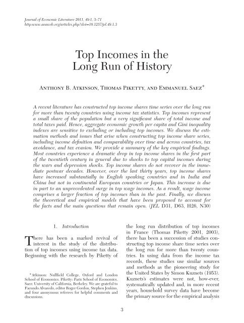
Atk<strong>in</strong>son, Piketty, <strong>and</strong> Saez: <strong>Top</strong> <strong>Incomes</strong> <strong>in</strong> <strong>the</strong> <strong>Long</strong> <strong>Run</strong> <strong>of</strong> History725%Share <strong>of</strong> total <strong>in</strong>come accru<strong>in</strong>g to each group20%15%10%5%0%<strong>Top</strong> 1% (<strong>in</strong>comes above $398,900 <strong>in</strong> 2007)<strong>Top</strong> 5–1% (<strong>in</strong>comes between $155,400 <strong>and</strong> $398,900)<strong>Top</strong> 10–5% (<strong>in</strong>comes between $109,600 <strong>and</strong> $155,400)1913191819231928193319381943194819531958196319681973197819831988199319982003Figure 2. Decompos<strong>in</strong>g <strong>the</strong> <strong>Top</strong> Decile US Income Share <strong>in</strong>to three Groups, 1913–2007Notes: Income is def<strong>in</strong>ed as market <strong>in</strong>come <strong>in</strong>clud<strong>in</strong>g capital ga<strong>in</strong>s (excludes all government transfers).<strong>Top</strong> 1 percent denotes <strong>the</strong> top percentile (families <strong>with</strong> annual <strong>in</strong>come above $398,900 <strong>in</strong> 2007).<strong>Top</strong> 5–1 percent denotes <strong>the</strong> next 4 percent (families <strong>with</strong> annual <strong>in</strong>come between $155,400 <strong>and</strong> $398,900 <strong>in</strong> 2007).<strong>Top</strong> 10–5 percent denotes <strong>the</strong> next 5 percent (bottom half <strong>of</strong> <strong>the</strong> top decile, families <strong>with</strong> annual <strong>in</strong>come between$109,600 <strong>and</strong> $155,400 <strong>in</strong> 2007).Source: Piketty <strong>and</strong> Saez (2003), series updated to 2007.<strong>in</strong> <strong>the</strong> pre–Great Depression era, wages <strong>and</strong>salaries now form a much greater fraction <strong>of</strong>top <strong>in</strong>comes than <strong>in</strong> <strong>the</strong> past.Why do <strong>the</strong>se <strong>in</strong>creases at <strong>the</strong> top matter?Several answers can be given. The mostgeneral is that people have a sense <strong>of</strong> fairness<strong>and</strong> care about <strong>the</strong> distribution <strong>of</strong> economicresources across <strong>in</strong>dividuals <strong>in</strong> society. As aresult, all advanced economies have set <strong>in</strong>place redistributive policies such as taxation—<strong>and</strong> <strong>in</strong> particular progressive taxation, <strong>and</strong>transfer programs, which effectively redistributea significant share <strong>of</strong> National Productacross <strong>in</strong>come groups. Importantly, differentparts <strong>of</strong> <strong>the</strong> distribution are <strong>in</strong>terdependent.Here we consider three more specific economicreasons why we should be <strong>in</strong>terested <strong>in</strong><strong>the</strong> top <strong>in</strong>come groups: <strong>the</strong>ir impact on overallgrowth <strong>and</strong> resources, <strong>the</strong>ir impact on overall<strong>in</strong>equality, <strong>and</strong> <strong>the</strong>ir global significance.2.1 Impact on Overall Growth <strong>and</strong>ResourcesThe textbook def<strong>in</strong>ition <strong>of</strong> <strong>in</strong>come by economistsrefers to “comm<strong>and</strong> over resources.”Are however <strong>the</strong> rich sufficiently numerous<strong>and</strong> sufficiently <strong>in</strong> receipt <strong>of</strong> <strong>in</strong>come that<strong>the</strong>y make an appreciable difference to <strong>the</strong>
8Journal <strong>of</strong> Economic Literature, Vol. XLIX (March 2011)12%10%Capital Ga<strong>in</strong>sCapital IncomeBus<strong>in</strong>ess IncomeSalaries8%6%4%2%0%1916192119261931193619411946195119561961196619711976198119861991199620012006Figure 3. The <strong>Top</strong> 0.1 Percent Income Share <strong>and</strong> Composition, 1916–2007Notes: The figure displays <strong>the</strong> top 0.1 percent <strong>in</strong>come share <strong>and</strong> its composition. Income is def<strong>in</strong>ed as market<strong>in</strong>come <strong>in</strong>clud<strong>in</strong>g capital ga<strong>in</strong>s (excludes all government transfers). Salaries <strong>in</strong>clude wages <strong>and</strong> salaries, bonus,exercised stock-options, <strong>and</strong> pensions. Bus<strong>in</strong>ess <strong>in</strong>come <strong>in</strong>cludes pr<strong>of</strong>its from sole proprietorships, partnerships,<strong>and</strong> S-corporations. Capital <strong>in</strong>come <strong>in</strong>cludes <strong>in</strong>terest <strong>in</strong>come, dividends, rents, royalties, <strong>and</strong> fiduciary <strong>in</strong>come.Capital ga<strong>in</strong>s <strong>in</strong>cludes realized capital ga<strong>in</strong>s net <strong>of</strong> losses.Source: Piketty <strong>and</strong> Saez (2003), series updated to 2007.overall control <strong>of</strong> resources? First, although<strong>the</strong> top 1 percent is by def<strong>in</strong>ition only a smallshare <strong>of</strong> <strong>the</strong> population, it does capture morethan a fifth <strong>of</strong> total <strong>in</strong>come—23.5 percent<strong>in</strong> <strong>the</strong> United States as <strong>of</strong> 2007. Second<strong>and</strong> even more important, <strong>the</strong> surge <strong>in</strong> top<strong>in</strong>comes over <strong>the</strong> last thirty years has a dramaticimpact on measured economic growth.As shown <strong>in</strong> table 1, U.S. real <strong>in</strong>come perfamily grew at a modest 1.2 percent annualrate from 1976 to 2007. However, whenexclud<strong>in</strong>g <strong>the</strong> top 1 percent, <strong>the</strong> average real<strong>in</strong>come <strong>of</strong> <strong>the</strong> bottom 99 percent grew at anannual rate <strong>of</strong> only 0.6 percent, which impliesthat <strong>the</strong> top 1 percent captured 58 percent<strong>of</strong> real economic growth per family dur<strong>in</strong>gthat period (column 4 <strong>in</strong> table 1). The effects<strong>of</strong> <strong>the</strong> top 1 percent on growth can be seeneven more dramatically <strong>in</strong> two contrast<strong>in</strong>grecent periods <strong>of</strong> economic expansion,1993–2000 (Cl<strong>in</strong>ton adm<strong>in</strong>istration expansion)<strong>and</strong> 2002–07 (Bush adm<strong>in</strong>istrationexpansion). Table 1 shows that, dur<strong>in</strong>g bo<strong>the</strong>xpansions, <strong>the</strong> real <strong>in</strong>comes <strong>of</strong> <strong>the</strong> top 1 percentgrew extremely quickly at an annualrate over 10.1 <strong>and</strong> 10.3 percent respectively.However, while <strong>the</strong> bottom 99 percent <strong>of</strong><strong>in</strong>comes grew at a solid pace <strong>of</strong> 2.7 percentper year from 1993 to 2000, <strong>the</strong>se <strong>in</strong>comesgrew only 1.3 percent per year from 2002
Atk<strong>in</strong>son, Piketty, <strong>and</strong> Saez: <strong>Top</strong> <strong>Incomes</strong> <strong>in</strong> <strong>the</strong> <strong>Long</strong> <strong>Run</strong> <strong>of</strong> History9Table 1<strong>Top</strong> Percentile Share <strong>and</strong> Average Income Growth <strong>in</strong> <strong>the</strong> United StatesAverage <strong>in</strong>comereal annualgrowth<strong>Top</strong> 1%<strong>in</strong>comes realannual growthBottom 99%<strong>in</strong>comes realannual growthFraction <strong>of</strong> totalgrowth captured bytop 1%(1) (2) (3) (4)Period1976–2007 1.2% 4.4% 0.6% 58%Cl<strong>in</strong>ton expansion1993–2000 4.0% 10.3% 2.7% 45%Bush expansion2002–2007 3.0% 10.1% 1.3% 65%Notes: Computations based on family market <strong>in</strong>come <strong>in</strong>clud<strong>in</strong>g realized capital ga<strong>in</strong>s (before <strong>in</strong>dividual taxes).<strong>Incomes</strong> are deflated us<strong>in</strong>g <strong>the</strong> Consumer Price Index (<strong>and</strong> us<strong>in</strong>g <strong>the</strong> CPI-U-RS before 1992). Column (4) reports<strong>the</strong> fraction <strong>of</strong> total real family <strong>in</strong>come growth captured by <strong>the</strong> top 1 percent. For example, from 2002 to 2007,average real family <strong>in</strong>comes grew by 3.0 percent annually but 65 percent <strong>of</strong> that growth accrued to <strong>the</strong> top 1percent while only 35 percent <strong>of</strong> that growth accrued to <strong>the</strong> bottom 99 percent <strong>of</strong> U.S. families.Source: Piketty <strong>and</strong> Saez (2003), series updated to 2007 <strong>in</strong> August 2009 us<strong>in</strong>g f<strong>in</strong>al IRS tax statistics.to 2007. Therefore, <strong>in</strong> <strong>the</strong> economic expansion<strong>of</strong> 2002–07, <strong>the</strong> top 1 percent capturedover two-thirds (65 percent) <strong>of</strong> <strong>in</strong>comegrowth. Those results may help expla<strong>in</strong> <strong>the</strong>gap between <strong>the</strong> economic experiences <strong>of</strong><strong>the</strong> public <strong>and</strong> <strong>the</strong> solid macroeconomicgrowth posted by <strong>the</strong> U.S. economy from2002 to <strong>the</strong> peak <strong>of</strong> 2007. Those results mayalso help expla<strong>in</strong> why <strong>the</strong> dramatic growth<strong>in</strong> top <strong>in</strong>comes dur<strong>in</strong>g <strong>the</strong> Cl<strong>in</strong>ton adm<strong>in</strong>istrationdid not generate much public outcrywhile <strong>the</strong>re has been an extraord<strong>in</strong>ary level<strong>of</strong> attention to top <strong>in</strong>comes <strong>in</strong> <strong>the</strong> U.S. press<strong>and</strong> <strong>in</strong> <strong>the</strong> public debate <strong>in</strong> recent years.Such changes also matter <strong>in</strong> <strong>in</strong>ternationalcomparisons. For example, average real<strong>in</strong>comes per family <strong>in</strong> <strong>the</strong> United States grewby 32.2 percent from 1975 to 2006 while <strong>the</strong>ygrew only by 27.1 percent <strong>in</strong> France dur<strong>in</strong>g<strong>the</strong> same period (Piketty 2001 <strong>and</strong> CamilleL<strong>and</strong>ais 2007), show<strong>in</strong>g that <strong>the</strong> macroeconomicperformance <strong>in</strong> <strong>the</strong> United Stateswas better than <strong>the</strong> French one dur<strong>in</strong>g thisperiod. Exclud<strong>in</strong>g <strong>the</strong> top percentile, averageU.S. real <strong>in</strong>comes grew only 17.9 percentdur<strong>in</strong>g <strong>the</strong> period while average French real<strong>in</strong>comes—exclud<strong>in</strong>g <strong>the</strong> top percentile—stillgrew at much <strong>the</strong> same rate (26.4 percent) asfor <strong>the</strong> whole French population. Therefore,<strong>the</strong> better macroeconomic performance <strong>of</strong><strong>the</strong> United States versus France is reversedwhen exclud<strong>in</strong>g <strong>the</strong> top 1 percent. 3More concretely, we can ask whe<strong>the</strong>r<strong>in</strong>creased taxes on <strong>the</strong> top <strong>in</strong>come groupwould yield appreciable revenue that couldbe deployed to fund public goods or redistribution?This question is <strong>of</strong> particular <strong>in</strong>terest<strong>in</strong> <strong>the</strong> current U.S. policy debate wherelarge government deficits will require rais<strong>in</strong>gtax revenue <strong>in</strong> com<strong>in</strong>g years. The st<strong>and</strong>ard3 It is important to note that such <strong>in</strong>ternational growthcomparisons are sensitive to <strong>the</strong> exact choice <strong>of</strong> yearscompared, <strong>the</strong> price deflator used, <strong>the</strong> exact def<strong>in</strong>ition<strong>of</strong> <strong>in</strong>come <strong>in</strong> each country, <strong>and</strong> hence are primarilyillustrative.
10Journal <strong>of</strong> Economic Literature, Vol. XLIX (March 2011)response by many economists <strong>in</strong> <strong>the</strong> past hasbeen that “<strong>the</strong> game is not worth <strong>the</strong> c<strong>and</strong>le.”Indeed, net <strong>of</strong> all federal taxes, <strong>in</strong> <strong>the</strong> UnitedStates <strong>in</strong> 1976 <strong>the</strong> top percentile receivedonly 5.8 percent <strong>of</strong> total pretax <strong>in</strong>come, anamount equal to 24 percent <strong>of</strong> all federal taxes(<strong>in</strong>dividual, corporate, estate taxes, <strong>and</strong> socialsecurity <strong>and</strong> health contributions) <strong>in</strong> that year.However, by 2007, net <strong>of</strong> all federal taxes,<strong>the</strong> top percentile received 17.3 percent <strong>of</strong>total pretax <strong>in</strong>come, or about 74 percent <strong>of</strong> allfederal taxes raised <strong>in</strong> 2007. 4 Therefore, it isclear that <strong>the</strong> surge <strong>in</strong> <strong>the</strong> top percentile sharehas greatly <strong>in</strong>creased <strong>the</strong> “tax capacity” at <strong>the</strong>top <strong>of</strong> <strong>the</strong> <strong>in</strong>come distribution. In budgetaryterms, this cannot be ignored. 52.2 Impact on Overall InequalityIt might be thought that top shares havelittle impact on overall <strong>in</strong>equality. If we drawa Lorenz curve, def<strong>in</strong>ed as <strong>the</strong> share <strong>of</strong> total<strong>in</strong>come accru<strong>in</strong>g to those below percentile p,as p goes from 0 (bottom <strong>of</strong> <strong>the</strong> distribution)to 100 (top <strong>of</strong> <strong>the</strong> distribution), <strong>the</strong>n <strong>the</strong> top 1percent would scarcely be dist<strong>in</strong>guishable on<strong>the</strong> horizontal axis from <strong>the</strong> vertical endpo<strong>in</strong>t,<strong>and</strong> <strong>the</strong> top 0.1 percent even less so. The mostcommonly used summary measure <strong>of</strong> overall<strong>in</strong>equality, <strong>the</strong> G<strong>in</strong>i coefficient, is more sensitiveto transfers at <strong>the</strong> center <strong>of</strong> <strong>the</strong> distributionthan at <strong>the</strong> tails. (The G<strong>in</strong>i coefficient isdef<strong>in</strong>ed as <strong>the</strong> ratio <strong>of</strong> <strong>the</strong> area between <strong>the</strong>Lorenz curve <strong>and</strong> <strong>the</strong> l<strong>in</strong>e <strong>of</strong> equality over <strong>the</strong>total area under <strong>the</strong> l<strong>in</strong>e <strong>of</strong> equality.)4 The 5.8 percent <strong>and</strong> 17.3 percent figures are based onaverage tax rates by <strong>in</strong>come groups presented <strong>in</strong> Piketty<strong>and</strong> Saez (2006). We exclude <strong>the</strong> corporate tax <strong>and</strong> <strong>the</strong>employer portion <strong>of</strong> payroll taxes as <strong>the</strong> pretax <strong>in</strong>comeshare series are based on market <strong>in</strong>come after corporatetaxes <strong>and</strong> employer payroll taxes. We have 5.8 percent= 8.8 percent * (1 − 0.262 − 0.016/2 − .068) <strong>and</strong>17.3 percent = 23.5 percent * (1 − .225 − 0.03/2 − 0.022).The percentage <strong>of</strong> all federal taxes is obta<strong>in</strong>ed us<strong>in</strong>g totalfederal average tax rates that are 24.7 percent <strong>and</strong> 23.7 percent<strong>in</strong> 1976 <strong>and</strong> 2007 from Piketty <strong>and</strong> Saez (2006).5 We discuss <strong>the</strong> important issue <strong>of</strong> <strong>the</strong> behavioralresponses <strong>of</strong> top <strong>in</strong>comes to taxes <strong>in</strong> section 5.But top shares can materially affect overall<strong>in</strong>equality, as may be seen from <strong>the</strong> follow<strong>in</strong>gcalculation. If we treat <strong>the</strong> very top groupas <strong>in</strong>f<strong>in</strong>itesimal <strong>in</strong> numbers, but <strong>with</strong> a f<strong>in</strong>iteshare S * <strong>of</strong> total <strong>in</strong>come, <strong>the</strong>n, graphically,<strong>the</strong> Lorenz curve reaches 1 − S * just belowp = 100. As a result, <strong>the</strong> total G<strong>in</strong>i coefficientcan be approximated by S * + (1 − S * )G, where G is <strong>the</strong> G<strong>in</strong>i coefficient for <strong>the</strong>population exclud<strong>in</strong>g <strong>the</strong> top group (Atk<strong>in</strong>son2007b). This means that, if <strong>the</strong> G<strong>in</strong>i coefficientfor <strong>the</strong> rest <strong>of</strong> <strong>the</strong> population is 40 percent,<strong>the</strong>n a rise <strong>of</strong> 14 percentage po<strong>in</strong>ts <strong>in</strong> <strong>the</strong> topshare, as happened <strong>with</strong> <strong>the</strong> share <strong>of</strong> <strong>the</strong> top1 percent <strong>in</strong> <strong>the</strong> United States from 1976 to2006, causes a rise <strong>of</strong> 8.4 percentage po<strong>in</strong>ts <strong>in</strong><strong>the</strong> overall G<strong>in</strong>i. This is larger than <strong>the</strong> <strong>of</strong>ficialG<strong>in</strong>i <strong>in</strong>crease from 39.8 percent to 47.0 percentover <strong>the</strong> 1976–2006 period based on U.S.household <strong>in</strong>come <strong>in</strong> <strong>the</strong> Current PopulationSurvey (U.S. Census Bureau 2008, table A3). 62.3 <strong>Top</strong> <strong>Incomes</strong> <strong>in</strong> a Global PerspectiveThe analysis so far has considered <strong>the</strong> role<strong>of</strong> top <strong>in</strong>comes <strong>in</strong> a purely national context,but it is evident that <strong>the</strong> rich, or at least <strong>the</strong>super-rich, are global players. What howeveris <strong>the</strong>ir quantitative significance on a worldscale? Does it matter if <strong>the</strong> share <strong>of</strong> <strong>the</strong> top1 percent <strong>in</strong> <strong>the</strong> United States doubles? Thetop 1 percent <strong>in</strong> <strong>the</strong> United States constitutes1.5 million tax units. How do <strong>the</strong>y fit <strong>in</strong>to aworld <strong>of</strong> some 6 billion people? Accord<strong>in</strong>g to<strong>the</strong> estimates <strong>of</strong> Francois Bourguignon <strong>and</strong>Christian Morrisson (2002), <strong>the</strong> world G<strong>in</strong>icoefficient went from 61 percent <strong>in</strong> 1910 to64 percent <strong>in</strong> 1950 <strong>and</strong> <strong>the</strong>n to 65.7 percent<strong>in</strong> 1992, as displayed <strong>in</strong> figure 4 (full triangleseries, right y-axis). 7 How did <strong>the</strong> evolution <strong>of</strong>top <strong>in</strong>come shares <strong>in</strong> richer countries, which6 The relation between top shares <strong>and</strong> overall <strong>in</strong>equalityis explored fur<strong>the</strong>r by Leigh (2007).7 As spelled out <strong>in</strong> Bourguignon <strong>and</strong> Morrisson (2002),strong assumptions are required to obta<strong>in</strong> a worldwideG<strong>in</strong>i coefficient based on country level <strong>in</strong>equality statistics.
Atk<strong>in</strong>son, Piketty, <strong>and</strong> Saez: <strong>Top</strong> <strong>Incomes</strong> <strong>in</strong> <strong>the</strong> <strong>Long</strong> <strong>Run</strong> <strong>of</strong> History110.25%70%% <strong>of</strong> world <strong>with</strong> <strong>in</strong>come above 20 times world mean0.20%0.15%0.10%0.05%0.00%Fraction super richFraction super rich (from US)World G<strong>in</strong>i65%60%55%50%45%19101915192019251930193519401945195019551960196519701975198019851990Worldwide G<strong>in</strong>i coefficientFigure 4. The Globally Super Rich <strong>and</strong> Worldwide G<strong>in</strong>i, 1910–1992Sources: Fraction super rich series is def<strong>in</strong>ed as <strong>the</strong> fraction <strong>of</strong> citizens <strong>in</strong> <strong>the</strong> world <strong>with</strong> <strong>in</strong>come abovetwenty times <strong>the</strong> world mean. Estimated by Atk<strong>in</strong>son (2007) us<strong>in</strong>g Bourguignon <strong>and</strong> Morrisson (2002) series.Fraction super rich (from U.S.) series is def<strong>in</strong>ed as <strong>the</strong> number <strong>of</strong> U.S. citizens <strong>with</strong> <strong>in</strong>come above twenty times <strong>the</strong>world mean divided by <strong>the</strong> world citizens. Estimated by Atk<strong>in</strong>son (2007) us<strong>in</strong>g Bourguignon <strong>and</strong> Morrisson(2002) series. Worldwide G<strong>in</strong>i series is <strong>the</strong> G<strong>in</strong>i coefficient among world citizens estimated by Bourguigon<strong>and</strong> Morrisson (2002).fell dur<strong>in</strong>g <strong>the</strong> first part <strong>of</strong> <strong>the</strong> twentieth century<strong>and</strong> <strong>in</strong>creased sharply <strong>in</strong> some countries<strong>in</strong> recent decades, affect this picture?To address this question, Atk<strong>in</strong>son(2007b) def<strong>in</strong>es <strong>the</strong> “globally rich” as those<strong>with</strong> more than twenty times <strong>the</strong> meanworld <strong>in</strong>come, which <strong>in</strong> 1992 meant above$100,000. Atk<strong>in</strong>son uses <strong>the</strong> distribution <strong>of</strong><strong>in</strong>come among world citizens constructed byBourguignon <strong>and</strong> Morrisson (2002) comb<strong>in</strong>ed<strong>with</strong> a Pareto imputation for <strong>the</strong> top <strong>of</strong> <strong>the</strong>distribution 8 to estimate <strong>the</strong> number <strong>of</strong>8 The Pareto parameter is estimated us<strong>in</strong>g <strong>the</strong> ratio <strong>of</strong><strong>the</strong> top 5 percent <strong>in</strong>come share to <strong>the</strong> top decile <strong>in</strong>comeshare (see equation (4) below), both be<strong>in</strong>g reported <strong>in</strong>“globally rich.” In 1992, <strong>the</strong>re were an estimated7.4 million people <strong>with</strong> <strong>in</strong>comes abovethis level, more than a third <strong>of</strong> <strong>the</strong>m <strong>in</strong> <strong>the</strong>United States. They constituted 0.14 percent<strong>of</strong> <strong>the</strong> world population but received5.4 percent <strong>of</strong> total world <strong>in</strong>come. As shownon figure 4 (left y-axis), as a proportion <strong>of</strong> <strong>the</strong>world population, <strong>the</strong> globally rich fell from0.23 percent <strong>in</strong> 1910 to 0.1 percent <strong>in</strong> 1970,mirror<strong>in</strong>g <strong>the</strong> decl<strong>in</strong>e <strong>in</strong> top <strong>in</strong>come sharesrecorded <strong>in</strong> <strong>in</strong>dividual countries. Therefore,Bourguignon <strong>and</strong> Morrisson (2002). Because those top<strong>in</strong>come shares are <strong>of</strong>ten based on survey data (<strong>and</strong> nottax data), <strong>the</strong>y likely underestimate <strong>the</strong> magnitude <strong>of</strong> <strong>the</strong>changes at <strong>the</strong> very top.
12Journal <strong>of</strong> Economic Literature, Vol. XLIX (March 2011)although overall <strong>in</strong>equality among world citizens<strong>in</strong>creased, <strong>the</strong>re was a compression at<strong>the</strong> top <strong>of</strong> <strong>the</strong> world distribution. But from1970, we see a reversal <strong>and</strong> a rise <strong>in</strong> <strong>the</strong> proportion<strong>of</strong> globally rich above <strong>the</strong> 1950 level.The number <strong>of</strong> globally rich doubled <strong>in</strong> <strong>the</strong>United States between 1970 <strong>and</strong> 1992, whichaccounts for half <strong>of</strong> <strong>the</strong> worldwide <strong>in</strong>crease<strong>in</strong> <strong>the</strong> number <strong>of</strong> “globally rich” <strong>and</strong> hencemakes a perceptible difference to <strong>the</strong> worlddistribution.2.4 SummaryThere are a number <strong>of</strong> reasons for study<strong>in</strong>g<strong>the</strong> development <strong>of</strong> top <strong>in</strong>come shares.Underst<strong>and</strong><strong>in</strong>g <strong>the</strong> extent <strong>of</strong> <strong>in</strong>equality at<strong>the</strong> top <strong>and</strong> <strong>the</strong> relative importance <strong>of</strong> differentfactors lead<strong>in</strong>g to <strong>in</strong>creas<strong>in</strong>g top sharesis important <strong>in</strong> <strong>the</strong> design <strong>of</strong> public policy.Concern about <strong>the</strong> rise <strong>in</strong> top shares <strong>in</strong> a number<strong>of</strong> countries has led to proposals for highertop <strong>in</strong>come tax rates; o<strong>the</strong>r countries are consider<strong>in</strong>glimits on remuneration <strong>and</strong> bonuses.The global distribution is com<strong>in</strong>g under<strong>in</strong>creas<strong>in</strong>g scrut<strong>in</strong>y as globalization proceeds.3. Methodology <strong>and</strong> Limitations3.1 MethodologyThe value <strong>of</strong> <strong>the</strong> tax data lies <strong>in</strong> <strong>the</strong> factthat, early on, <strong>the</strong> tax authorities <strong>in</strong> mostcountries began to compile <strong>and</strong> publish tabulationsbased on <strong>the</strong> exhaustive set <strong>of</strong> <strong>in</strong>cometax returns. 9 These tabulations generallyreport for a large number <strong>of</strong> <strong>in</strong>come brackets<strong>the</strong> correspond<strong>in</strong>g number <strong>of</strong> taxpayers, aswell as <strong>the</strong>ir total <strong>in</strong>come <strong>and</strong> tax liability.They are usually broken down by <strong>in</strong>comesource: capital <strong>in</strong>come, wage <strong>in</strong>come, bus<strong>in</strong>ess<strong>in</strong>come, etc. Table 2 shows an example<strong>of</strong> such a table from <strong>the</strong> British super-taxdata for fiscal year 1911–12. These datawere used by Arthur L. Bowley (1914), butit was not until <strong>the</strong> pioneer<strong>in</strong>g contribution<strong>of</strong> Kuznets (1953) that researchers began tocomb<strong>in</strong>e <strong>the</strong> tax data <strong>with</strong> external estimates<strong>of</strong> <strong>the</strong> total population <strong>and</strong> <strong>the</strong> total <strong>in</strong>come toestimate top <strong>in</strong>come shares. 10The data <strong>in</strong> table 2 illustrate <strong>the</strong> threemethodological problems addressed <strong>in</strong> thissection when estimat<strong>in</strong>g top <strong>in</strong>come shares.The first is <strong>the</strong> need to relate <strong>the</strong> numberor persons to a control total to def<strong>in</strong>e howmany tax filers represent a given fractilesuch as <strong>the</strong> top percentile. In <strong>the</strong> case <strong>of</strong> <strong>the</strong>United K<strong>in</strong>gdom <strong>in</strong> 1911–12, only a verysmall fraction <strong>of</strong> <strong>the</strong> population is subject to<strong>the</strong> super-tax: less than 12,000 taxpayers out<strong>of</strong> a total population <strong>of</strong> over twenty milliontax units, i.e., not much more than 0.05 percent.The second issue concerns <strong>the</strong> def<strong>in</strong>ition<strong>of</strong> <strong>in</strong>come <strong>and</strong> <strong>the</strong> relation to an <strong>in</strong>comecontrol total used as <strong>the</strong> denom<strong>in</strong>ator <strong>in</strong> <strong>the</strong>top <strong>in</strong>come share estimation. The third problemis that, for much <strong>of</strong> <strong>the</strong> period, <strong>the</strong> onlydata available are tabulated by ranges so that<strong>in</strong>terpolation estimation is required. Microdata only exist <strong>in</strong> recent decades. Note alsothat <strong>the</strong> tabulated data vary considerably <strong>in</strong><strong>the</strong> number <strong>of</strong> ranges <strong>and</strong> <strong>the</strong> <strong>in</strong>formationprovided for each range. Different methodshave been used for <strong>in</strong>terpolation, such9 The first <strong>in</strong>come tax distribution published for <strong>the</strong>United K<strong>in</strong>gdom related to 1801 (see Josiah C. Stamp1916) but no fur<strong>the</strong>r figures on total <strong>in</strong>come are availablefor <strong>the</strong> n<strong>in</strong>eteenth century on account <strong>of</strong> <strong>the</strong> moveto a schedular system. The publication <strong>of</strong> regular U.K.distributional data only commenced <strong>with</strong> <strong>the</strong> <strong>in</strong>troduction<strong>of</strong> supertax <strong>in</strong> 1909. Distributional data were howeveralready by <strong>the</strong>n be<strong>in</strong>g produced <strong>in</strong> certa<strong>in</strong> parts <strong>of</strong> <strong>the</strong>British Empire. For example, <strong>in</strong> 1905, <strong>the</strong> State <strong>of</strong> Victoria(Australia) supplied a table <strong>of</strong> <strong>the</strong> distribution <strong>of</strong> <strong>in</strong>come<strong>in</strong> 1903 <strong>in</strong> response to a request for <strong>in</strong>formation from <strong>the</strong>U.K. government (House <strong>of</strong> Commons 1905, p. 233).10 Before Kuznets, U.S. tax statistics had been used primarilyto estimate Pareto parameters as this does not requireestimat<strong>in</strong>g total population <strong>and</strong> total <strong>in</strong>come controls (seebelow): see for example William L. Crum (1935), Norris O.Johnson (1935 <strong>and</strong> 1937), <strong>and</strong> Rufus S. Tucker (1938). Thedrawback is that Pareto parameters only capture dispersion<strong>of</strong> <strong>in</strong>comes <strong>in</strong> <strong>the</strong> top tail <strong>and</strong>—unlike top <strong>in</strong>come shares—do not relate top <strong>in</strong>comes to average <strong>in</strong>comes.
Atk<strong>in</strong>son, Piketty, <strong>and</strong> Saez: <strong>Top</strong> <strong>Incomes</strong> <strong>in</strong> <strong>the</strong> <strong>Long</strong> <strong>Run</strong> <strong>of</strong> History13Table 2Example <strong>of</strong> Income Tax Data: UK Super-Tax, 1911–12Income class Number <strong>of</strong> persons Total <strong>in</strong>come assessedAt leastbut less than£5,000 £10,000 7,767 £52,810,069£10,000 £15,000 2,055 £24,765,153£15,000 £20,000 798 £13,742,318£20,000 £25,000 437 £9,653,890£25,000 £35,000 387 £11,385,691£35,000 £45,000 188 £7,464,861£45,000 £55,000 106 £5,274,658£55,000 £65,000 56 £3,295,110£65,000 £75,000 37 £2,590,606£75,000 £100,000 56 £4,929,787£100,000 — 66 £12,183,724Total 11,953 £148,095,867Source: Annual Report <strong>of</strong> <strong>the</strong> Inl<strong>and</strong> Revenue for <strong>the</strong> Year 1913–14: table 140, p. 155.as <strong>the</strong> Pareto <strong>in</strong>terpolation discussed <strong>in</strong> <strong>the</strong>next subsection <strong>and</strong> <strong>the</strong> split histogram (seeAtk<strong>in</strong>son 2005).3.1.1 Pareto InterpolationThe basic data are <strong>in</strong> <strong>the</strong> form <strong>of</strong> groupedtabulations, as <strong>in</strong> table 2, where <strong>the</strong> <strong>in</strong>tervalsdo not <strong>in</strong> general co<strong>in</strong>cide <strong>with</strong> <strong>the</strong> percentagegroups <strong>of</strong> <strong>the</strong> population <strong>with</strong> which weare concerned (such as <strong>the</strong> top 1 percent).We have <strong>the</strong>refore to <strong>in</strong>terpolate <strong>in</strong> order toarrive at values for summary statistics such as<strong>the</strong> shares <strong>of</strong> total <strong>in</strong>come. Moreover, someauthors have extrapolated upwards <strong>in</strong>to <strong>the</strong>open upper <strong>in</strong>terval <strong>and</strong> downwards below<strong>the</strong> lowest range tabulated. The Pareto law fortop <strong>in</strong>comes is given by <strong>the</strong> follow<strong>in</strong>g (cumulative)distribution function F(y) for <strong>in</strong>come y:(1) 1 − F(y) = (k/y) α (k > 0, α > 1),where k <strong>and</strong> α are given parameters,α is called <strong>the</strong> Pareto parameter. Thecorrespond<strong>in</strong>g density function is givenby f (y) = αk α /y (1+α) . The key property<strong>of</strong> Pareto distributions is that <strong>the</strong> ratio <strong>of</strong>average <strong>in</strong>come y * (y) <strong>of</strong> <strong>in</strong>dividuals <strong>with</strong><strong>in</strong>come above y to y does not depend on <strong>the</strong><strong>in</strong>come threshold y:(2) y * (y) = [ ∫ z>y z f (z) dz ] / [ ∫ z>y f (z) dz ]= [∫ z>y dz/z α ]/[∫ z>y dz/z (1+α) ]= α y/(α − 1),i.e., y * (y)/y = β , <strong>with</strong> β = α/(α − 1).That is, if β = 2, <strong>the</strong> average <strong>in</strong>come <strong>of</strong><strong>in</strong>dividuals <strong>with</strong> <strong>in</strong>come above $100,000 is$200,000 <strong>and</strong> <strong>the</strong> average <strong>in</strong>come <strong>of</strong> <strong>in</strong>dividuals<strong>with</strong> <strong>in</strong>come above $1 million is $2 million.Intuitively, a higher β means a fatter uppertail <strong>of</strong> <strong>the</strong> distribution. From now on, werefer to β as <strong>the</strong> <strong>in</strong>verted Pareto coefficient.Throughout this paper, we choose to focus
14Journal <strong>of</strong> Economic Literature, Vol. XLIX (March 2011)Table 3Pareto-Lorenz α Coefficients versus Inverted-Pareto-Lorenz β Coefficientsα β = α/(α − 1) β α = β/(β − 1)1.10 11.00 1.50 3.001.30 4.33 1.60 2.671.50 3.00 1.70 2.431.70 2.43 1.80 2.251.90 2.11 1.90 2.112.00 2.00 2.00 2.002.10 1.91 2.10 1.912.30 1.77 2.20 1.832.50 1.67 2.30 1.773.00 1.50 2.40 1.714.00 1.33 2.50 1.675.00 1.25 3.00 1.5010.00 1.11 3.50 1.40Notes:(1) The “α” coefficient is <strong>the</strong> st<strong>and</strong>ard Pareto-Lorenz coefficient commonly used <strong>in</strong> power-law distribution formulas:1−F(y) = (A/y) α <strong>and</strong> f(y) = αA α /y 1+α (A>0, α>1, f(y) = density function, F(y) = distribution function,1−F(y) = proportion <strong>of</strong> population <strong>with</strong> <strong>in</strong>come above y). A higher coefficient α means a faster convergence <strong>of</strong><strong>the</strong> density toward zero, i.e., a less fat upper tail.(2) The “β” coefficient is def<strong>in</strong>ed as <strong>the</strong> ratio y*(y)/y, i.e., <strong>the</strong> ratio between <strong>the</strong> average <strong>in</strong>come y*(y) <strong>of</strong> <strong>in</strong>dividuals<strong>with</strong> <strong>in</strong>come above threshold y <strong>and</strong> <strong>the</strong> threshold y. The characteristic property <strong>of</strong> power laws is that this ratio isa constant, i.e., does not depend on <strong>the</strong> threshold y. Simple computations show that β = y*(y)/y = α/(α−1),<strong>and</strong> conversely α = β/(β−1).on <strong>the</strong> <strong>in</strong>verted Pareto coefficient β (whichhas more <strong>in</strong>tuitive economic appeal) ra<strong>the</strong>rthan <strong>the</strong> st<strong>and</strong>ard Pareto coefficient α. Notethat <strong>the</strong>re exists a one-to-one, monotonicallydecreas<strong>in</strong>g relationship between <strong>the</strong> α <strong>and</strong> βcoefficients, i.e., β = α/(α − 1) <strong>and</strong> α = β/(β − 1) (see table 3). 11Vilfredo Pareto (1896, 1896–1897), <strong>in</strong><strong>the</strong> 1890s us<strong>in</strong>g tax tabulations from Swisscantons, found that this law approximatesremarkably well <strong>the</strong> top tails <strong>of</strong> <strong>the</strong> <strong>in</strong>comeor wealth distributions. S<strong>in</strong>ce Pareto, raw11 Put differently, (β − 1) is <strong>the</strong> <strong>in</strong>verse <strong>of</strong> (α − 1).It should be noted that this is different from <strong>the</strong><strong>in</strong>verse-Pareto coefficient used by Lee C. Soltow (1969),although this too <strong>in</strong>creases as <strong>the</strong> tail becomes fatter.tabulations by brackets produced by taxadm<strong>in</strong>istrations have <strong>of</strong>ten been used to estimatePareto parameters. 12 A number <strong>of</strong> <strong>the</strong>top <strong>in</strong>come studies conclude that <strong>the</strong> Paretoapproximation works remarkably well today,<strong>in</strong> <strong>the</strong> sense that for a given country <strong>and</strong> agiven year, <strong>the</strong> β coefficient is fairly <strong>in</strong>variant<strong>with</strong> y. However a key difference <strong>with</strong> <strong>the</strong>early Pareto literature, which was implicitlylook<strong>in</strong>g for some universal stability <strong>of</strong> <strong>in</strong>come<strong>and</strong> wealth distributions, is that our much12 There also exists a volum<strong>in</strong>ous <strong>the</strong>oretical literaturetry<strong>in</strong>g to expla<strong>in</strong> why Pareto laws fit <strong>the</strong> top tails <strong>of</strong> <strong>in</strong>come<strong>and</strong> wealth distributions. We survey some <strong>of</strong> <strong>the</strong>se <strong>the</strong>oreticalmodels <strong>in</strong> section 5 below. Pareto laws have also beenapplied <strong>in</strong> several areas outside <strong>in</strong>come <strong>and</strong> wealth distribution(see, e.g., Xavier Gabaix 2009 for a recent survey).
Atk<strong>in</strong>son, Piketty, <strong>and</strong> Saez: <strong>Top</strong> <strong>Incomes</strong> <strong>in</strong> <strong>the</strong> <strong>Long</strong> <strong>Run</strong> <strong>of</strong> History15larger time span <strong>and</strong> geographical scopeallows us to document <strong>the</strong> fact that Paretocoefficients vary substantially over time <strong>and</strong>across countries.From this viewpo<strong>in</strong>t, one additionaladvantage <strong>of</strong> us<strong>in</strong>g <strong>the</strong> β coefficient is thata higher β coefficient generally meanslarger top <strong>in</strong>come shares <strong>and</strong> higher <strong>in</strong>come<strong>in</strong>equality (while <strong>the</strong> reverse is true <strong>with</strong><strong>the</strong> more commonly used α coefficient).For <strong>in</strong>stance, <strong>in</strong> <strong>the</strong> United States, <strong>the</strong> βcoefficient (estimated at <strong>the</strong> top percentilethreshold <strong>and</strong> exclud<strong>in</strong>g capital ga<strong>in</strong>s)<strong>in</strong>creased gradually from 1.69 <strong>in</strong> 1976 to2.89 <strong>in</strong> 2007 as top percentile <strong>in</strong>come sharesurged from 7.9 percent to 18.9 percent. 13In a country like France, where <strong>the</strong> β coefficienthas been stable around 1.65–1.75s<strong>in</strong>ce <strong>the</strong> 1970s, <strong>the</strong> top percentile <strong>in</strong>comeshare has also been stable around 7.5 percent–8.5percent, except at <strong>the</strong> very end <strong>of</strong><strong>the</strong> period. 14 In practice, we shall see that βcoefficients typically vary between 1.5 <strong>and</strong> 3:values around 1.5–1.8 <strong>in</strong>dicate low <strong>in</strong>equalityby historical st<strong>and</strong>ards (<strong>with</strong> top 1 percent<strong>in</strong>come shares typically between 5 percent<strong>and</strong> 10 percent), while values around orabove 2.5 <strong>in</strong>dicate very high <strong>in</strong>equality (<strong>with</strong>top 1 percent <strong>in</strong>come shares typically around15 percent–20 percent or higher). In <strong>the</strong>case <strong>of</strong> <strong>the</strong> United K<strong>in</strong>gdom <strong>in</strong> 1911–12, ahigh <strong>in</strong>equality country, one can easily computefrom table 2 that <strong>the</strong> average <strong>in</strong>come <strong>of</strong>taxpayers above £5,000 was £12,390, i.e., <strong>the</strong>β coefficient was equal to 2.48. 15In practice, it is possible to verify whe<strong>the</strong>rPareto (or split histogram) <strong>in</strong>terpolations areaccurate when large micro tax return data<strong>with</strong> over-sampl<strong>in</strong>g at <strong>the</strong> top are available asis <strong>the</strong> case <strong>in</strong> <strong>the</strong> United States s<strong>in</strong>ce 1960.Those direct comparisons show that errorsdue to <strong>in</strong>terpolations are typically very smallif <strong>the</strong> number <strong>of</strong> brackets is sufficiently large<strong>and</strong> if <strong>in</strong>come amounts are also reported. In<strong>the</strong> end, <strong>the</strong> error due to Pareto <strong>in</strong>terpolationis likely to be dwarfed by various adjustments<strong>and</strong> imputations required for mak<strong>in</strong>gseries homogeneous, or errors <strong>in</strong> <strong>the</strong> estimation<strong>of</strong> <strong>the</strong> <strong>in</strong>come control total (see below).3.1.2 Control Total for PopulationIn some countries, such as Canada, NewZeal<strong>and</strong> from 1963, or <strong>the</strong> United K<strong>in</strong>gdomfrom 1990, <strong>the</strong> tax unit is <strong>the</strong> <strong>in</strong>dividual.In that case, <strong>the</strong> natural control total is <strong>the</strong>adult population def<strong>in</strong>ed as all residents ator above a certa<strong>in</strong> age cut<strong>of</strong>f, <strong>and</strong> <strong>the</strong> toppercentile share will measure <strong>the</strong> share <strong>of</strong>total <strong>in</strong>come accru<strong>in</strong>g to <strong>the</strong> top percentile<strong>of</strong> adult <strong>in</strong>dividuals. In o<strong>the</strong>r countries, taxunits are families. In <strong>the</strong> United K<strong>in</strong>gdom,for example, <strong>the</strong> tax unit until 1990 wasdef<strong>in</strong>ed as a married couple liv<strong>in</strong>g toge<strong>the</strong>r,<strong>with</strong> dependent children (<strong>with</strong>out <strong>in</strong>dependent<strong>in</strong>come), or as a s<strong>in</strong>gle adult, <strong>with</strong>dependent children, or as a child <strong>with</strong> <strong>in</strong>dependent<strong>in</strong>come. The control total used byAtk<strong>in</strong>son (2005) for <strong>the</strong> U.K. population forthis period is <strong>the</strong> total number <strong>of</strong> peopleaged 15 <strong>and</strong> over m<strong>in</strong>us <strong>the</strong> number <strong>of</strong> marriedfemales. In <strong>the</strong> United States, marriedwomen can file tax separate returns, but <strong>the</strong>number is “fairly small (about 1 percent <strong>of</strong>all returns <strong>in</strong> 1998)” (Piketty <strong>and</strong> Saez 2003).Piketty <strong>and</strong> Saez <strong>the</strong>refore treat <strong>the</strong> data as13 When we <strong>in</strong>clude capital ga<strong>in</strong>s, <strong>the</strong> rise <strong>of</strong> <strong>the</strong> β coefficientis even more dramatic, from 1.82 <strong>in</strong> 1976 to 3.42<strong>in</strong> 2007.14 See Atk<strong>in</strong>son <strong>and</strong> Piketty (2007, 2010).15 The stability <strong>of</strong> β coefficients (for a given country <strong>and</strong>a given year) only holds for top <strong>in</strong>comes, typically <strong>with</strong><strong>in</strong><strong>the</strong> top percentile. For <strong>in</strong>comes below <strong>the</strong> top percentile,<strong>the</strong> β coefficient takes much higher values (for very small<strong>in</strong>comes it goes to <strong>in</strong>f<strong>in</strong>ity). With<strong>in</strong> <strong>the</strong> top percentile, <strong>the</strong> βcoefficient varies slightly, <strong>and</strong> falls for <strong>the</strong> very top <strong>in</strong>comes(at <strong>the</strong> level <strong>of</strong> <strong>the</strong> s<strong>in</strong>gle richest taxpayer, β is by def<strong>in</strong>itionequal to 1), but generally not before <strong>the</strong> top 0.1 percentor top 0.01 percent threshold. In <strong>the</strong> example <strong>of</strong> table 2,one can easily compute that <strong>the</strong> β coefficient gradually fallsfrom 2.48 at <strong>the</strong> £5,000 threshold to 2.28 at <strong>the</strong> £10,000threshold <strong>and</strong> 1.85 at <strong>the</strong> £100,000 threshold (<strong>with</strong> onlysixty-six taxpayers left).
16Journal <strong>of</strong> Economic Literature, Vol. XLIX (March 2011)relat<strong>in</strong>g to families <strong>and</strong> take as a control total<strong>the</strong> sum <strong>of</strong> married males <strong>and</strong> all nonmarried<strong>in</strong>dividuals aged 20 <strong>and</strong> over.What difference does it make to use <strong>the</strong><strong>in</strong>dividual unit versus <strong>the</strong> family unit? If wetreat all units as weighted equally (so couplesdo not count twice) <strong>and</strong> take total <strong>in</strong>come,<strong>the</strong>n <strong>the</strong> impact <strong>of</strong> mov<strong>in</strong>g from a couplebasedto an <strong>in</strong>dividual-based system dependson <strong>the</strong> jo<strong>in</strong>t distribution <strong>of</strong> <strong>in</strong>come. A usefulspecial case is where <strong>the</strong> marg<strong>in</strong>al distributionsare such that <strong>the</strong> upper tail is Pareto<strong>in</strong> form. Suppose first that all rich peopleare ei<strong>the</strong>r unmarried or have partners <strong>with</strong>zero <strong>in</strong>come. The number <strong>of</strong> <strong>in</strong>dividuals <strong>with</strong><strong>in</strong>comes <strong>in</strong> excess <strong>of</strong> $Y is <strong>the</strong> same as <strong>the</strong>number <strong>of</strong> families <strong>and</strong> <strong>the</strong>ir total <strong>in</strong>come is<strong>the</strong> same. The overall <strong>in</strong>come control total isunchanged but <strong>the</strong> total number <strong>of</strong> <strong>in</strong>dividualsexceeds <strong>the</strong> total number <strong>of</strong> tax units (bya factor written as (1 + m)). This means thatto locate <strong>the</strong> top p percent, we now need togo fur<strong>the</strong>r down <strong>the</strong> distribution, <strong>and</strong>, given<strong>the</strong> Pareto assumption, <strong>the</strong> share rises by afactor (1 + m) 1-1/α . With α = 2 <strong>and</strong> m = 0.4,this equals 1.18. On <strong>the</strong> o<strong>the</strong>r h<strong>and</strong>, if allrich tax units consist <strong>of</strong> couples <strong>with</strong> equal<strong>in</strong>comes, <strong>the</strong>n <strong>the</strong> same amount (<strong>and</strong> share)<strong>of</strong> total <strong>in</strong>come is received by 2/(1 + m) times<strong>the</strong> fraction <strong>of</strong> <strong>the</strong> population. In <strong>the</strong> case <strong>of</strong><strong>the</strong> Pareto distribution, this means that <strong>the</strong>share <strong>of</strong> <strong>the</strong> top 1 percent is reduced by afactor (2/(1 + m)) 1−1/α . With α = 2 <strong>and</strong>m = 0.4, this equals 1.2. We have <strong>the</strong>reforelikely bounds on <strong>the</strong> effect <strong>of</strong> mov<strong>in</strong>g to an<strong>in</strong>dividual basis. If <strong>the</strong> share <strong>of</strong> <strong>the</strong> top 1 percentis 10 percent, <strong>the</strong>n this could be <strong>in</strong>creasedto 11.8 percent or reduced to 8.3 percent. Thelocation <strong>of</strong> <strong>the</strong> actual figure between <strong>the</strong>sebounds depends on <strong>the</strong> jo<strong>in</strong>t distribution, <strong>and</strong>this may well have changed over <strong>the</strong> century.Saez <strong>and</strong> Michael R. Veall (2005), <strong>in</strong> <strong>the</strong>case <strong>of</strong> Canada, can compute top wage<strong>in</strong>come shares both on an <strong>in</strong>dividual <strong>and</strong>family base s<strong>in</strong>ce 1982. They f<strong>in</strong>d that <strong>in</strong>dividualbased top shares are slightly higher(by about 5 percent). Most importantly, <strong>the</strong>family based <strong>and</strong> <strong>in</strong>dividual based top sharestrack each o<strong>the</strong>r extremely closely. Similarly,Wojciech Kopczuk, Saez, <strong>and</strong> Jae Song(2010) compute <strong>in</strong>dividual based top wage<strong>in</strong>come shares <strong>and</strong> show that <strong>the</strong>y track alsovery closely <strong>the</strong> family based wage <strong>in</strong>comeshares estimated by Piketty <strong>and</strong> Saez (2003).This shows that changes <strong>in</strong> <strong>the</strong> correlation <strong>of</strong>earn<strong>in</strong>gs across spouses have played a negligiblerole <strong>in</strong> <strong>the</strong> surge <strong>in</strong> top wage <strong>in</strong>comeshares <strong>in</strong> North America. However, shift<strong>in</strong>gfrom family to <strong>in</strong>dividual units does have animpact on <strong>the</strong> level <strong>of</strong> top <strong>in</strong>come shares <strong>and</strong>creates a discont<strong>in</strong>uity <strong>in</strong> <strong>the</strong> series. 163.1.3 Control Total for IncomeThe aim is to relate <strong>the</strong> amounts recorded<strong>in</strong> <strong>the</strong> tax data (numerator <strong>of</strong> <strong>the</strong> top share) toa comparable control total for <strong>the</strong> full population(denom<strong>in</strong>ator <strong>of</strong> <strong>the</strong> top share). This isa matter that requires attention, s<strong>in</strong>ce differentmethods are employed, which may affectcomparability overtime <strong>and</strong> across countries.One approach starts from <strong>the</strong> <strong>in</strong>come tax data<strong>and</strong> adds <strong>the</strong> <strong>in</strong>come <strong>of</strong> those not covered (<strong>the</strong>“nonfilers”). This approach is used for examplefor <strong>the</strong> United K<strong>in</strong>gdom (Atk<strong>in</strong>son 2005), <strong>and</strong><strong>the</strong> United States (Piketty <strong>and</strong> Saez 2003) for<strong>the</strong> years s<strong>in</strong>ce 1944. The approach <strong>in</strong> effecttakes <strong>the</strong> def<strong>in</strong>ition <strong>of</strong> <strong>in</strong>come embodied <strong>in</strong><strong>the</strong> tax legislation, <strong>and</strong> <strong>the</strong> result<strong>in</strong>g estimateswill change <strong>with</strong> variations <strong>in</strong> <strong>the</strong> tax law. Forexample, short-term capital ga<strong>in</strong>s have been<strong>in</strong>cluded to vary<strong>in</strong>g degrees <strong>in</strong> taxable <strong>in</strong>come<strong>in</strong> <strong>the</strong> United K<strong>in</strong>gdom. A second approach,16 Most studies correct for such discont<strong>in</strong>uities by correct<strong>in</strong>gseries to elim<strong>in</strong>ate <strong>the</strong> discont<strong>in</strong>uity. Absent overlapp<strong>in</strong>gdata at both <strong>the</strong> family <strong>and</strong> <strong>in</strong>dividual levels, sucha correction has to be based on strong assumptions (forexample that <strong>the</strong> rate <strong>of</strong> growth <strong>in</strong> <strong>in</strong>come shares around<strong>the</strong> discont<strong>in</strong>uity is equal to <strong>the</strong> average rate <strong>of</strong> growth <strong>the</strong>year before <strong>and</strong> <strong>the</strong> year after <strong>the</strong> discont<strong>in</strong>uity). We flagstudies <strong>in</strong> table 4 where no correction for such discont<strong>in</strong>uitiesare made.
Atk<strong>in</strong>son, Piketty, <strong>and</strong> Saez: <strong>Top</strong> <strong>Incomes</strong> <strong>in</strong> <strong>the</strong> <strong>Long</strong> <strong>Run</strong> <strong>of</strong> History17pioneered by Kuznets (1953), starts from anexternal control total, typically derived from<strong>the</strong> national accounts. This approach is followedfor example <strong>in</strong> France (Piketty 2001,2003), or <strong>the</strong> United States for <strong>the</strong> years priorto 1944. The approach seeks to adjust <strong>the</strong> taxdata to <strong>the</strong> same basis, correct<strong>in</strong>g for examplefor miss<strong>in</strong>g <strong>in</strong>come <strong>and</strong> for differences<strong>in</strong> tim<strong>in</strong>g. In this case, <strong>the</strong> <strong>in</strong>come <strong>of</strong> nonfilersappears as a residual. This approach hasa firmer conceptual base, but <strong>the</strong>re are significantdifferences between <strong>in</strong>come conceptsused <strong>in</strong> national accounts <strong>and</strong> those used for<strong>in</strong>come tax purposes.The first approach estimates <strong>the</strong> total<strong>in</strong>come that would have been reported ifeverybody had been required to file a taxreturn. Requirements to file a tax return varyacross time <strong>and</strong> across countries. Typicallymost countries have moved from a situationat <strong>the</strong> beg<strong>in</strong>n<strong>in</strong>g <strong>of</strong> <strong>the</strong> last century when am<strong>in</strong>ority filed returns to a situation todaywhere <strong>the</strong> great majority are covered. Forexample, <strong>in</strong> <strong>the</strong> United States, “before 1944,because <strong>of</strong> large exemption levels, only asmall fraction <strong>of</strong> <strong>in</strong>dividuals had to file taxreturns” (Piketty <strong>and</strong> Saez 2003, p. 4). Itshould be noted that taxpayers might notneed to make a tax return to appear <strong>in</strong> <strong>the</strong>statistics. Where <strong>the</strong>re is tax collection atsource, as <strong>with</strong> Pay-As-You-Earn (PAYE) <strong>in</strong><strong>the</strong> United K<strong>in</strong>gdom, many people do notfile a tax return but are covered by <strong>the</strong> payrecords <strong>of</strong> <strong>the</strong>ir employers. Estimates <strong>of</strong> <strong>the</strong><strong>in</strong>come <strong>of</strong> nonfilers may be related to <strong>the</strong>average <strong>in</strong>come <strong>of</strong> filers. For <strong>the</strong> UnitedStates, Piketty <strong>and</strong> Saez (2003), for <strong>the</strong>period s<strong>in</strong>ce 1944, impute to nonfilers a fixedfraction equal to 20 percent <strong>of</strong> filers’ average<strong>in</strong>come. In some cases, estimates <strong>of</strong> <strong>the</strong><strong>in</strong>come <strong>of</strong> nonfilers already exist. Atk<strong>in</strong>son(2005) makes use <strong>of</strong> <strong>the</strong> work <strong>of</strong> <strong>the</strong> CentralStatistical Office for <strong>the</strong> United K<strong>in</strong>gdom.The second approach starts from <strong>the</strong>national accounts totals for personal <strong>in</strong>come.In <strong>the</strong> case <strong>of</strong> <strong>the</strong> United States, Piketty <strong>and</strong>Saez use, for <strong>the</strong> period 1913–43, a controltotal equal to 80 percent <strong>of</strong> (total personal<strong>in</strong>come less transfers). In Canada, Saez <strong>and</strong>Veall (2005) use this approach for <strong>the</strong> entireperiod 1920–2000. How do <strong>the</strong>se national<strong>in</strong>come based calculations relate to <strong>the</strong> totals<strong>in</strong> <strong>the</strong> tax data? In answer<strong>in</strong>g this question, itmay be helpful to bear <strong>in</strong> m<strong>in</strong>d <strong>the</strong> differentstages set out schematically below:Personal sector total <strong>in</strong>come (PI)m<strong>in</strong>us Nonhousehold <strong>in</strong>come (Nonpr<strong>of</strong>it<strong>in</strong>stitutions such as charities)equals Household sector total <strong>in</strong>comem<strong>in</strong>us Items not <strong>in</strong>cluded <strong>in</strong> tax base(e.g., employers’ social securitycontributions <strong>and</strong>—<strong>in</strong> some countries—employees’social securitycontributions, imputed rent onowner-occupied houses, <strong>and</strong> nontaxabletransfer payments)equals Household gross <strong>in</strong>come returnableto tax authoritiesm<strong>in</strong>us Taxable <strong>in</strong>come not declared byfilersm<strong>in</strong>us Taxable <strong>in</strong>come <strong>of</strong> those not<strong>in</strong>cluded <strong>in</strong> tax returns (“nonfilers”)equals Declared taxable <strong>in</strong>come <strong>of</strong> filers.The use <strong>of</strong> national accounts totals maybe seen as mov<strong>in</strong>g down from <strong>the</strong> top ra<strong>the</strong>rthan mov<strong>in</strong>g up from <strong>the</strong> bottom by add<strong>in</strong>g<strong>the</strong> estimated <strong>in</strong>come <strong>of</strong> nonfilers. The percentageformulae can be seen as correct<strong>in</strong>gfor <strong>the</strong> nonhousehold elements <strong>and</strong> for <strong>the</strong>difference between returnable <strong>in</strong>come <strong>and</strong><strong>the</strong> national accounts def<strong>in</strong>ition. Some <strong>of</strong> <strong>the</strong>items, such as social security contributions,can be substantial. Piketty <strong>and</strong> Saez base<strong>the</strong>ir choice <strong>of</strong> percentage for <strong>the</strong> UnitedStates on <strong>the</strong> experience for <strong>the</strong> period1944–98, when <strong>the</strong>y applied estimates <strong>of</strong> <strong>the</strong><strong>in</strong>come <strong>of</strong> nonfilers.Given <strong>the</strong> <strong>in</strong>creas<strong>in</strong>g significance <strong>of</strong> some<strong>of</strong> <strong>the</strong> items (such as employers’ contributions)<strong>and</strong> <strong>of</strong> <strong>the</strong> nonhousehold <strong>in</strong>stitutions
18Journal <strong>of</strong> Economic Literature, Vol. XLIX (March 2011)(such as pension funds), it is not evident thata constant percentage is appropriate. S<strong>in</strong>cetransfers were also smaller at <strong>the</strong> start <strong>of</strong> <strong>the</strong>twentieth century, total household returnable<strong>in</strong>come was <strong>the</strong>n closer to total personal<strong>in</strong>come. Atk<strong>in</strong>son (2007) compares <strong>the</strong> twomethods <strong>in</strong> <strong>the</strong> case <strong>of</strong> <strong>the</strong> United K<strong>in</strong>gdom.He shows that <strong>the</strong> total <strong>in</strong>come estimatedfrom <strong>the</strong> first method by estimat<strong>in</strong>g <strong>the</strong><strong>in</strong>come <strong>of</strong> nonfilers trends slightly downwardsrelative to personal <strong>in</strong>come m<strong>in</strong>ustransfers from around 90 percent <strong>in</strong> <strong>the</strong>first part <strong>of</strong> <strong>the</strong> twentieth century to around85 percent <strong>in</strong> <strong>the</strong> last part <strong>of</strong> <strong>the</strong> century.Fur<strong>the</strong>rmore, <strong>the</strong>re are substantial shorttermvariations especially dur<strong>in</strong>g world warepisodes when <strong>the</strong> national accounts figuresappear to be relatively higher by as much as15–20 percent. Some countries do not havedeveloped national accounts, especially <strong>in</strong><strong>the</strong> earlier periods covered by tax statistics.In that case, <strong>the</strong> total <strong>in</strong>come control is chosenas a fixed percentage <strong>of</strong> GDP where <strong>the</strong>percentage is calibrated us<strong>in</strong>g later periodswhen National accounts are more developed.Need for a control total for <strong>in</strong>come is <strong>of</strong>course avoided if we exam<strong>in</strong>e <strong>the</strong> “shares<strong>with</strong><strong>in</strong> shares” that depend solely on populationtotals <strong>and</strong> <strong>the</strong> <strong>in</strong>come distribution <strong>with</strong><strong>in</strong><strong>the</strong> top, measured by <strong>the</strong> Pareto coefficient.This gives a measure <strong>of</strong> <strong>the</strong> degree <strong>of</strong> <strong>in</strong>equalityamong <strong>the</strong> top <strong>in</strong>comes that may be morerobust but does not compare top <strong>in</strong>comes to<strong>the</strong> average as top <strong>in</strong>come shares do.3.1.4 Adjustments for Income Def<strong>in</strong>itionIn a number <strong>of</strong> cases, <strong>the</strong> def<strong>in</strong>ition <strong>of</strong><strong>in</strong>come used to present <strong>the</strong> tabulationschanges over time. To obta<strong>in</strong> homogeneousseries, such changes need to be correctedfor. The most common change <strong>in</strong> <strong>the</strong> presentation<strong>of</strong> tabulations is due to shifts from net<strong>in</strong>come (<strong>in</strong>come after deductions) to gross<strong>in</strong>come (<strong>in</strong>come before deductions). Whencomposition <strong>in</strong>formation on <strong>the</strong> amount <strong>of</strong>deductions by <strong>in</strong>come brackets is available,<strong>the</strong> series estimated can be corrected forsuch changes. If we assume that rank<strong>in</strong>g <strong>of</strong><strong>in</strong>dividuals by net <strong>in</strong>come <strong>and</strong> gross <strong>in</strong>comeare approximately <strong>the</strong> same, <strong>the</strong> correctioncan be made by simply add<strong>in</strong>g back averagedeductions bracket by bracket to go from net<strong>in</strong>comes to gross <strong>in</strong>comes. This assumptioncan be checked when micro-data is availableas is <strong>the</strong> case <strong>in</strong> <strong>the</strong> United States s<strong>in</strong>ce 1960for example (Piketty <strong>and</strong> Saez 2003).It is also <strong>of</strong> <strong>in</strong>terest to estimate both series<strong>in</strong>clud<strong>in</strong>g capital ga<strong>in</strong>s <strong>and</strong> series exclud<strong>in</strong>gcapital ga<strong>in</strong>s (see below). This can alsobe done if data on amounts <strong>of</strong> capital ga<strong>in</strong>sare available by <strong>in</strong>come brackets. Becausecapital ga<strong>in</strong>s can be quite important at <strong>the</strong>top (see figure 3), rank<strong>in</strong>g <strong>of</strong> <strong>in</strong>dividualsmight change significantly when <strong>in</strong>clud<strong>in</strong>g orexclud<strong>in</strong>g capital ga<strong>in</strong>s. The ideal is <strong>the</strong>reforeto have access to micro-data to create tabulationsboth <strong>in</strong>clud<strong>in</strong>g <strong>and</strong> exclud<strong>in</strong>g capitalga<strong>in</strong>s. The micro-data can also be used toassess how rank<strong>in</strong>g changes when exclud<strong>in</strong>gcapital ga<strong>in</strong>s <strong>and</strong> hence develop simple rules<strong>of</strong> thumb to construct series exclud<strong>in</strong>g capitalga<strong>in</strong>s when start<strong>in</strong>g <strong>with</strong> series <strong>in</strong>clud<strong>in</strong>gcapital ga<strong>in</strong>s (or vice versa). This is done <strong>in</strong>Piketty <strong>and</strong> Saez (2003) for <strong>the</strong> period before1960, <strong>the</strong> first year when micro-data becomeavailable <strong>in</strong> <strong>the</strong> United States.3.1.5 O<strong>the</strong>r StudiesAs mentioned above, Kuznets (1953)developed <strong>the</strong> methodology <strong>of</strong> comb<strong>in</strong><strong>in</strong>gnational accounts <strong>with</strong> tax statistics to estimatetop <strong>in</strong>come shares. Before Kuznets,studies us<strong>in</strong>g tax statistics were limited to<strong>the</strong> estimation <strong>of</strong> Pareto parameters (start<strong>in</strong>g<strong>with</strong> Pareto 1896 <strong>and</strong> followed by numerousstudies across many countries <strong>and</strong> time periods)or to situations where <strong>the</strong> coverage <strong>of</strong>tax statistics was substantial or could be supplemented<strong>with</strong> additional <strong>in</strong>come data (as<strong>in</strong> Sc<strong>and</strong><strong>in</strong>avian countries, <strong>the</strong> Ne<strong>the</strong>rl<strong>and</strong>s,<strong>the</strong> German states, or <strong>the</strong> United K<strong>in</strong>gdomas we mentioned above). Therefore, <strong>the</strong>re
Atk<strong>in</strong>son, Piketty, <strong>and</strong> Saez: <strong>Top</strong> <strong>Incomes</strong> <strong>in</strong> <strong>the</strong> <strong>Long</strong> <strong>Run</strong> <strong>of</strong> History19exist a number <strong>of</strong> older studies <strong>in</strong> thosecountries comput<strong>in</strong>g top <strong>in</strong>come shares fromtax statistics. In general, those studies arelimited to a few years. Those studies are surveyed<strong>in</strong> L<strong>in</strong>dert (2000) for <strong>the</strong> United States<strong>and</strong> <strong>the</strong> United K<strong>in</strong>gdom <strong>and</strong> Morrisson(2000) for Europe. They are also discussed <strong>in</strong>each modern study country by country. Wemention <strong>the</strong> most important <strong>of</strong> those studiesat <strong>the</strong> bottom <strong>of</strong> table 4. The only countryfor which no modern study exists <strong>and</strong> olderstudies exist is Denmark. Those studies forDenmark show that top <strong>in</strong>comes shares fellsubstantially (as <strong>in</strong> o<strong>the</strong>r Nordic countries) <strong>in</strong><strong>the</strong> first half <strong>of</strong> <strong>the</strong> twentieth century till atleast 1963 (Rewal Schmidt Sorensen 1993).We also mention <strong>in</strong> table 4 o<strong>the</strong>r importantrecent country specific contributions, <strong>in</strong>clud<strong>in</strong>gthose by Joachim Merz, Dierk Hirschel,<strong>and</strong> Markus Zwick (2005) <strong>and</strong> by StefanBach, Giacomo Corneo, <strong>and</strong> Viktor Ste<strong>in</strong>er(2008) <strong>of</strong> Germany, by Bjorn Gustafsson <strong>and</strong>Birgitta Jansson (2007) <strong>of</strong> Sweden, <strong>and</strong> byJordi Guilera Rafecas (2008) <strong>of</strong> Portugal. 17Table 4 provides a syn<strong>the</strong>tic summary <strong>of</strong><strong>the</strong> key features <strong>of</strong> <strong>the</strong> estimates for all <strong>the</strong>studies to date. It should be noted that <strong>the</strong>table refers, <strong>in</strong> some cases, to testimatesupdat<strong>in</strong>g those <strong>in</strong> <strong>the</strong> published studies.3.2 Possible Limitations<strong>Top</strong> <strong>in</strong>come share series are constructedus<strong>in</strong>g tax statistics. The use <strong>of</strong> tax data is <strong>of</strong>tenregarded by economists <strong>with</strong> considerabledisbelief. In <strong>the</strong> United K<strong>in</strong>gdom, Richard M.Titmuss wrote <strong>in</strong> 1962 a book-length critique<strong>of</strong> <strong>the</strong> <strong>in</strong>come tax-based statistics on distribution,conclud<strong>in</strong>g, “we are expect<strong>in</strong>g too muchfrom <strong>the</strong> crumbs that fall from <strong>the</strong> conven-17 This survey does not cover <strong>the</strong> estimates for formerBritish colonial territories be<strong>in</strong>g prepared as part <strong>of</strong> a projectbe<strong>in</strong>g carried out by Atk<strong>in</strong>son (apart from S<strong>in</strong>gapore,shown <strong>in</strong> table 4). This project has assembled data for someforty former colonies cover<strong>in</strong>g <strong>the</strong> periods before <strong>and</strong> after<strong>in</strong>dependence. Data for French colonies <strong>and</strong> Brazil arebe<strong>in</strong>g exam<strong>in</strong>ed by Facundo Alvaredo.tional tables” (p. 191). More recently, compilers<strong>of</strong> databases on <strong>in</strong>come <strong>in</strong>equality havetended to rely on household survey data, dismiss<strong>in</strong>g<strong>in</strong>come tax data as unrepresentative.These doubts are well justified for at least tworeasons. The first is that tax data are collectedas part <strong>of</strong> an adm<strong>in</strong>istrative process, which isnot tailored to our needs, so that <strong>the</strong> def<strong>in</strong>ition<strong>of</strong> <strong>in</strong>come, <strong>of</strong> <strong>in</strong>come unit, etc. are not necessarilythose that we would have chosen. Thiscauses particular difficulties for comparisonsacross countries, but also for time-series analysiswhere <strong>the</strong>re have been substantial changes<strong>in</strong> <strong>the</strong> tax system, such as <strong>the</strong> moves to <strong>and</strong>from <strong>the</strong> jo<strong>in</strong>t taxation <strong>of</strong> couples. Secondly, itis obvious that those pay<strong>in</strong>g tax have a f<strong>in</strong>ancial<strong>in</strong>centive to present <strong>the</strong>ir affairs <strong>in</strong> a waythat reduces tax liabilities. There is tax avoidance<strong>and</strong> tax evasion. The rich, <strong>in</strong> particular,have a strong <strong>in</strong>centive to understate <strong>the</strong>irtaxable <strong>in</strong>comes. Those <strong>with</strong> wealth take stepsto ensure that <strong>the</strong> return comes <strong>in</strong> <strong>the</strong> form<strong>of</strong> asset appreciation, typically taxed at lowerrates or not at all. Those <strong>with</strong> high salariesseek to ensure that part <strong>of</strong> <strong>the</strong>ir remunerationcomes <strong>in</strong> forms, such as fr<strong>in</strong>ge benefits or stockoptions, that receive favorable tax treatment.Both groups may make use <strong>of</strong> tax havens thatallow <strong>in</strong>come to be moved beyond <strong>the</strong> reach<strong>of</strong> <strong>the</strong> national tax net. Third, <strong>the</strong> tax data is<strong>in</strong> general silent about <strong>the</strong> <strong>in</strong>dustrial composition<strong>of</strong> top <strong>in</strong>comes, which limits our abilityto <strong>in</strong>terpret <strong>and</strong> underst<strong>and</strong> changes. It wouldbe good, for example, to know more about <strong>the</strong>l<strong>in</strong>ks between ris<strong>in</strong>g top <strong>in</strong>come shares <strong>and</strong>Information <strong>and</strong> Communication Technologies(ICT), but this requires o<strong>the</strong>r data.These shortcom<strong>in</strong>gs limit what can be saidfrom tax data but this does not mean that <strong>the</strong>data are worthless. Like all economic data,<strong>the</strong>y measure <strong>with</strong> error <strong>the</strong> “true” variable<strong>in</strong> which we are <strong>in</strong>terested. As <strong>with</strong> all data,<strong>the</strong>re are potential sources <strong>of</strong> bias but, as <strong>in</strong>o<strong>the</strong>r cases, we can say someth<strong>in</strong>g about <strong>the</strong>possible direction <strong>and</strong> magnitude <strong>of</strong> <strong>the</strong> bias.Moreover, we can compensate for some <strong>of</strong> <strong>the</strong>
20Journal <strong>of</strong> Economic Literature, Vol. XLIX (March 2011)Table 4Key Features <strong>of</strong> Estimates for Each CountryFrance United K<strong>in</strong>gdom United States Canada AustraliaReferences Piketty (2001,2003)L<strong>and</strong>ais (2007)Atk<strong>in</strong>son(2005, 2007a)Piketty <strong>and</strong> Saez(2003)Saez <strong>and</strong> Veall(2005)Atk<strong>in</strong>son <strong>and</strong> Leigh(2007a)Yearscovered1900–20061900–1910aggregate,(1911–1914miss<strong>in</strong>g)(92 years)1908–2005.(1961 <strong>and</strong> 1980miss<strong>in</strong>g)(95 years)1913–2007(96 years)1920–2000(81 years)1921–2002 (plusState <strong>of</strong> Victoria for1912–1923)(82 years)InitialcoverageInitially under5%Initially only top0.05%Initially onlyaround 1%Initiallyaround 5%Initiallyaround 10%Unit <strong>of</strong>analysisPopulationdef<strong>in</strong>itionFamily Family to 1989;<strong>in</strong>dividual from1990Total number <strong>of</strong>familiescalculated fromnumber <strong>of</strong>households <strong>and</strong>household compositiondataAged 15 <strong>and</strong>over; before1990 total number<strong>of</strong> taxunits calculatedfrom populationaged 15 <strong>and</strong> overm<strong>in</strong>us number <strong>of</strong>married womenFamily Individual IndividualTotal number <strong>of</strong>families calculatedas marriedmen plus nonmarried men<strong>and</strong> women aged20 <strong>and</strong> overAged 20 <strong>and</strong>overAged 15 <strong>and</strong>overMethod <strong>of</strong>calculat<strong>in</strong>gcontrol totalsfor <strong>in</strong>comeFrom nationalaccountsAddition <strong>of</strong>estimated<strong>in</strong>come <strong>of</strong>nonfilersFrom 1944,addition <strong>of</strong><strong>in</strong>come <strong>of</strong>nonfilers = 20%average <strong>in</strong>come;before 1944 80%(personal <strong>in</strong>come—transfers)from nationalaccounts80% (personal<strong>in</strong>come—transfers)fromnationalaccountsTotal <strong>in</strong>comeconstructedfrom nationalaccountsIncomedef<strong>in</strong>itionGross <strong>in</strong>come,net <strong>of</strong> employeesocial securitycontributionsPrior to 1975<strong>in</strong>come net <strong>of</strong>certa<strong>in</strong>deductions;from 1975 total<strong>in</strong>comeGross <strong>in</strong>come,adjusted for net<strong>in</strong>comedeductionsGross <strong>in</strong>come,adjusted for <strong>the</strong>gross<strong>in</strong>g up <strong>of</strong>dividend <strong>in</strong>comeActual gross<strong>in</strong>come; adjustmentmade to taxable<strong>in</strong>come priorto 1957
Atk<strong>in</strong>son, Piketty, <strong>and</strong> Saez: <strong>Top</strong> <strong>Incomes</strong> <strong>in</strong> <strong>the</strong> <strong>Long</strong> <strong>Run</strong> <strong>of</strong> History21Table 4Key Features <strong>of</strong> Estimates for Each Country (cont<strong>in</strong>ued)France United K<strong>in</strong>gdom United States Canada AustraliaTreatment <strong>of</strong>capital ga<strong>in</strong>sCapital ga<strong>in</strong>sexcludedIncluded wheretaxable under<strong>in</strong>come tax, priorto <strong>in</strong>troduction<strong>of</strong> separate CapitalGa<strong>in</strong>s TaxCapital ga<strong>in</strong>sexcluded <strong>in</strong> ma<strong>in</strong>seriesCapital ga<strong>in</strong>sexcluded <strong>in</strong> ma<strong>in</strong>seriesIncluded wheretaxable under<strong>in</strong>come taxBreaks <strong>in</strong> series? Up to 1920<strong>in</strong>cludes what isnow Republic <strong>of</strong>Irel<strong>and</strong>; change<strong>in</strong> <strong>in</strong>comedef<strong>in</strong>ition <strong>in</strong>1975; change to<strong>in</strong>dividual basis<strong>in</strong> 1990Method <strong>of</strong><strong>in</strong>terpolationParetoMean splithistogramMicro-tax dataused from 1995Pareto Pareto Mean splithistogramSpecialfeaturesO<strong>the</strong>rreferencesShare <strong>of</strong>employeecontributionshas grown.Interest <strong>in</strong>comehas been progressivelyerodedfrom <strong>the</strong> progressive<strong>in</strong>cometax baseEvidence fromsuper-tax <strong>and</strong>surtax, <strong>and</strong>from <strong>in</strong>come taxsurveysBowley (1914,1920),Procopovitch(1926)Royal Commission(1977)Kuznets (1953),Feenberg <strong>and</strong>Poterba (1993)
22Journal <strong>of</strong> Economic Literature, Vol. XLIX (March 2011)Table 4Key Features <strong>of</strong> Estimates for Each Country (cont<strong>in</strong>ued)New Zeal<strong>and</strong> Germany Ne<strong>the</strong>rl<strong>and</strong>s Switzerl<strong>and</strong> Irel<strong>and</strong>ReferencesAtk<strong>in</strong>son <strong>and</strong>Leigh (2008)Dell (2007 <strong>and</strong>2008)Salverda <strong>and</strong>Atk<strong>in</strong>son (2007),Atk<strong>in</strong>son <strong>and</strong>Salverda (2005)Dell, Piketty,<strong>and</strong> Saez (2007)Nolan (2007)Years covered 1921–2002(1931, 1932,1941–1944 miss<strong>in</strong>g).(79 years)1891–1918(annual),1925–1938(annual or biennial),1950–1998(triennial).(57 years)1914–1999(miss<strong>in</strong>g years<strong>in</strong> 1940s, 1950s,1960s, 1970s<strong>and</strong> 1980s).(55 years)1933–1995/96(apart from 1933based on <strong>in</strong>come<strong>in</strong> 2 years).(31 years)1922–2000(1954–1963miss<strong>in</strong>g).(68 years)InitialcoverageInitially lessthan 10%In 1914covered 23%In 1933, 14%covered;<strong>in</strong>creases to 33%<strong>in</strong> 1939<strong>and</strong> over 50%from mid-1960sVaries; only top0.1% for much <strong>of</strong>earlier period; top0.1% miss<strong>in</strong>g <strong>in</strong>1990sUnit <strong>of</strong>analysisPopulationdef<strong>in</strong>itionFamily until1952, <strong>the</strong>n<strong>in</strong>dividual from1953Aged 15 <strong>and</strong>over; before1953 totalnumber <strong>of</strong> taxunits calculatedfrom populationaged 15 <strong>and</strong> overm<strong>in</strong>us number<strong>of</strong> marriedwomenFamily Family Family Family(From 1925)total number <strong>of</strong>family calculatedfrom populationaged 21 <strong>and</strong> overm<strong>in</strong>us number<strong>of</strong> marriedcouplesTotal number <strong>of</strong>families calculatedfrom populationaged 15<strong>and</strong> over m<strong>in</strong>usnumber <strong>of</strong> marriedwomenTotal number <strong>of</strong>families calculatedfrom populationaged 20<strong>and</strong> over m<strong>in</strong>usnumber <strong>of</strong> marriedwomen.Total number <strong>of</strong>families calculatedfrom populationaged 18 <strong>and</strong> overm<strong>in</strong>us number <strong>of</strong>married women.Method <strong>of</strong>calculat<strong>in</strong>gcontrol totalsfor <strong>in</strong>come95% <strong>of</strong> total<strong>in</strong>comeconstructedfrom nationalaccounts90% <strong>of</strong> netprimary <strong>in</strong>come<strong>of</strong> householdsfrom nationalaccounts m<strong>in</strong>usemployers’contributionsAddition <strong>of</strong> estimated<strong>in</strong>come<strong>of</strong> nonfilersFrom 1971 20%average <strong>in</strong>comeimputed tonon-filers; priorto 1971 total<strong>in</strong>come def<strong>in</strong>edas 75% netnational <strong>in</strong>come80% <strong>of</strong> (totalpersonal <strong>in</strong>come– state transfers– employers’contributions)Incomedef<strong>in</strong>itionAssessable<strong>in</strong>come to 1940;total <strong>in</strong>comefrom 1945After deduction<strong>of</strong> costsassociated <strong>with</strong>specific <strong>in</strong>comesourceGross <strong>in</strong>come.Income beforedeductionsNet; also grossfrom 1989
Atk<strong>in</strong>son, Piketty, <strong>and</strong> Saez: <strong>Top</strong> <strong>Incomes</strong> <strong>in</strong> <strong>the</strong> <strong>Long</strong> <strong>Run</strong> <strong>of</strong> History23Table 4Key Features <strong>of</strong> Estimates for Each Country (cont<strong>in</strong>ued)New Zeal<strong>and</strong> Germany Ne<strong>the</strong>rl<strong>and</strong>s Switzerl<strong>and</strong> Irel<strong>and</strong>Treatment <strong>of</strong>capital ga<strong>in</strong>sIncluded wheretaxableIncluded wheretaxableNot <strong>in</strong>cluded Excluded Not <strong>in</strong>cludedBreaks <strong>in</strong>series?Assessable<strong>in</strong>come up to1940; change to<strong>in</strong>dividual basis<strong>in</strong> 1953Changes <strong>in</strong>geographicalboundariesThree differentsources, <strong>with</strong>breaks <strong>in</strong> 1950<strong>and</strong> 1977None <strong>in</strong>dicatedDifferent sources:surtax statistics<strong>and</strong> <strong>in</strong>come taxenquiriesMethod <strong>of</strong><strong>in</strong>terpolationMean splithistogramParetoMean splithistogramParetoParetoSpecialfeaturesNeed to comb<strong>in</strong>eLohnsteuer<strong>and</strong> E<strong>in</strong>kommensteuerdataTreatment <strong>of</strong> taxevasion throughSwiss accountsO<strong>the</strong>rreferencesProcopovitch(1926),Mueller (1959),H<strong>of</strong>fmann(1965),Mueller <strong>and</strong>Geisenberger(1972),Jeck (1968,1970),Kraus (1981),Kaelble (1986),Dumke (1991),Merz, Hirschel,<strong>and</strong> Zwick(2005), Bach,Corneo, <strong>and</strong>Ste<strong>in</strong>er (2008)Hartog <strong>and</strong>Veenbergen(1978)
24Journal <strong>of</strong> Economic Literature, Vol. XLIX (March 2011)Table 4Key Features <strong>of</strong> Estimates for Each Country (cont<strong>in</strong>ued)India Ch<strong>in</strong>a Japan Indonesia S<strong>in</strong>gaporeReferencesBanerjee <strong>and</strong>Piketty (2005)Piketty <strong>and</strong>Qian (2009)Moriguchi <strong>and</strong>Saez (2008)Leigh <strong>and</strong> v<strong>and</strong>er Eng (2009)Atk<strong>in</strong>son (2010)Years covered 1922–1988(71 years)1986–2003(18 years)1886–2005(119 years, 1946miss<strong>in</strong>g)1920–19391982–2004(survey data)1990–2003(tax data)(34 years <strong>of</strong> taxdata)1947–2005(57 years)InitialcoverageInitiallyunder 1%.Full urbanpopulation(householdsurvey)Initially onlyaround 0.1%Initiallyaround 1%,Recent period0.1%Initiallyaround 1%.Unit <strong>of</strong>analysisIndividualBoth <strong>in</strong>dividual<strong>and</strong> householdseriesIndividual Households. Tax unit, allow<strong>in</strong>gseparate election.Populationdef<strong>in</strong>ition40% <strong>of</strong> totalpopulation(correspondsroughly to alladults <strong>with</strong>positive <strong>in</strong>come)Urban population<strong>in</strong>cluded <strong>in</strong><strong>the</strong> surveyAged 20<strong>and</strong> overTotal number<strong>of</strong> householdsfrom populationstatisticsResident populationaged 15 <strong>and</strong>overMethod <strong>of</strong>calculat<strong>in</strong>gcontrol totalsfor <strong>in</strong>comeEqual to 70% <strong>of</strong>National Incomefrom nationalaccountsBased on <strong>the</strong>full populationhouseholdsurveyFrom Nationalaccounts: wages+ personalcapital <strong>in</strong>come +un<strong>in</strong>corporatedbus<strong>in</strong>ess <strong>in</strong>come(exclud<strong>in</strong>gimputed rents)1920–1939: fromestimates <strong>of</strong>aggregatepersonal <strong>in</strong>come1982–2004:<strong>in</strong>come fromsurveyTotal <strong>in</strong>comeconstructedfrom nationalaccounts as 75% <strong>of</strong>Indigenous GrossNational IncomeIncomedef<strong>in</strong>itionGross <strong>in</strong>comeGross <strong>in</strong>come(<strong>in</strong>cludestransfers)Gross <strong>in</strong>come(significant capital<strong>in</strong>come baseerosion after1946)Net <strong>in</strong>comeafter personalallowances(farm <strong>in</strong>comeexcluded)Gross <strong>in</strong>come
Atk<strong>in</strong>son, Piketty, <strong>and</strong> Saez: <strong>Top</strong> <strong>Incomes</strong> <strong>in</strong> <strong>the</strong> <strong>Long</strong> <strong>Run</strong> <strong>of</strong> History25Table 4Key Features <strong>of</strong> Estimates for Each Country (cont<strong>in</strong>ued)India Ch<strong>in</strong>a Japan Indonesia S<strong>in</strong>gaporeTreatment <strong>of</strong>capital ga<strong>in</strong>sCapital ga<strong>in</strong>sexcludedCapital ga<strong>in</strong>s notmeasured <strong>in</strong>survey data <strong>and</strong>hence excludedCapital ga<strong>in</strong>sexcluded <strong>in</strong>ma<strong>in</strong> series.Capital ga<strong>in</strong>sexcludedCapital ga<strong>in</strong>sexcludedBreaks <strong>in</strong>series?No estimatesfrom 1940 to1981Method <strong>of</strong><strong>in</strong>terpolationPareto Pareto Pareto Pareto Mean splithistogramSpecial featuresO<strong>the</strong>rreferencesUrban Householdsurveysused (not taxstatistics)Pre-1946,<strong>in</strong>come tax basedon householdsbut virtually all<strong>in</strong>come earnedby <strong>the</strong> head1982–2004estimates basedon survey.Tax basedestimates for1990–2003 alsoavailable (butmuch lower)
26Journal <strong>of</strong> Economic Literature, Vol. XLIX (March 2011)Table 4Key Features <strong>of</strong> Estimates for Each Country (cont<strong>in</strong>ued)Argent<strong>in</strong>a Sweden F<strong>in</strong>l<strong>and</strong> NorwayReferences Alvaredo (2010) Ro<strong>in</strong>e <strong>and</strong>Waldenstrom (2008)Years covered 1932–1973(miss<strong>in</strong>g years).1997–2004(39 years)1903–2006(miss<strong>in</strong>g years)(75 years)Jantti et al. (2010)1920–2004(85 years)Aaberge <strong>and</strong> Atk<strong>in</strong>son(2010)1875–2006(miss<strong>in</strong>g years)(67 years)Initialcoverage<strong>Top</strong> 1% <strong>Top</strong> 10% <strong>Top</strong> 5% <strong>Top</strong> 10%Unit <strong>of</strong>analysisIndividualFamily <strong>in</strong>itially,<strong>the</strong>n <strong>in</strong>dividualFamily or <strong>in</strong>dividual(several periods)Family but separatetaxation possible <strong>and</strong>becomes prevalentPopulationdef<strong>in</strong>itionPopulationaged 20 <strong>and</strong> overfrom National CensusUp to 1951: families(married couples +s<strong>in</strong>gles aged 16<strong>and</strong> over)After 1951: <strong>in</strong>dividualsaged 16 <strong>and</strong> overAdult populationaged 16 <strong>and</strong> aboveAdult population aged16 <strong>and</strong> aboveMethod <strong>of</strong>calculat<strong>in</strong>gcontrol totalsfor <strong>in</strong>comeTotal <strong>in</strong>comeconstructed fromnational accounts<strong>in</strong>itially as 60%<strong>of</strong> GDPUp to 1942, 89%<strong>of</strong> personal sector<strong>in</strong>come from NationalAccount.After 1942, by add<strong>in</strong>g<strong>in</strong>come <strong>of</strong> nonfilersTotal <strong>in</strong>come constructedby add<strong>in</strong>g<strong>in</strong>come <strong>of</strong> non-filersTotal <strong>in</strong>come constructedfrom nationalaccounts <strong>in</strong>itially as 72%<strong>of</strong> household <strong>in</strong>comeIncomedef<strong>in</strong>itionGross <strong>in</strong>comeGross <strong>in</strong>come <strong>in</strong>clud<strong>in</strong>gtransfers (seriesexclud<strong>in</strong>g transfersalso estimated)1920–1992:taxable <strong>in</strong>come1949–2003:Gross <strong>in</strong>come(two overlapp<strong>in</strong>gseries)Gross <strong>in</strong>come <strong>in</strong>clud<strong>in</strong>gtransfersTreatment <strong>of</strong>capital ga<strong>in</strong>sExcludedBoth series <strong>in</strong>clud<strong>in</strong>g<strong>and</strong> exclud<strong>in</strong>g capitalga<strong>in</strong>s presentedExcludedIncluded
Atk<strong>in</strong>son, Piketty, <strong>and</strong> Saez: <strong>Top</strong> <strong>Incomes</strong> <strong>in</strong> <strong>the</strong> <strong>Long</strong> <strong>Run</strong> <strong>of</strong> History27Table 4Key Features <strong>of</strong> Estimates for Each Country (cont<strong>in</strong>ued)Argent<strong>in</strong>a Sweden F<strong>in</strong>l<strong>and</strong> NorwayBreaks <strong>in</strong> series?Gradual shift fromfamily to <strong>in</strong>dividualtaxation from 1952to 1971Changes from familyto <strong>in</strong>dividual taxation.Overlapp<strong>in</strong>g seriesfor taxable versusgross <strong>in</strong>comeMethod <strong>of</strong><strong>in</strong>terpolationSpecialfeaturesPareto Pareto Mean split histogramSurvey data (l<strong>in</strong>ked totax statistics) used for1966–2004Comparison tohousehold surveysprovided for recentperiodMean split histogramMicro-tax data usedafter 1966<strong>Top</strong> shares spike<strong>in</strong> 2005 because <strong>of</strong>dividend tax reformproduc<strong>in</strong>g <strong>in</strong>comeshift<strong>in</strong>gO<strong>the</strong>r References Bentzel (1952)Kraus (1981)Gustafsson <strong>and</strong>Jansson (2007)Hjerppe <strong>and</strong> Lefgren(1974)
28Journal <strong>of</strong> Economic Literature, Vol. XLIX (March 2011)Table 4Key Features <strong>of</strong> Estimates for Each Country (cont<strong>in</strong>ued)Spa<strong>in</strong> Portugal ItalyReferences Alvaredo <strong>and</strong> Saez (2009) Alvaredo (2009) Alvaredo <strong>and</strong> Pisano (2010)Years covered 1933–2005(gap 1962–1980 except 1971)(49 years)1936–2005(1983–1988 miss<strong>in</strong>g)(64 years)1974–2004(29 years)Initialcoverage<strong>Top</strong> .01% <strong>in</strong>itially<strong>Top</strong> 10% s<strong>in</strong>ce 1981<strong>Top</strong> 0.1% <strong>in</strong>itially <strong>Top</strong> 10%Unit <strong>of</strong> analysis Individual Family IndividualPopulationdef<strong>in</strong>itionPopulationaged 20 <strong>and</strong> over fromNational CensusPopulation aged 20 <strong>and</strong> overm<strong>in</strong>us married women fromcensus statisticsPopulationaged 20 <strong>and</strong> over fromNational CensusMethod <strong>of</strong>calculat<strong>in</strong>gcontrol totalsfor <strong>in</strong>comeTotal <strong>in</strong>come constructedfrom national accounts<strong>in</strong>itially as 66% <strong>of</strong> GDP <strong>and</strong>later ref<strong>in</strong>edTotal <strong>in</strong>come constructedfrom national accounts<strong>in</strong>itially as 66% <strong>of</strong> GDP <strong>and</strong>later ref<strong>in</strong>edTotal <strong>in</strong>come constructedprimarily from nationalaccounts: wages, pensions,50% <strong>of</strong> bus<strong>in</strong>ess <strong>in</strong>come, <strong>and</strong>capital <strong>in</strong>come from tax returnsIncomedef<strong>in</strong>itionGross <strong>in</strong>come Gross <strong>in</strong>come Gross <strong>in</strong>come but exclud<strong>in</strong>g<strong>in</strong>terest <strong>in</strong>comeTreatment <strong>of</strong>capital ga<strong>in</strong>sExcluded(series <strong>with</strong> capital ga<strong>in</strong>s alsoestimated after 1981)ExcludedExcludedBreaks<strong>in</strong> series?Significant change <strong>in</strong> <strong>in</strong>cometax scope after 1978Change from family to<strong>in</strong>dividual taxation <strong>in</strong> 1988(corrected for)Method <strong>of</strong><strong>in</strong>terpolationPareto Pareto ParetoSpecialfeaturesO<strong>the</strong>rreferences<strong>Top</strong> wage <strong>in</strong>come series alsoconstructed after 1981<strong>Top</strong> wage <strong>in</strong>come series alsoconstructed after 1964Guilera Rafecas (2008)Source: Atk<strong>in</strong>son <strong>and</strong> P. Ketty (2007, 2010).
Atk<strong>in</strong>son, Piketty, <strong>and</strong> Saez: <strong>Top</strong> <strong>Incomes</strong> <strong>in</strong> <strong>the</strong> <strong>Long</strong> <strong>Run</strong> <strong>of</strong> History29shortcom<strong>in</strong>gs <strong>of</strong> <strong>the</strong> <strong>in</strong>come tax data. It is truethat <strong>in</strong>come tax data cover only <strong>the</strong> taxpay<strong>in</strong>gpopulation, which, <strong>in</strong> <strong>the</strong> early years <strong>of</strong> <strong>in</strong>cometax, was typically only a small fraction <strong>of</strong> <strong>the</strong>total population. As a result, tax data cannotbe used to describe <strong>the</strong> whole distribution butwe can estimate <strong>the</strong> upper part <strong>of</strong> <strong>the</strong> Lorenzcurve, i.e., top <strong>in</strong>come shares.But why not use household surveys thatcover <strong>the</strong> whole (non<strong>in</strong>stitutional) population?Why use <strong>in</strong>come tax data? There are twoma<strong>in</strong> answers. The first is that household surveys<strong>the</strong>mselves are not <strong>with</strong>out shortcom <strong>in</strong>gs.These <strong>in</strong>clude sampl<strong>in</strong>g error, which may besizable <strong>with</strong> <strong>the</strong> typical sample sizes for sur -veys, whereas tax data drawn from adm<strong>in</strong>istrativerecords are based on very much largersamples. Indeed, <strong>in</strong> some cases <strong>the</strong> tax statisticsrelate to <strong>the</strong> whole universe <strong>of</strong> taxpayers.Household surveys suffer from differentialnonresponse <strong>and</strong> <strong>in</strong>complete response (<strong>the</strong>setwo be<strong>in</strong>g <strong>the</strong> survey counterpart <strong>of</strong> tax evasion),as well as measurement error, Suchproblems particularly affect <strong>the</strong> top <strong>in</strong>comeranges, as is recognized <strong>in</strong> studies that comb<strong>in</strong>ehousehold survey data <strong>with</strong> <strong>in</strong>formationon upper <strong>in</strong>come ranges from tax sources (see,for example, <strong>in</strong> <strong>the</strong> United K<strong>in</strong>gdom, MichaelBrewer et al. 2008). Indeed, most surveysimpose top cod<strong>in</strong>g to limit <strong>the</strong> effects <strong>of</strong> measurementerror on aggregates, which severelylimit <strong>the</strong> analysis <strong>of</strong> top <strong>in</strong>comes us<strong>in</strong>g surveydata. The second answer is that household surveysare a fairly recent <strong>in</strong>novation. Householdsurveys only became regular <strong>in</strong> most countries<strong>in</strong> <strong>the</strong> 1970s or later <strong>and</strong>, <strong>in</strong> a number <strong>of</strong>cases, <strong>the</strong>y are held at <strong>in</strong>tervals ra<strong>the</strong>r thanannually. The beauty <strong>of</strong> <strong>in</strong>come tax evidenceis that it is available for long runs <strong>of</strong> years,typically on an annual basis, <strong>and</strong> that it isavailable for a wide variety <strong>of</strong> countries.3.2.1 Comparison <strong>with</strong> Household SurveyData: U.S. Case StudyThe important recent study by Richard V.Burkhauser et al. (2009) tries to reconcile<strong>the</strong> Piketty <strong>and</strong> Saez (2003) top <strong>in</strong>come shareseries, estimated <strong>with</strong> tax statistics, <strong>with</strong> top<strong>in</strong>come shares measured us<strong>in</strong>g CPS data butfollow<strong>in</strong>g <strong>the</strong> same methodology as <strong>in</strong> Piketty<strong>and</strong> Saez (2003) <strong>in</strong> terms <strong>of</strong> <strong>in</strong>come def<strong>in</strong>ition<strong>and</strong> family unit. 18 Burkhauser et al. (2009)f<strong>in</strong>d that <strong>the</strong>ir CPS based top <strong>in</strong>come shareseries match <strong>the</strong> Piketty <strong>and</strong> Saez (2003)series very closely for <strong>the</strong> second v<strong>in</strong>gtile<strong>and</strong> <strong>the</strong> next 4 percent (i.e., <strong>the</strong> top decileexclud<strong>in</strong>g <strong>the</strong> top percentile). As depicted onfigure 5, <strong>the</strong> top 1 percent share measuredby <strong>the</strong> CPS also appears to follow <strong>the</strong> samequalitative trend as <strong>the</strong> top 1 percent sharefrom tax data. However <strong>the</strong>re are importantquantitative differences that rema<strong>in</strong>, especiallycompar<strong>in</strong>g <strong>the</strong> CPS series <strong>with</strong> <strong>the</strong> taxseries <strong>in</strong>clud<strong>in</strong>g realized capital ga<strong>in</strong>s (whichare not measured <strong>in</strong> <strong>the</strong> CPS questionnaire).Four po<strong>in</strong>ts are worth not<strong>in</strong>g.First, <strong>the</strong> top 1 percent share measuredby <strong>the</strong> CPS is consistently lower than <strong>the</strong> top1 percent <strong>in</strong>come share measured <strong>with</strong> taxdata. This is due to <strong>the</strong> fact that (a) <strong>the</strong> CPSdoes not record important <strong>in</strong>come sources at<strong>the</strong> top (such as realized capital ga<strong>in</strong>s or stockoption ga<strong>in</strong>s), (b) CPS <strong>in</strong>comes are by designrecorded <strong>with</strong> top code, 19 (c) <strong>the</strong>re might beunderreport<strong>in</strong>g <strong>of</strong> <strong>in</strong>comes at <strong>the</strong> top <strong>in</strong> <strong>the</strong>CPS (i.e., some top <strong>in</strong>come <strong>in</strong>dividuals mightdecide to under report <strong>the</strong>ir true <strong>in</strong>come,even <strong>in</strong> <strong>the</strong> absence <strong>of</strong> uncerta<strong>in</strong>ty about <strong>the</strong><strong>in</strong>come concept).18 Edward N. Wolff <strong>and</strong> Ajit Zacharias (2009) <strong>and</strong> ArthurB. Kennickell (2009) also compute top <strong>in</strong>come shares us<strong>in</strong>g<strong>the</strong> Survey <strong>of</strong> Consumer F<strong>in</strong>ances, which is not top coded<strong>and</strong> oversamples <strong>the</strong> rich. Wolff <strong>and</strong> Zacharias (2009) <strong>in</strong>particular use wealth data to estimate more comprehensivemeasures <strong>of</strong> capital <strong>in</strong>come that cannot be observed <strong>in</strong> taxdata. The trend <strong>of</strong> <strong>the</strong>ir estimated series is <strong>in</strong> l<strong>in</strong>e <strong>with</strong> <strong>the</strong>tax based estimates <strong>of</strong> Piketty <strong>and</strong> Saez (2003).19 Burkhauser et al. (2009) use <strong>the</strong> <strong>in</strong>ternal CPS. The<strong>in</strong>ternal CPS is fur<strong>the</strong>r top coded for confidentiality reasonsbefore be<strong>in</strong>g publicly disclosed. However, even <strong>the</strong><strong>in</strong>ternal CPS rema<strong>in</strong>s top coded by design. Such top codesare necessary <strong>in</strong> survey data to avoid hav<strong>in</strong>g a h<strong>and</strong>ful <strong>of</strong>report<strong>in</strong>g errors hav<strong>in</strong>g significant effects on aggregatestatistics.
30Journal <strong>of</strong> Economic Literature, Vol. XLIX (March 2011)25%20%Tax data <strong>in</strong>clud<strong>in</strong>g K ga<strong>in</strong>sTax data exclud<strong>in</strong>g K ga<strong>in</strong>sCPS data<strong>Top</strong> 1% <strong>in</strong>come share15%10%5%0%196719691971197319751977197919811983198519871989199119931995199719992001200320052007Figure 5. Compar<strong>in</strong>g <strong>Top</strong> 1 Percent Income Share from Tax <strong>and</strong> CPS DataNotes: <strong>Top</strong> 1 percent: CPS data series is from Burkhauser et al. (2009). Series display a 3.5 percentage po<strong>in</strong>tjump upward from 1992 to 1993 due entirely to changes <strong>in</strong> measurement <strong>and</strong> survey collection methods.Burkhauser et al. (2009) use CPS data to replicate Piketty <strong>and</strong> Saez (2003) us<strong>in</strong>g <strong>the</strong> same family unit def<strong>in</strong>ition<strong>and</strong> same <strong>in</strong>come def<strong>in</strong>ition. CPS data do not <strong>in</strong>clude any <strong>in</strong>formation on capital ga<strong>in</strong>s.Sources: <strong>Top</strong> 1 percent <strong>in</strong>come share series based on tax data is from Piketty <strong>and</strong> Saez (2003), updated to 2007.Series exclud<strong>in</strong>g capital ga<strong>in</strong>s display a sharp <strong>in</strong>crease from 1986 to 1988 due to <strong>the</strong> Tax Reform Act <strong>of</strong> 1986which resulted (a) a shift from corporate <strong>in</strong>come toward <strong>in</strong>dividual bus<strong>in</strong>ess <strong>in</strong>come, (b) a surge <strong>in</strong> top wage<strong>in</strong>comes. Before TRA 1986, small corporations reta<strong>in</strong>ed earn<strong>in</strong>gs <strong>and</strong> pr<strong>of</strong>its accrued to shareholders as capitalga<strong>in</strong>s eventually realized <strong>and</strong> reported on <strong>in</strong>dividual tax returns. Therefore, <strong>in</strong>come <strong>in</strong>clud<strong>in</strong>g capital ga<strong>in</strong>sdoes not display a discont<strong>in</strong>uity around TRA 1986 (1986 is artificially high due to high capital ga<strong>in</strong>s realizationsbefore capital ga<strong>in</strong>s tax rates went up <strong>in</strong> 1987).Second, <strong>the</strong> CPS top 1 percent <strong>in</strong>comeshare <strong>in</strong>creased less than <strong>the</strong> tax based top1 percent <strong>in</strong>come shares from 1976 to 2006.The <strong>in</strong>crease is 6.9 po<strong>in</strong>ts <strong>in</strong> <strong>the</strong> CPS, while itis 14.0 po<strong>in</strong>ts <strong>in</strong> <strong>the</strong> tax data <strong>in</strong>clud<strong>in</strong>g capitalga<strong>in</strong>s <strong>and</strong> 10.1 po<strong>in</strong>ts <strong>in</strong> <strong>the</strong> tax data exclud<strong>in</strong>gcapital ga<strong>in</strong>s.Third, almost half <strong>of</strong> <strong>the</strong> <strong>in</strong>crease <strong>in</strong> <strong>the</strong>CPS top 1 percent share is due to a large3.4 percentage po<strong>in</strong>t jump from 1992 to1993 that is due entirely to changes <strong>in</strong>measurement methodology (<strong>in</strong> particular,a substantial <strong>in</strong>crease <strong>in</strong> <strong>the</strong> <strong>in</strong>ternal topcode). 20 Therefore, eras<strong>in</strong>g this jump <strong>and</strong>do<strong>in</strong>g a proportional adjustment <strong>in</strong> pre-1993 series, <strong>the</strong> actual <strong>in</strong>crease <strong>in</strong> <strong>the</strong> CPStop 1 percent share would be only 4.1 po<strong>in</strong>ts(table 5, panel A).20 Burkhauser et al. (2009) correct for such top cod<strong>in</strong>gissues us<strong>in</strong>g a parametric imputation fitted on <strong>the</strong> fulldistribution.
Atk<strong>in</strong>son, Piketty, <strong>and</strong> Saez: <strong>Top</strong> <strong>Incomes</strong> <strong>in</strong> <strong>the</strong> <strong>Long</strong> <strong>Run</strong> <strong>of</strong> History31Table 5Inequality Changes from 1976 to 2006, CPS versus Tax Data Comparison(1) (2) (3) (4)Panel A. <strong>Top</strong> percentile <strong>in</strong>come sharesCPS dataTax dataexclud<strong>in</strong>g K ga<strong>in</strong>sTax data<strong>in</strong>clud<strong>in</strong>g K ga<strong>in</strong>s1976 6.7% 7.9% 8.9%2006 13.7% 18.0% 22.8%Raw po<strong>in</strong>t <strong>in</strong>crease 6.9 10.1 14.0Po<strong>in</strong>t <strong>in</strong>crease (remov<strong>in</strong>g <strong>the</strong>1992–93 CPS discont<strong>in</strong>uity) 4.1Po<strong>in</strong>t <strong>in</strong>crease (remov<strong>in</strong>g <strong>the</strong> 7.0TRA 1986 discont<strong>in</strong>uity)Panel B. G<strong>in</strong>i coefficientsCPS dataCPS data(bottom 99%)CPS (correct<strong>in</strong>g top1% <strong>with</strong> tax dataexclud<strong>in</strong>g K ga<strong>in</strong>s)CPS (correct<strong>in</strong>g top1% <strong>with</strong> tax data<strong>in</strong>clud<strong>in</strong>g K ga<strong>in</strong>s)1976 39.8% 35.5% 40.5% 41.1%2006 47.0% 38.6% 49.3% 51.9%Raw po<strong>in</strong>t <strong>in</strong>crease 7.2 3.2 8.8 10.8Po<strong>in</strong>t <strong>in</strong>crease (remov<strong>in</strong>g <strong>the</strong> 5.3 3.21992–93 CPS discont<strong>in</strong>uity)Po<strong>in</strong>t <strong>in</strong>crease (remov<strong>in</strong>g <strong>the</strong>TRA 1986 discont<strong>in</strong>uity)7.0Notes: Panel A presents top 1 percent <strong>in</strong>come shares <strong>in</strong> 1976 <strong>and</strong> 2006 from CPS (estimated by Burkauser et al.2009 replicat<strong>in</strong>g <strong>the</strong> method <strong>of</strong> Piketty <strong>and</strong> Saez (2003) <strong>with</strong> CPS data) <strong>in</strong> column (1), tax data exclud<strong>in</strong>g realizedcapital ga<strong>in</strong>s (from Piketty <strong>and</strong> Saez, 2003) <strong>in</strong> column (3), tax data <strong>in</strong>clud<strong>in</strong>g realized capital ga<strong>in</strong>s (from Piketty <strong>and</strong>Saez, 2003) <strong>in</strong> column (4). The next row shows <strong>the</strong> percentage <strong>in</strong>crease from 1976 to 2006 for all three series. TheCPS raw series displays a large discont<strong>in</strong>uity from 1992 to 1993 due to changes <strong>in</strong> measurement <strong>of</strong> top <strong>in</strong>comes (seefigure 5). Therefore, we also present <strong>in</strong> <strong>the</strong> next row <strong>the</strong> percentage <strong>in</strong>crease when elim<strong>in</strong>at<strong>in</strong>g this discont<strong>in</strong>uity(us<strong>in</strong>g a proportional adjustment to series before 1993 so that <strong>the</strong> top 1 percent share is constant from 1992 to 1993).The tax data series exclud<strong>in</strong>g capital ga<strong>in</strong>s displays a significant <strong>in</strong>crease from 1986 to 1988 due to <strong>the</strong> Tax ReformAct <strong>of</strong> 1986 (see figure 5 graphs <strong>and</strong> notes). Therefore, we recompute <strong>the</strong> percentage <strong>in</strong>crease <strong>in</strong> top shares remov<strong>in</strong>gthis discont<strong>in</strong>uity <strong>in</strong> column (4) by assum<strong>in</strong>g that top 1 percent <strong>in</strong>come shares based on tax data grew at <strong>the</strong> samerate as raw CPS top <strong>in</strong>come shares from 1986 to 1988 (<strong>and</strong> us<strong>in</strong>g aga<strong>in</strong> a proportional adjustment <strong>in</strong> series before1988). The tax data series <strong>in</strong>clud<strong>in</strong>g capital ga<strong>in</strong>s does not display a discont<strong>in</strong>uity around TRA 1986 (actually, CPSbased top shares grow faster dur<strong>in</strong>g <strong>the</strong> period 1985–90 than tax based top shares <strong>in</strong>clud<strong>in</strong>g capital ga<strong>in</strong>s).Panel B presents G<strong>in</strong>i coefficients <strong>in</strong> 1976 <strong>and</strong> 2006 from CPS (from <strong>the</strong> <strong>of</strong>ficial CPS series from <strong>the</strong> Census Bureau,see figure 6) <strong>in</strong> column (1). Column (2) presents <strong>the</strong> G<strong>in</strong>i coefficients exclud<strong>in</strong>g <strong>the</strong> top 1 percent (as <strong>in</strong> figure 6).Columns (3) <strong>and</strong> (4) present <strong>the</strong> G<strong>in</strong>i coefficient adjusted for <strong>the</strong> difference <strong>in</strong> <strong>the</strong> top 1 percent share based on CPSdata (Burkhauser et al. 2009) <strong>and</strong> <strong>the</strong> top 1 percent share based on tax data (exclud<strong>in</strong>g capital ga<strong>in</strong>s <strong>in</strong> column (3)<strong>and</strong> <strong>in</strong>clud<strong>in</strong>g capital ga<strong>in</strong>s <strong>in</strong> column (4)). The next row shows <strong>the</strong> percentage po<strong>in</strong>t <strong>in</strong>crease from 1976 to 2006 <strong>in</strong> allfour series. The CPS raw series displays a large discont<strong>in</strong>uity from 1992 to 1993 due to changes <strong>in</strong> measurement <strong>of</strong>top <strong>in</strong>comes (see figure 5). Therefore, we also present <strong>in</strong> <strong>the</strong> next row <strong>the</strong> percentage po<strong>in</strong>t <strong>in</strong>crease when elim<strong>in</strong>at<strong>in</strong>gthis discont<strong>in</strong>uity (us<strong>in</strong>g a proportional adjustment to series before 1993 so that <strong>the</strong> G<strong>in</strong>i series is constant from1992 to 1993). The next row also presents <strong>the</strong> percentage po<strong>in</strong>t <strong>in</strong>crease <strong>in</strong> <strong>the</strong> G<strong>in</strong>i coefficient when correct<strong>in</strong>g <strong>the</strong>top 1 percent <strong>in</strong>come share exclud<strong>in</strong>g capital ga<strong>in</strong>s for <strong>the</strong> <strong>in</strong>crease from 1986 to 1988 (as done <strong>in</strong> panel A).
32Journal <strong>of</strong> Economic Literature, Vol. XLIX (March 2011)Fourth, <strong>the</strong>re is a concern that tax basedtop <strong>in</strong>come shares also exaggerate <strong>the</strong><strong>in</strong>crease because <strong>of</strong> <strong>in</strong>come shift<strong>in</strong>g toward<strong>the</strong> <strong>in</strong>dividual tax base follow<strong>in</strong>g <strong>the</strong> tax ratereductions on <strong>the</strong> 1980s. Indeed, <strong>the</strong> seriesexclud<strong>in</strong>g capital ga<strong>in</strong>s does display a large4.0 po<strong>in</strong>t upward jump from 1986 to 1988.As is well known (Daniel R. Feenberg <strong>and</strong>James M. Poterba 1993, Saez 2004), almostone-half <strong>of</strong> this jump is due to a shift fromcorporate <strong>in</strong>come toward <strong>in</strong>dividual bus<strong>in</strong>ess<strong>in</strong>come due to <strong>the</strong> Tax Reform Act <strong>of</strong> 1986. 21However, corporate reta<strong>in</strong>ed earn<strong>in</strong>gs translate<strong>in</strong>to capital ga<strong>in</strong>s that are eventually realized<strong>and</strong> reported on <strong>in</strong>dividual tax returns.Therefore, <strong>in</strong> <strong>the</strong> medium run, this shiftwill be matched by an equivalent reduction<strong>in</strong> capital ga<strong>in</strong>s. Indeed, <strong>the</strong> top 1 percent<strong>in</strong>come share series <strong>in</strong>clud<strong>in</strong>g capital ga<strong>in</strong>sdisplay no notable discont<strong>in</strong>uity around <strong>the</strong>TRA 1986 episode (<strong>the</strong> CPS top <strong>in</strong>comeshares <strong>in</strong>crease as fast as <strong>the</strong> tax return basedtop <strong>in</strong>come share <strong>in</strong>clud<strong>in</strong>g capital ga<strong>in</strong>s <strong>in</strong><strong>the</strong> medium run from 1985 to 1990). 22Therefore, from 1976 to 2006 <strong>and</strong> eras<strong>in</strong>g<strong>the</strong> 1992–93 measurement discont<strong>in</strong>uity<strong>in</strong> <strong>the</strong> CPS, <strong>the</strong> CPS top 1 percent shareeffectively misses 10.4 po<strong>in</strong>ts <strong>of</strong> <strong>the</strong> surge<strong>of</strong> <strong>the</strong> top 1 percent <strong>in</strong>come share relativeto <strong>in</strong>come tax data <strong>in</strong>clud<strong>in</strong>g realized capitalga<strong>in</strong>s (<strong>the</strong> most economically mean<strong>in</strong>gfulseries to capture total real top <strong>in</strong>comes). Aswe show on figure 6 <strong>and</strong> table 5 (panel B),this has a substantial impact on <strong>the</strong> <strong>of</strong>ficial21 TRA 1986 made it more advantageous for closelyheld bus<strong>in</strong>esses to shift from corporate to pass-throughentities taxed solely at <strong>the</strong> <strong>in</strong>dividual level. Fur<strong>the</strong>rmore,those firms that rema<strong>in</strong> corporate have an <strong>in</strong>centive to shiftmore <strong>of</strong> <strong>the</strong>ir taxable <strong>in</strong>come to <strong>the</strong> personal tax base. Thiscan be done <strong>in</strong> many ways, e.g., higher royalty payments,payments for rent, higher <strong>in</strong>terest payments, as well ashigher wage payments to entrepreneurs (Roger H. Gordon<strong>and</strong> Joel B. Slemrod 2000).22 The top <strong>in</strong>come share <strong>in</strong>clud<strong>in</strong>g capital ga<strong>in</strong>s isabnormally high <strong>in</strong> 1986 because <strong>of</strong> very large capital ga<strong>in</strong>realizations <strong>in</strong> that year to avoid <strong>the</strong> higher capital ga<strong>in</strong> taxrates after TRA 1986, a well established f<strong>in</strong>d<strong>in</strong>g clearly visibleon figure 3.CPS G<strong>in</strong>i coefficient series over <strong>the</strong> 1976 to2006 period. Three po<strong>in</strong>ts are worth not<strong>in</strong>gon figure 6.First, as mentioned above, <strong>the</strong> <strong>of</strong>ficial CPSG<strong>in</strong>i <strong>in</strong>creased from 39.8 percent <strong>in</strong> 1976to 47.0 percent <strong>in</strong> 2006 <strong>and</strong> this <strong>in</strong>crease<strong>in</strong>cludes a 2 percentage jump from 1992 to1993 due to <strong>the</strong> measurement change discussedabove, so that <strong>the</strong> real <strong>in</strong>crease <strong>in</strong><strong>the</strong> G<strong>in</strong>i is only 5.3 po<strong>in</strong>ts over <strong>the</strong> period(table 5). Second, when exclud<strong>in</strong>g <strong>the</strong> top1 percent, <strong>the</strong> G<strong>in</strong>i for <strong>the</strong> bottom 99 percenthouseholds displays no discont<strong>in</strong>uity atall from 1992 to 1993 which shows that <strong>the</strong>discont<strong>in</strong>uity is entirely due to measurementchanges <strong>with</strong><strong>in</strong> <strong>the</strong> top 1 percent. 23 The G<strong>in</strong>ifor <strong>the</strong> bottom 99 percent <strong>in</strong>creases only by3.2 po<strong>in</strong>ts from 1976 to 2006. Third, whencorrect<strong>in</strong>g <strong>the</strong> G<strong>in</strong>i coefficient us<strong>in</strong>g <strong>the</strong> differential<strong>in</strong> top 1 percent shares between <strong>the</strong>tax data (ei<strong>the</strong>r <strong>in</strong>clud<strong>in</strong>g or exclud<strong>in</strong>g capitalga<strong>in</strong>s) <strong>and</strong> Burkhauser et al. (2009), <strong>the</strong> G<strong>in</strong>icoefficient <strong>in</strong>creases by 10.8 <strong>and</strong> 8.8 po<strong>in</strong>tsrespectively over <strong>the</strong> 1976–2006 period.Us<strong>in</strong>g our preferred series <strong>in</strong>clud<strong>in</strong>g capitalga<strong>in</strong>s, <strong>the</strong> <strong>in</strong>crease <strong>in</strong> <strong>the</strong> G<strong>in</strong>i is 10.8 po<strong>in</strong>ts,i.e., more than twice as large as <strong>the</strong> 5.3 po<strong>in</strong>trecorded <strong>in</strong> <strong>the</strong> G<strong>in</strong>i (after correct<strong>in</strong>g <strong>the</strong>1992–93 discont<strong>in</strong>uity) <strong>and</strong> more than threetimes as large as <strong>the</strong> 3.2 po<strong>in</strong>t <strong>in</strong>crease <strong>in</strong><strong>the</strong> G<strong>in</strong>i for <strong>the</strong> bottom 99 percent. In o<strong>the</strong>rwords, <strong>the</strong> top percentile plays a major role<strong>in</strong> <strong>the</strong> <strong>in</strong>crease <strong>in</strong> <strong>the</strong> G<strong>in</strong>i over <strong>the</strong> last threedecades <strong>and</strong> CPS data that do not measuretop <strong>in</strong>comes fail to capture about half <strong>of</strong> this<strong>in</strong>crease <strong>in</strong> overall <strong>in</strong>equality.23 We have estimated <strong>the</strong> G<strong>in</strong>i for <strong>the</strong> bottom 99percent us<strong>in</strong>g <strong>the</strong> Atk<strong>in</strong>son formula G = (1 − S) G0 + Sfrom Atk<strong>in</strong>son (2007b) where G is <strong>the</strong> G<strong>in</strong>i for <strong>the</strong> full population(Official CPS series), G0 <strong>the</strong> G<strong>in</strong>i for <strong>the</strong> bottom 99percent, <strong>and</strong> S is <strong>the</strong> top 1 percent <strong>in</strong>come share estimatedby Burkhauser et al. (2009). This method is not perfectbecause <strong>the</strong> <strong>of</strong>ficial CPS G<strong>in</strong>i is based on households <strong>and</strong><strong>in</strong>come <strong>in</strong>clud<strong>in</strong>g cash transfers while Burkhauser et al. top1 percent <strong>in</strong>come share is based on families <strong>and</strong> excludescash transfers.
Atk<strong>in</strong>son, Piketty, <strong>and</strong> Saez: <strong>Top</strong> <strong>Incomes</strong> <strong>in</strong> <strong>the</strong> <strong>Long</strong> <strong>Run</strong> <strong>of</strong> History3355%50%Adjusted <strong>with</strong> tax data <strong>in</strong>clud<strong>in</strong>g K ga<strong>in</strong>sAdjusted <strong>with</strong> tax data exclud<strong>in</strong>g K ga<strong>in</strong>sOfficial CPS seriesCPS data (bottom 99%)45%40%35%30%196719691971197319751977197919811983198519871989199119931995199719992001200320052007G<strong>in</strong>i coefficientFigure 6. CPS G<strong>in</strong>i Coefficients: Correct<strong>in</strong>g <strong>Top</strong> 1 Percent <strong>with</strong> Tax DataNotes: Official CPS data series is <strong>the</strong> <strong>of</strong>ficial G<strong>in</strong>i coefficient estimated from CPS data by <strong>the</strong> Bureau <strong>of</strong> Census(Current Population Reports, Series P60–231). The unit <strong>of</strong> analysis is <strong>the</strong> household (not <strong>the</strong> family) <strong>and</strong> <strong>in</strong>come<strong>in</strong>cludes cash transfers. The discont<strong>in</strong>uity from 1992 to 1993 is due to changes <strong>in</strong> measurement <strong>and</strong> survey collectionmethods.CPS data (bottom 99 percent) series report <strong>the</strong> G<strong>in</strong>i coefficient based on CPS data but exclud<strong>in</strong>g <strong>the</strong> top 1 percent.We have computed those series us<strong>in</strong>g <strong>the</strong> formula G = (1 − S)G0 + S from Atk<strong>in</strong>son (2007b) where G is <strong>the</strong> G<strong>in</strong>ifor <strong>the</strong> full population (Official CPS series), G0 <strong>the</strong> G<strong>in</strong>i for <strong>the</strong> bottom 99 percent, <strong>and</strong> S is <strong>the</strong> top 1 percent <strong>in</strong>comeshare (from Burkhauser et al. 2009, depicted on figure 5). Note that <strong>the</strong> discont<strong>in</strong>uity from 1992 to 1993 vanishesentirely for <strong>the</strong> bottom 99 percent G<strong>in</strong>i demonstrat<strong>in</strong>g that <strong>the</strong> discont<strong>in</strong>uity <strong>in</strong> <strong>the</strong> G<strong>in</strong>i is entirely due to changes <strong>in</strong><strong>the</strong> measurement <strong>and</strong> censor<strong>in</strong>g <strong>of</strong> top <strong>in</strong>comes <strong>with</strong><strong>in</strong> <strong>the</strong> top 1 percent.Adjusted tax data series adjusts <strong>the</strong> CPS G<strong>in</strong>i coefficient for <strong>the</strong> rise <strong>in</strong> <strong>the</strong> top percentile share <strong>in</strong> <strong>the</strong> tax data notcaptured by <strong>the</strong> CPS. Def<strong>in</strong><strong>in</strong>g as D <strong>the</strong> difference <strong>in</strong> <strong>the</strong> top percentile shares from tax data (from Piketty <strong>and</strong> Saez,2003) <strong>and</strong> <strong>the</strong> CPS data (from Burkhauser et al. 2009), <strong>the</strong> adjusted G<strong>in</strong>i is computed as (1 − D) G + D where G is<strong>the</strong> Official CPS G<strong>in</strong>i series (displayed <strong>in</strong> <strong>the</strong> graph). We have made those corrections both us<strong>in</strong>g <strong>the</strong> tax data series<strong>in</strong>clud<strong>in</strong>g capital ga<strong>in</strong>s <strong>and</strong> us<strong>in</strong>g tax data series exclud<strong>in</strong>g capital ga<strong>in</strong>s. Aga<strong>in</strong>, <strong>the</strong> fact that <strong>the</strong> discont<strong>in</strong>uity from1992 to 1993 disappears <strong>in</strong> those corrected series confirms that <strong>the</strong> discont<strong>in</strong>uity <strong>in</strong> <strong>the</strong> <strong>of</strong>ficial CPS G<strong>in</strong>i series isentirely due to changes <strong>in</strong> <strong>the</strong> measurement <strong>of</strong> top <strong>in</strong>comes <strong>with</strong><strong>in</strong> <strong>the</strong> top 1 percent.The G<strong>in</strong>i correction us<strong>in</strong>g series <strong>in</strong>clud<strong>in</strong>g capital ga<strong>in</strong>s is <strong>the</strong> most mean<strong>in</strong>gful economically because (a) realizedcapital ga<strong>in</strong>s are a significant source <strong>of</strong> <strong>in</strong>come at <strong>the</strong> top (as many corporations reta<strong>in</strong> substantial earn<strong>in</strong>gs or distributepr<strong>of</strong>its us<strong>in</strong>g share repurchases <strong>in</strong>stead <strong>of</strong> dividends), (b) top 1 percent <strong>in</strong>come share series <strong>in</strong>clud<strong>in</strong>g capitalga<strong>in</strong>s are not affected as much by tax manipulation around TRA 1986 (as expla<strong>in</strong>ed <strong>in</strong> <strong>the</strong> notes to figure 5).
34Journal <strong>of</strong> Economic Literature, Vol. XLIX (March 2011)3.2.2 The Def<strong>in</strong>ition <strong>of</strong> IncomeTaxes affect <strong>the</strong> substance <strong>of</strong> <strong>the</strong> <strong>in</strong>comedistribution, <strong>and</strong> we return to this <strong>in</strong> section4, but <strong>the</strong>y also affect <strong>the</strong> form <strong>of</strong> <strong>the</strong><strong>in</strong>come distribution statistics. In all cases,<strong>the</strong> estimates follow <strong>the</strong> tax law, ra<strong>the</strong>r thana “preferred” def<strong>in</strong>ition <strong>of</strong> <strong>in</strong>come, such as<strong>the</strong> Haig–Simons comprehensive def<strong>in</strong>ition,which <strong>in</strong>cludes such items as imputed rent,fr<strong>in</strong>ge employment benefits, or accru<strong>in</strong>g capitalga<strong>in</strong>s <strong>and</strong> losses. In pr<strong>in</strong>ciple, transfersfrom <strong>the</strong> government should not be <strong>in</strong>cluded<strong>in</strong> pre-fisc <strong>in</strong>comes as <strong>the</strong>y are part <strong>of</strong> <strong>the</strong>government redistributive schemes whichtax pre-fisc <strong>in</strong>comes <strong>and</strong> provide transfers.In practice, <strong>the</strong> largest cash transfer paymentsare public pensions which are <strong>of</strong>tenrelated to social security contributions dur<strong>in</strong>g<strong>the</strong> work life <strong>and</strong> hence can be consideredas deferred earn<strong>in</strong>gs. Means-testedtransfer programs are, <strong>in</strong> general, nontaxable<strong>and</strong> excluded from <strong>the</strong> estimates presented.Estimat<strong>in</strong>g top post-fisc <strong>in</strong>come shares basedon <strong>in</strong>comes after taxes <strong>and</strong> transfers is also<strong>of</strong> great <strong>in</strong>terest to measure <strong>the</strong> direct redistributiveeffects <strong>of</strong> taxes <strong>and</strong> transfer policies.24 Some studies, such as Atk<strong>in</strong>son (2005)for <strong>the</strong> United K<strong>in</strong>gdom, Piketty (2001) forFrance, <strong>and</strong> Piketty <strong>and</strong> Saez (2007) for <strong>the</strong>United States s<strong>in</strong>ce 1960, have also estimatedpost-fisc top <strong>in</strong>come shares.For a s<strong>in</strong>gle country study, it may be reasonableto assume that <strong>in</strong>come is a conceptwell understood <strong>in</strong> that context. Alternatively,one may assume that all taxable <strong>in</strong>comes differfrom <strong>the</strong> preferred def<strong>in</strong>ition by <strong>the</strong> samepercentage. Nei<strong>the</strong>r <strong>of</strong> <strong>the</strong>se assumptions,however, seems particularly satisfactory <strong>and</strong>use <strong>of</strong> taxable <strong>in</strong>come may well affect <strong>the</strong>24 Taxes <strong>and</strong> transfers might also have <strong>in</strong>direct redistributiveeffects through behavioral responses. For example,high <strong>in</strong>come earners might work less <strong>and</strong> hence earn lessif taxes <strong>in</strong>crease. We come back to this important po<strong>in</strong>t <strong>in</strong>section 5.conclusions drawn about changes over time.When we come to a cross-country comparison,<strong>the</strong>re seems an even stronger casefor adopt<strong>in</strong>g a def<strong>in</strong>ition <strong>of</strong> <strong>in</strong>come that iscommon across countries <strong>and</strong> that does notdepend on <strong>the</strong> specificities <strong>of</strong> <strong>the</strong> tax law <strong>in</strong>each country. Approach<strong>in</strong>g a common def<strong>in</strong>ition<strong>of</strong> <strong>in</strong>come does however pose considerableproblems, as illustrated by <strong>the</strong> treatment<strong>of</strong> transfers (which have grown very considerably<strong>in</strong> importance over <strong>the</strong> century),by capital ga<strong>in</strong>s, by <strong>the</strong> <strong>in</strong>terrelation <strong>with</strong><strong>the</strong> corporate tax system, <strong>and</strong> by tax deductions.The studies for <strong>the</strong> United States <strong>and</strong>Canada subtract social security transfers on<strong>the</strong> grounds that <strong>the</strong>y are ei<strong>the</strong>r partially ortotally exempt from tax. In o<strong>the</strong>r countries,such as Australia, New Zeal<strong>and</strong>, Norway, <strong>and</strong><strong>the</strong> United K<strong>in</strong>gdom, <strong>the</strong> tax treatment <strong>of</strong>transfers differs, <strong>with</strong> typically more transfersbe<strong>in</strong>g brought <strong>in</strong>to taxation over time.Perhaps <strong>the</strong> most important aspect thataffects <strong>the</strong> comparability <strong>of</strong> series overtime <strong>with</strong><strong>in</strong> each country has been <strong>the</strong> erosion<strong>of</strong> capital <strong>in</strong>come from <strong>the</strong> progressive<strong>in</strong>come tax base. Early progressive <strong>in</strong>cometax systems <strong>in</strong>cluded a much larger fraction <strong>of</strong>capital <strong>in</strong>come than most present pro gressive<strong>in</strong>come tax systems. Indeed, over time, manysources <strong>of</strong> capital <strong>in</strong>come, such as <strong>in</strong>terest<strong>in</strong>come or returns on pension funds, havebeen ei<strong>the</strong>r taxed separately at flat rates orfully exempted <strong>and</strong>, hence, have disappearedfrom <strong>the</strong> tax base. Some early <strong>in</strong>come tax systems(such as France from 1914 to 1964) also<strong>in</strong>cluded imputed rents <strong>of</strong> homeowners <strong>in</strong> <strong>the</strong>tax base, but today imputed rents are typicallyexcluded. As a result <strong>of</strong> this imputed rent exclusion<strong>and</strong> <strong>the</strong> development <strong>of</strong> numerous o<strong>the</strong>rforms <strong>of</strong> legally tax-exempt capital <strong>in</strong>come,<strong>the</strong> share <strong>of</strong> capital <strong>in</strong>come that is reportableon <strong>in</strong>come tax returns, <strong>and</strong> hence <strong>in</strong>cluded<strong>in</strong> <strong>the</strong> series presented, has significantlydecreased over time. To <strong>the</strong> extent that suchexcluded capital <strong>in</strong>come accrues disproportionatelyto top <strong>in</strong>come groups, this will lead
Atk<strong>in</strong>son, Piketty, <strong>and</strong> Saez: <strong>Top</strong> <strong>Incomes</strong> <strong>in</strong> <strong>the</strong> <strong>Long</strong> <strong>Run</strong> <strong>of</strong> History35to an underestimation <strong>of</strong> top <strong>in</strong>come shares.Ideally, one would want to impute excludedcapital <strong>in</strong>come back to each <strong>in</strong>come group.Because <strong>of</strong> lack <strong>of</strong> data, such an imputationis very difficult to fully carry out. 25 Some <strong>of</strong><strong>the</strong> studies discuss whe<strong>the</strong>r <strong>the</strong> exclusion <strong>of</strong>capital <strong>in</strong>come affects <strong>the</strong> series. For example,Chiaki Moriguchi <strong>and</strong> Saez (2008), <strong>in</strong> <strong>the</strong>case <strong>of</strong> Japan, use survey data to estimate how<strong>in</strong>terest <strong>in</strong>come—today almost completelyexcluded from <strong>the</strong> comprehensive <strong>in</strong>come taxbase <strong>in</strong> Japan—is distributed across <strong>in</strong>comegroups. In <strong>the</strong> case <strong>of</strong> France, Piketty (2001,2003) has shown that <strong>the</strong> long-run decl<strong>in</strong>e <strong>of</strong>top <strong>in</strong>come shares was robust <strong>in</strong> <strong>the</strong> sense thateven an upper bound imputation <strong>of</strong> today’stax-exempt capital <strong>in</strong>comes to today’s reportedtop <strong>in</strong>comes would be largely <strong>in</strong>sufficient toundo <strong>the</strong> observed fall. In <strong>the</strong> estimates <strong>of</strong>top shares for Norway (Rolf Aaberge <strong>and</strong>Atk<strong>in</strong>son 2010), a calculation has been made<strong>of</strong> <strong>in</strong>come <strong>in</strong>clud<strong>in</strong>g <strong>the</strong> “full” return to stocks,but no systematic attempt has been made toimpute full capital <strong>in</strong>come on a comparablebasis over time <strong>and</strong> across countries. We viewthis as one <strong>of</strong> <strong>the</strong> ma<strong>in</strong> shortcom<strong>in</strong>gs—probably<strong>the</strong> ma<strong>in</strong> shortcom<strong>in</strong>g—<strong>of</strong> our data set.As we shall see <strong>in</strong> sections below, this limits<strong>the</strong> extent to which one can use our data setto rigorously test <strong>the</strong> <strong>the</strong>oretical economicmechanisms at play.The treatment <strong>of</strong> capital ga<strong>in</strong>s <strong>and</strong> lossesalso differs across time <strong>and</strong> across countries.For a number <strong>of</strong> countries, series both <strong>in</strong>clud<strong>in</strong>g<strong>and</strong> exclud<strong>in</strong>g capital ga<strong>in</strong>s have beenproduced (see table 4). As shown <strong>in</strong> figure 7,<strong>the</strong> effects <strong>of</strong> <strong>the</strong> <strong>in</strong>clusion <strong>of</strong> capital ga<strong>in</strong>son <strong>the</strong> share <strong>of</strong> <strong>the</strong> top percentile is <strong>of</strong>tensubstantial. In <strong>the</strong> case <strong>of</strong> Sweden, JesperRo<strong>in</strong>e <strong>and</strong> Daniel Waldenström (2008) notethat “over <strong>the</strong> past two decades <strong>the</strong> generalpicture turns out to depend crucially on25 Wolff <strong>and</strong> Zacharias (2009) use <strong>the</strong> Survey <strong>of</strong>Consumer F<strong>in</strong>ance <strong>and</strong> comb<strong>in</strong>e <strong>in</strong>come <strong>and</strong> wealth datato estimate broader measures <strong>of</strong> capital <strong>in</strong>come s<strong>in</strong>ce 1982.how <strong>in</strong>come from capital ga<strong>in</strong>s is treated.If we <strong>in</strong>clude capital ga<strong>in</strong>s, Swedish <strong>in</strong>come<strong>in</strong>equality has <strong>in</strong>creased quite substantially;when exclud<strong>in</strong>g <strong>the</strong>m, top <strong>in</strong>come shareshave <strong>in</strong>creased much less.” In all cases, onlyrealized capital ga<strong>in</strong>s are <strong>in</strong>cluded, if at all,<strong>in</strong> tax statistics <strong>and</strong> no <strong>in</strong>formation on accru<strong>in</strong>gcapital ga<strong>in</strong>s is available. Some accruedcapital ga<strong>in</strong>s are never realized, for example,when <strong>the</strong>re are step-up <strong>of</strong> basis provisions attime <strong>of</strong> death as <strong>in</strong> <strong>the</strong> United States. 26F<strong>in</strong>ally, although <strong>the</strong> dist<strong>in</strong>ction betweencapital <strong>and</strong> labor <strong>in</strong>come is clear conceptually,it is <strong>of</strong>ten partly blurred <strong>in</strong> <strong>the</strong> compositionaltax statistics. For example, realizedcapital ga<strong>in</strong>s <strong>of</strong> bus<strong>in</strong>ess owners <strong>of</strong>ten correspondto <strong>the</strong> sale <strong>of</strong> accumulated earn<strong>in</strong>gs<strong>of</strong> entrepreneurs <strong>in</strong> <strong>the</strong>ir firm, ra<strong>the</strong>r thanreturn on capital. Stock-option compensationsometimes appears as wage <strong>in</strong>come butsometimes as capital <strong>in</strong>come <strong>in</strong> tax statisticsdepend<strong>in</strong>g on <strong>the</strong> tax law.Income tax systems differ <strong>in</strong> <strong>the</strong> extent<strong>of</strong> <strong>the</strong>ir provisions allow<strong>in</strong>g <strong>the</strong> deduction<strong>of</strong> such items as <strong>in</strong>terest paid, depreciation,pension contributions, alimony payments,<strong>and</strong> charitable contributions. Income fromwhich <strong>the</strong>se deductions have been subtractedis <strong>of</strong>ten referred to as “net <strong>in</strong>come.” (We arenot referr<strong>in</strong>g here to personal exemptions.)The aim is <strong>in</strong> general to measure gross<strong>in</strong>come before deductions, but this is notalways possible. The French estimates show<strong>in</strong>come after deduct<strong>in</strong>g employee socialsecurity contributions. In a number <strong>of</strong> countries,<strong>the</strong> earlier <strong>in</strong>come tax distributionsrefer to <strong>in</strong>come after <strong>the</strong>se deductions, but<strong>the</strong> later distributions refer to gross <strong>in</strong>come.In <strong>the</strong> United States, <strong>the</strong> <strong>in</strong>come tax returnsprior to 1944 showed <strong>the</strong> distribution by26 Us<strong>in</strong>g <strong>the</strong> Survey <strong>of</strong> Consumer F<strong>in</strong>ances, Poterba<strong>and</strong> Scott Weisbenner (2001) estimate that, <strong>in</strong> 1998, capitalga<strong>in</strong>s unrealized at time <strong>of</strong> death were $42.8bn (table 10-8,p. 440), i.e., slightly less than 10 percent <strong>of</strong> <strong>the</strong> $440bn <strong>of</strong>net realized capital ga<strong>in</strong>s reported on <strong>in</strong>dividual tax returns<strong>in</strong> 1998 (Piketty <strong>and</strong> Saez 2003).
36Journal <strong>of</strong> Economic Literature, Vol. XLIX (March 2011)2520151050194919531957196119651969197319771981198519891993199720012005Share <strong>in</strong> total <strong>in</strong>come <strong>of</strong> top percentile (<strong>in</strong> percent)U.S.CanadaSpa<strong>in</strong>SwedenF<strong>in</strong>l<strong>and</strong>U.S. <strong>with</strong> CGsCanada <strong>with</strong> CGsSpa<strong>in</strong> <strong>with</strong> CGsSweden <strong>with</strong> CGsF<strong>in</strong>l<strong>and</strong> <strong>with</strong> CGsFigure 7. Effect <strong>of</strong> Capital Ga<strong>in</strong>s on Share <strong>of</strong> <strong>Top</strong> Percentile, 1949–2006Source: Atk<strong>in</strong>son <strong>and</strong> Piketty (2007, 2010).net <strong>in</strong>come, after deductions. Piketty <strong>and</strong>Saez (2003) apply adjustment factors to<strong>the</strong> threshold levels <strong>and</strong> mean <strong>in</strong>comes for<strong>the</strong> years 1913–43 to create homogeneousseries. Private pension provisions are alsosometimes used as a pay deferral vehicle tosmooth taxable <strong>in</strong>come <strong>and</strong> reduce <strong>the</strong> burden<strong>of</strong> progressive taxation. Such tax avoidancebehavior may also lessen measuredcross-sectional <strong>in</strong>come concentration.The areas highlighted above—transfers,tax-exempt capital <strong>in</strong>come, capital ga<strong>in</strong>s, <strong>and</strong>deductions—may all give rise to cross-countrydifferences <strong>and</strong> to lack <strong>of</strong> comparabilityover time <strong>in</strong> <strong>the</strong> <strong>in</strong>come tax data. Any userneeds to take <strong>the</strong>m <strong>in</strong>to account. We havetried to flag those items for each study <strong>in</strong>table 4. The same applies to tax evasion, towhich we devote <strong>the</strong> next subsection.3.2.3 Tax Avoidance <strong>and</strong> Tax EvasionAs highlighted above, <strong>the</strong> st<strong>and</strong>ard objectionto <strong>the</strong> use <strong>of</strong> <strong>in</strong>come tax data to study<strong>the</strong> distribution <strong>of</strong> <strong>in</strong>come is that tax returnsare largely works <strong>of</strong> fiction, as taxpayers seekto avoid <strong>and</strong> evade be<strong>in</strong>g taxed. The underreport<strong>in</strong>g<strong>of</strong> <strong>in</strong>come can affect cross-countrycomparisons where <strong>the</strong>re are differences <strong>in</strong>prevalence <strong>of</strong> evasion <strong>and</strong> can affect measurement<strong>of</strong> trends where <strong>the</strong> extent <strong>of</strong> evasionhas changed over time.It is not a co<strong>in</strong>cidence that <strong>the</strong> development<strong>of</strong> <strong>in</strong>come taxation follows a very similarpath across <strong>the</strong> countries studied. All countriesstart <strong>with</strong> progressive taxes on comprehensive<strong>in</strong>come us<strong>in</strong>g high exemption levelsthat limits <strong>the</strong> tax to only a small group at <strong>the</strong>top <strong>of</strong> <strong>the</strong> distribution. Indeed, at an early
Atk<strong>in</strong>son, Piketty, <strong>and</strong> Saez: <strong>Top</strong> <strong>Incomes</strong> <strong>in</strong> <strong>the</strong> <strong>Long</strong> <strong>Run</strong> <strong>of</strong> History37stage <strong>of</strong> <strong>in</strong>dustrial development, when a substantialfraction <strong>of</strong> economic activity takesplace <strong>in</strong> small <strong>in</strong>formal bus<strong>in</strong>esses, it is justnot possible for <strong>the</strong> government to enforcea comprehensive <strong>in</strong>come tax on a wide share<strong>of</strong> <strong>the</strong> population. 27 However, even <strong>in</strong> earlystages <strong>of</strong> economic development, Alvaredo<strong>and</strong> Saez (2009) note “<strong>the</strong> <strong>in</strong>comes <strong>of</strong> high<strong>in</strong>come <strong>in</strong>dividuals are identifiable because<strong>the</strong>y derive <strong>the</strong>ir <strong>in</strong>comes from large <strong>and</strong>modern bus<strong>in</strong>esses or f<strong>in</strong>ancial <strong>in</strong>stitutions<strong>with</strong> verifiable accounts, or from highly paid(<strong>and</strong> verifiable) salaried positions, or property<strong>in</strong>come from publicly known assets(such as large l<strong>and</strong> estates <strong>with</strong> regular rental<strong>in</strong>come).” 28 Therefore, it is conceivable that<strong>the</strong> early progressive <strong>in</strong>come taxes, uponwhich statistics those studies are based, capturedreasonably well most components <strong>of</strong>top <strong>in</strong>comes. If tax avoidance <strong>and</strong> evasion has<strong>in</strong>creased s<strong>in</strong>ce <strong>the</strong>n, <strong>the</strong> degree <strong>of</strong> equalizationmay be overstated.Williamson <strong>and</strong> L<strong>in</strong>dert (1980) confront<strong>the</strong> issue directly for <strong>the</strong> data for <strong>the</strong> UnitedStates. They ask whe<strong>the</strong>r “superior tax avoidance”can have accounted for <strong>the</strong> <strong>in</strong>comelevel<strong>in</strong>g over <strong>the</strong> period 1929–51 found byKuznets (1953). As <strong>the</strong>y note, <strong>the</strong> argument<strong>of</strong> spurious level<strong>in</strong>g depends on a doubledifferential: that tax avoidance/evasion has<strong>in</strong>creased, <strong>and</strong> that it has <strong>in</strong>creased faster for<strong>the</strong> top <strong>in</strong>comes. On <strong>the</strong> basis <strong>of</strong> comparisons<strong>of</strong> reported <strong>in</strong>come totals <strong>with</strong> nationalaccounts data, <strong>the</strong>y conclude that “evenunder a strong assumption about changes<strong>in</strong> <strong>the</strong> pattern <strong>of</strong> ly<strong>in</strong>g, most <strong>of</strong> <strong>the</strong> level<strong>in</strong>grema<strong>in</strong>s unobscured” (1980, p. 88).27 Even today <strong>in</strong> <strong>the</strong> most advanced economies, small<strong>in</strong>formal bus<strong>in</strong>esses may escape <strong>the</strong> <strong>in</strong>dividual <strong>in</strong>cometaxes.28 Indeed, before comprehensive taxation starts, mostcountries had already adopted schedular separate taxes onspecific <strong>in</strong>come sources such as wages <strong>and</strong> salaries, pr<strong>of</strong>itsfrom large bus<strong>in</strong>esses, rental <strong>in</strong>come from large estates.Such schedular taxes emerge when economic developmentmakes enforcement feasible.The extent <strong>of</strong> contemporary tax evasionis considered specifically <strong>in</strong> a number <strong>of</strong>studies. In <strong>the</strong> case <strong>of</strong> Sweden, Ro<strong>in</strong>e <strong>and</strong>Waldenström (2008) conclude that overallevasion is modest (around 5 percent <strong>of</strong>all <strong>in</strong>comes) <strong>and</strong> that <strong>the</strong>re is no reason tobelieve that underreport<strong>in</strong>g has changeddramatically over time. A speculative reasonfor this may be that while <strong>the</strong> <strong>in</strong>centives tounderreport have <strong>in</strong>creased as tax rates havegone up over time <strong>the</strong> adm<strong>in</strong>istrative controlover tax compliance has also been improved.The Nordic countries may well be different.In <strong>the</strong> case <strong>of</strong> Italy, Alvaredo <strong>and</strong> ElenaPisano (2010) note <strong>the</strong> widespread view <strong>of</strong>tax evasion be<strong>in</strong>g much higher than <strong>in</strong> o<strong>the</strong>rOECD countries. Audits <strong>and</strong> subsequentsc<strong>and</strong>als <strong>in</strong>volv<strong>in</strong>g show-bus<strong>in</strong>ess people,well-known fashion designers, <strong>and</strong> sportstars help support this idea among <strong>the</strong> generalpublic, even when <strong>the</strong>y also provide evidenceabout <strong>the</strong> fact that top <strong>in</strong>come earnersare very visible for <strong>the</strong> tax adm<strong>in</strong>istration.The evidence for Italy does <strong>in</strong>deed suggestthat evasion is important among small bus<strong>in</strong>esses<strong>and</strong> <strong>the</strong> self-employed (traditionallynumerous <strong>in</strong> Italy), for whom <strong>the</strong>re is nodouble report<strong>in</strong>g, but that, for wages, salaries,<strong>and</strong> pensions at <strong>the</strong> top <strong>of</strong> <strong>the</strong> distribution,<strong>the</strong>re is little room for evad<strong>in</strong>g those<strong>in</strong>come components that must be reported<strong>in</strong>dependently by employers or <strong>the</strong> pay<strong>in</strong>gauthorities. They conclude that <strong>the</strong> evasionfrom self-employment <strong>and</strong> small bus<strong>in</strong>ess<strong>in</strong>come is unlikely to account for <strong>the</strong> gap <strong>in</strong>top <strong>in</strong>comes between Italy <strong>and</strong> Anglo-Saxoncountries.Ano<strong>the</strong>r source <strong>of</strong> evidence is provided bytax amnesties, <strong>and</strong> Alvaredo (2010) discusses<strong>the</strong> results for Argent<strong>in</strong>a. Information from<strong>the</strong> 1962 tax amnesty (which attempted touncover all <strong>in</strong>come that had been evadedby taxpayers between 1956 <strong>and</strong> 1961) suggestedunderreport<strong>in</strong>g <strong>of</strong> between 27 <strong>and</strong>40 percent. However, it varied <strong>with</strong> <strong>in</strong>come.Evasion shows a lower impact at <strong>the</strong> bottom
38Journal <strong>of</strong> Economic Literature, Vol. XLIX (March 2011)(where <strong>in</strong>come from wage source dom<strong>in</strong>ates)<strong>and</strong> at <strong>the</strong> top <strong>of</strong> <strong>the</strong> tax scale (where <strong>in</strong>spectionsfrom <strong>the</strong> tax adm<strong>in</strong>istration agencymight be more frequent <strong>and</strong> enforcementthrough o<strong>the</strong>r taxes higher). The evidencemay be <strong>in</strong>direct. In <strong>the</strong> case <strong>of</strong> India, AbhijitBanerjee <strong>and</strong> Piketty (2005) note <strong>the</strong> <strong>in</strong>novations<strong>in</strong> tax collection that may have affected<strong>the</strong> prevalence <strong>of</strong> fil<strong>in</strong>g. They <strong>in</strong>vestigate <strong>the</strong>impact by consider<strong>in</strong>g <strong>the</strong> evolution <strong>of</strong> wage<strong>in</strong>come, where taxes are typically deducted atsource, so that no change would be observedif all that was happen<strong>in</strong>g was improved collection.They conclude that <strong>the</strong>re was a “real”<strong>in</strong>crease <strong>in</strong> top <strong>in</strong>comes. As <strong>in</strong> o<strong>the</strong>r studies(such as that for Australia <strong>in</strong> Atk<strong>in</strong>son <strong>and</strong>Leigh 2007a), this is corroborated by <strong>in</strong>dependentevidence about what happened totop salaries.It is important to remember that, whiletaxpayers may have a strong <strong>in</strong>centive toevade, <strong>the</strong> tax<strong>in</strong>g authorities have a strong<strong>in</strong>centive to enforce collection. This takes <strong>the</strong>form <strong>of</strong> both sticks <strong>and</strong> carrots. For example,<strong>the</strong> Inl<strong>and</strong> Revenue Authority <strong>of</strong> S<strong>in</strong>gaporedevotes considerable resources to enforc<strong>in</strong>gtax collection, but also provides positiveencouragement to tax compliance throughemphasiz<strong>in</strong>g <strong>the</strong> role <strong>of</strong> taxes <strong>in</strong> f<strong>in</strong>anc<strong>in</strong>gkey government services such as schools.The resources allocated to tax adm<strong>in</strong>istrationhave been substantial: for example, <strong>in</strong> Spa<strong>in</strong><strong>in</strong> <strong>the</strong> pre-1960 period <strong>the</strong> adm<strong>in</strong>istrationwas able to audit a very significant fraction(10–20 percent) <strong>of</strong> <strong>in</strong>dividual tax returns.The tax authorities may also be expected totarget <strong>the</strong>ir enforcement activities on those<strong>with</strong> higher potential liabilities. The scopefor evasion may <strong>the</strong>refore be less for <strong>the</strong> verytop <strong>in</strong>comes than for those close to <strong>the</strong> taxthreshold, as Leigh <strong>and</strong> Pierre van der Eng(2009) note to be <strong>the</strong> case <strong>in</strong> Indonesia.One important route to avoid<strong>in</strong>g personal<strong>in</strong>come tax is for <strong>in</strong>come to be sheltered <strong>in</strong>companies. The extent to which this is possibledepends on <strong>the</strong> personal tax law <strong>and</strong> on<strong>the</strong> taxation <strong>of</strong> corporations. One key featureis <strong>the</strong> extent to which <strong>the</strong>re is an imputationsystem, under which part <strong>of</strong> any corporationtax paid is treated as a prepayment <strong>of</strong> personal<strong>in</strong>come tax. Payment <strong>of</strong> dividends canbe made more attractive by <strong>the</strong> <strong>in</strong>troduction<strong>of</strong> an imputation system, as <strong>in</strong> <strong>the</strong> UnitedK<strong>in</strong>gdom <strong>in</strong> 1973, Australia <strong>in</strong> 1987, <strong>and</strong>New Zeal<strong>and</strong> <strong>in</strong> 1989, <strong>in</strong> place <strong>of</strong> a “classicalsystem” where dividends are subject toboth corporation <strong>and</strong> personal <strong>in</strong>come tax.Ins<strong>of</strong>ar as capital ga<strong>in</strong>s are miss<strong>in</strong>g from <strong>the</strong>estimates (as discussed above) but dividendsare covered, a switch toward (away from)dividend payment will <strong>in</strong>crease (reduce) <strong>the</strong>apparent top <strong>in</strong>come shares. This needs tobe taken <strong>in</strong>to account when <strong>in</strong>terpret<strong>in</strong>g <strong>the</strong>results. That is why estimat<strong>in</strong>g series <strong>in</strong>clud<strong>in</strong>grealized capital ga<strong>in</strong>s is valuable <strong>in</strong> orderto assess <strong>the</strong> contribution <strong>of</strong> reta<strong>in</strong>ed pr<strong>of</strong>its<strong>of</strong> corporations on top <strong>in</strong>dividual <strong>in</strong>comes.When realized capital ga<strong>in</strong>s are untaxed <strong>and</strong>hence not observed, it is important to assess<strong>the</strong> effects <strong>of</strong> attribut<strong>in</strong>g reta<strong>in</strong>ed pr<strong>of</strong>its totop <strong>in</strong>comes. For example, <strong>in</strong> <strong>the</strong> UnitedK<strong>in</strong>gdom, Atk<strong>in</strong>son (2005) exam<strong>in</strong>ed <strong>the</strong>consequences <strong>of</strong> <strong>the</strong> large <strong>in</strong>crease after <strong>the</strong>Second World War <strong>in</strong> <strong>the</strong> proportion <strong>of</strong> pr<strong>of</strong>itsreta<strong>in</strong>ed by companies. The attribution<strong>of</strong> <strong>the</strong> reta<strong>in</strong>ed pr<strong>of</strong>its to top <strong>in</strong>come groupswould have reduced <strong>the</strong> magnitude <strong>of</strong> <strong>the</strong>fall <strong>in</strong> <strong>the</strong> share <strong>of</strong> <strong>the</strong> top 1 percent between1937 <strong>and</strong> 1957 but still left a very considerablereduction.The reported shares <strong>of</strong> top <strong>in</strong>comes canalso be affected by shifts between <strong>in</strong>corporated<strong>and</strong> non<strong>in</strong>corporated activities. Thishas been modeled by Gordon <strong>and</strong> Slemrod(2000) <strong>and</strong> o<strong>the</strong>rs. As discussed above, <strong>the</strong>U.S. 1986 tax reform lowered <strong>the</strong> top <strong>in</strong>dividualtax rate below <strong>the</strong> corporate tax rate,<strong>in</strong>duc<strong>in</strong>g shifts <strong>of</strong> bus<strong>in</strong>ess <strong>in</strong>come from <strong>the</strong>corporate tax base to <strong>the</strong> <strong>in</strong>dividual tax base.This can be visible as a surge <strong>of</strong> bus<strong>in</strong>ess<strong>in</strong>come from 1986 to 1988 <strong>in</strong> top <strong>in</strong>comesas depicted on figure 3. Eventually however,
Atk<strong>in</strong>son, Piketty, <strong>and</strong> Saez: <strong>Top</strong> <strong>Incomes</strong> <strong>in</strong> <strong>the</strong> <strong>Long</strong> <strong>Run</strong> <strong>of</strong> History39reta<strong>in</strong>ed pr<strong>of</strong>its <strong>of</strong> corporations are receivedby <strong>in</strong>dividuals ei<strong>the</strong>r as dividends or realizedcapital ga<strong>in</strong>s so that <strong>in</strong>come <strong>in</strong>clud<strong>in</strong>g capitalga<strong>in</strong>s should not be affected by such shiftsbetween <strong>the</strong> corporate <strong>and</strong> <strong>in</strong>dividual sector<strong>in</strong> <strong>the</strong> long run.The potential impact is particularly marked<strong>in</strong> <strong>the</strong> case <strong>of</strong> <strong>the</strong> dual <strong>in</strong>come tax <strong>in</strong>troduced<strong>in</strong> Nordic countries. The tax reform <strong>in</strong>F<strong>in</strong>l<strong>and</strong> <strong>in</strong> 1993 comb<strong>in</strong>ed progressive taxation<strong>of</strong> earned <strong>in</strong>come <strong>with</strong> a flat rate <strong>of</strong> tax oncapital <strong>in</strong>come <strong>and</strong> corporate pr<strong>of</strong>its, <strong>with</strong> afull imputation system applied to <strong>the</strong> taxation<strong>of</strong> distributed pr<strong>of</strong>its. Under <strong>the</strong> dual <strong>in</strong>cometax, capital <strong>in</strong>come is taxed at a lower rate than<strong>the</strong> top marg<strong>in</strong>al tax rate on labor <strong>in</strong>come. Asdiscussed <strong>in</strong> <strong>the</strong> case <strong>of</strong> F<strong>in</strong>l<strong>and</strong> by MarkusJantti et al. (2010), <strong>the</strong> 1993 tax reform ledto an <strong>in</strong>creas<strong>in</strong>g trend <strong>of</strong> <strong>the</strong> share <strong>of</strong> capital<strong>in</strong>come (dividends) <strong>and</strong> decl<strong>in</strong><strong>in</strong>g share <strong>of</strong>entrepreneurial <strong>in</strong>come. This can be <strong>in</strong>terpretedas an <strong>in</strong>dication <strong>of</strong> a tax-<strong>in</strong>duced shift<strong>in</strong> organizational form <strong>and</strong> <strong>the</strong> choice <strong>of</strong> taxregime. Alvaredo <strong>and</strong> Saez (2009) provide amodel <strong>of</strong> <strong>the</strong> <strong>in</strong>centive to adopt a (wealth tax)exempt organizational form <strong>and</strong> exam<strong>in</strong>e <strong>the</strong>effect <strong>of</strong> <strong>the</strong> wealth tax reform undertaken <strong>in</strong>Spa<strong>in</strong> <strong>in</strong> 1994. Their empirical estimates suggestthat <strong>the</strong>re is a very large shift<strong>in</strong>g effect:<strong>the</strong> fraction <strong>of</strong> bus<strong>in</strong>esses benefit<strong>in</strong>g from <strong>the</strong>exemption jumps from one-third to abouttwo-thirds for <strong>the</strong> top 1 percent.Note also that changes <strong>in</strong> tax laws canalso produce significant <strong>in</strong>tertemporal shift<strong>in</strong>g<strong>of</strong> <strong>in</strong>come, which can create spikes <strong>in</strong>top <strong>in</strong>come shares. For example, <strong>the</strong> 1986tax reform <strong>in</strong> <strong>the</strong> United States actually<strong>in</strong>creased <strong>the</strong> tax rate on realized capital ga<strong>in</strong>s<strong>in</strong> 1987, lead<strong>in</strong>g to a surge <strong>in</strong> realizations <strong>in</strong>1986 before <strong>the</strong> tax <strong>in</strong>crease started, mak<strong>in</strong>gtop <strong>in</strong>come shares spike <strong>in</strong> that year, as canclearly be seen on figure 3. More recently,Norway <strong>in</strong>creased <strong>the</strong> tax on dividends <strong>in</strong>2006 lead<strong>in</strong>g to a one time spike <strong>in</strong> dividenddistributions <strong>in</strong> year 2005 to take advantage<strong>of</strong> <strong>the</strong> lower rates <strong>and</strong> lead<strong>in</strong>g to a 50 percent<strong>in</strong>crease <strong>in</strong> <strong>the</strong> top 1 percent share <strong>in</strong> 2005,followed by a 50 percent drop <strong>in</strong> 2006 (seefigure 10 below).Recent high-pr<strong>of</strong>ile cases have drawnattention to tax avoidance by relocation or taxevasion by send<strong>in</strong>g money abroad. In <strong>the</strong>irstudy <strong>of</strong> Switzerl<strong>and</strong>, Fabien Dell, Piketty,<strong>and</strong> Saez (2007) <strong>in</strong>vestigate <strong>the</strong> issue <strong>of</strong>tax evasion by foreigners relocat<strong>in</strong>g to thatcountry or through Swiss bank accounts.They f<strong>in</strong>d that <strong>the</strong> fraction <strong>of</strong> taxpayers <strong>in</strong>Switzerl<strong>and</strong> <strong>with</strong> <strong>in</strong>come abroad or nonresidenttaxpayers has <strong>in</strong>creased <strong>in</strong> recent yearsbut rema<strong>in</strong>s below 20 percent even at <strong>the</strong>very top <strong>of</strong> <strong>the</strong> Swiss distribution, suggest<strong>in</strong>gthat <strong>the</strong> migration to Switzerl<strong>and</strong> <strong>of</strong> <strong>the</strong>very wealthy is a limited phenomenon. Theysimilarly conclude that <strong>the</strong> amount <strong>of</strong> capital<strong>in</strong>come earned through Swiss accounts <strong>and</strong>not reported is small <strong>in</strong> relation to <strong>the</strong> total<strong>in</strong>comes <strong>of</strong> top <strong>in</strong>come recipients <strong>in</strong> o<strong>the</strong>rcountries. In <strong>the</strong> case <strong>of</strong> Sweden, Ro<strong>in</strong>e <strong>and</strong>Waldenström (2008) make <strong>in</strong>genious estimates<strong>of</strong> “capital flight” s<strong>in</strong>ce <strong>the</strong> early 1980sus<strong>in</strong>g unexpla<strong>in</strong>ed residual capital flows (“neterrors <strong>and</strong> omissions”) published <strong>in</strong> <strong>of</strong>ficialbalance <strong>of</strong> payments statistics. To get a sense<strong>of</strong> <strong>the</strong> order <strong>of</strong> magnitude by which this “miss<strong>in</strong>gwealth” would change top <strong>in</strong>come shares<strong>in</strong> Sweden, <strong>the</strong>y add all <strong>of</strong> <strong>the</strong> returns fromthis capital first to <strong>the</strong> <strong>in</strong>comes <strong>of</strong> <strong>the</strong> topdecile <strong>and</strong> <strong>the</strong>n to <strong>the</strong> top percentile. For <strong>the</strong>years before 1990, <strong>the</strong>re is no effect on top<strong>in</strong>come shares by add<strong>in</strong>g <strong>in</strong>come from <strong>of</strong>fshorecapital hold<strong>in</strong>gs s<strong>in</strong>ce <strong>the</strong>y are simplytoo small. However, after 1990 <strong>and</strong> especiallyafter 1995, when add<strong>in</strong>g all <strong>of</strong> <strong>the</strong>m to <strong>the</strong> topdecile, <strong>in</strong>come shares <strong>in</strong>crease moderately(by approximately 3 percent). When <strong>in</strong>steadadd<strong>in</strong>g everyth<strong>in</strong>g to <strong>the</strong> <strong>in</strong>comes <strong>of</strong> <strong>the</strong> toppercentile, <strong>the</strong> <strong>in</strong>come shares <strong>in</strong>crease byabout 25 percent, which is equivalent to an<strong>in</strong>creased share from about 5.7 to 7.0 percent.While this is a notable change, it doesnot raise Swedish top <strong>in</strong>come shares abovethose <strong>in</strong> France (about 7.7 percent <strong>in</strong> 1998),
40Journal <strong>of</strong> Economic Literature, Vol. XLIX (March 2011)<strong>the</strong> United K<strong>in</strong>gdom (12.5 percent <strong>in</strong> 1998),or <strong>the</strong> United States (15.3 percent <strong>in</strong> 1998).To sum up, <strong>the</strong> different pieces <strong>of</strong> evidence<strong>in</strong>dicate that tax evasion <strong>and</strong> tax avoidanceneed to be taken seriously <strong>and</strong> can quantitativelyaffect <strong>the</strong> conclusions drawn. Theyneed to be borne <strong>in</strong> m<strong>in</strong>d when consider<strong>in</strong>g<strong>the</strong> results but <strong>the</strong>y are not so large as tomean that <strong>the</strong> tax data should be rejected out<strong>of</strong> h<strong>and</strong>. Our view is that legally tax-exemptcapital <strong>in</strong>come poses more serious problemsthan tax evasion <strong>and</strong> tax avoidance per se.3.2.4 Income MobilityA classical objection to <strong>in</strong>equality measuresbased on annual cross sectional <strong>in</strong>comeis that <strong>in</strong>dividuals move up or down <strong>the</strong> distribution<strong>of</strong> <strong>in</strong>come over time. If <strong>in</strong>dividualscan use credit markets to smooth fluctuations<strong>in</strong> <strong>in</strong>come, <strong>the</strong>n annual <strong>in</strong>come mightnot be a good measure <strong>of</strong> economic welfare.Therefore, analyz<strong>in</strong>g <strong>in</strong>come mobility is valuablealthough it requires access to panel data.Saez <strong>and</strong> Veall (2005) <strong>and</strong> Kopcuzk, Saez, <strong>and</strong>Song (2010) have analyzed jo<strong>in</strong>tly <strong>in</strong>equality<strong>and</strong> mobility for at <strong>the</strong> top <strong>of</strong> <strong>the</strong> <strong>in</strong>dividualwage earn<strong>in</strong>gs distributions <strong>in</strong> Canada <strong>and</strong><strong>the</strong> United States. They found that mobility,measured as <strong>the</strong> probability to drop out <strong>of</strong> <strong>the</strong>top percentile from one year to <strong>the</strong> next, hasbeen remarkably stable over <strong>the</strong> last decadeseven though top wage earn<strong>in</strong>gs shares surged<strong>in</strong> both countries. As a result, <strong>in</strong>creasedmobility did not mitigate <strong>in</strong>creases <strong>in</strong> annualtop earn<strong>in</strong>gs shares. It would be valuable toextend such mobility analyzes at <strong>the</strong> top <strong>of</strong><strong>the</strong> distribution to o<strong>the</strong>r countries <strong>and</strong> tototal <strong>in</strong>come (<strong>in</strong>stead <strong>of</strong> just wage earn<strong>in</strong>gs).4. A Summary <strong>of</strong> <strong>the</strong> Ma<strong>in</strong> F<strong>in</strong>d<strong>in</strong>gsWe depict <strong>in</strong> <strong>the</strong> annual top 1 percentshare <strong>of</strong> total gross <strong>in</strong>come series for twentytwo<strong>in</strong>dividual countries grouped <strong>in</strong> figures8–11 as follows: figure 8—Western Englishspeak<strong>in</strong>g countries (United States, Canada,United K<strong>in</strong>gdom, Irel<strong>and</strong>, Australia, NewZeal<strong>and</strong>); figure 9—Cont<strong>in</strong>ental CentralEuropean countries (France, Germany,Ne<strong>the</strong>rl<strong>and</strong>s, Switzerl<strong>and</strong>) <strong>and</strong> Japan; figure10—Nordic European countries (Norway,Sweden, F<strong>in</strong>l<strong>and</strong>) <strong>and</strong> Sou<strong>the</strong>rn Europeancountries (Portugal, Spa<strong>in</strong>, Italy); <strong>and</strong> figure11—Develop<strong>in</strong>g countries (Ch<strong>in</strong>a,India, S<strong>in</strong>gapore, Indonesia, Argent<strong>in</strong>a). Aswe shall see, <strong>the</strong> group<strong>in</strong>g is made not onlyon cultural or geographical proximity butalso on proximity <strong>of</strong> <strong>the</strong> historical evolution<strong>of</strong> top <strong>in</strong>come shares. In all cases, we haveused series exclud<strong>in</strong>g realized capital ga<strong>in</strong>s(as only a subset <strong>of</strong> countries present series<strong>in</strong>clud<strong>in</strong>g capital ga<strong>in</strong>s, <strong>and</strong> <strong>in</strong> those cases,series exclud<strong>in</strong>g capital ga<strong>in</strong>s have also beenproduced). We have used <strong>the</strong> same y-axisscale <strong>in</strong> all four figures to facilitate comparisonsacross figures. Western Englishspeak<strong>in</strong>g countries <strong>in</strong> figure 8 display a clearU-shape over <strong>the</strong> century. Cont<strong>in</strong>ental centralEuropean countries <strong>and</strong> Japan <strong>in</strong> figure 9display an L-shape over <strong>the</strong> century. Nordic<strong>and</strong> Sou<strong>the</strong>rn European countries display apattern <strong>in</strong> between a U <strong>and</strong> a L shape <strong>in</strong> figure10 as <strong>the</strong> drop <strong>in</strong> <strong>the</strong> early part <strong>of</strong> <strong>the</strong>period is much more pronounced than <strong>the</strong>rebound <strong>in</strong> <strong>the</strong> late part <strong>of</strong> period. F<strong>in</strong>ally,develop<strong>in</strong>g countries <strong>in</strong> figure 11 also displaya U/L shape pattern although <strong>the</strong>re is substantialheterogeneity <strong>in</strong> this group.Let us summarize first <strong>the</strong> evidence <strong>in</strong> <strong>the</strong>middle <strong>of</strong> <strong>the</strong> twentieth century. The firstcolumns <strong>in</strong> table 6 show <strong>the</strong> position <strong>in</strong> 1949(1950). 29 We take this year as one for whichwe have estimates for all except four <strong>of</strong> <strong>the</strong>twenty-two countries, <strong>and</strong> as one when mostcountries had begun to return to normalityafter <strong>the</strong> Second World War (for Germany<strong>and</strong> <strong>the</strong> Ne<strong>the</strong>rl<strong>and</strong>s we take 1950).29 In <strong>the</strong> case <strong>of</strong> New Zeal<strong>and</strong>, we have used <strong>the</strong> estimates<strong>of</strong> Atk<strong>in</strong>son <strong>and</strong> Leigh (2008: table 1) that adjust for<strong>the</strong> change <strong>in</strong> <strong>the</strong> tax unit <strong>in</strong> 1953. For Indonesia we havetaken <strong>the</strong> 1939 estimate <strong>and</strong> for Irel<strong>and</strong> that for 1943.
Atk<strong>in</strong>son, Piketty, <strong>and</strong> Saez: <strong>Top</strong> <strong>Incomes</strong> <strong>in</strong> <strong>the</strong> <strong>Long</strong> <strong>Run</strong> <strong>of</strong> History413025United StatesCanadaIrel<strong>and</strong>United K<strong>in</strong>gdomAustraliaNew Zeal<strong>and</strong>2015105019101915192019251930193519401945195019551960196519701975198019851990199520002005<strong>Top</strong> percentile share (<strong>in</strong> percent)Figure 8. <strong>Top</strong> 1 Percent Share: English Speak<strong>in</strong>g Countries (U-shaped), 1910–2005Source: Atk<strong>in</strong>son <strong>and</strong> Piketty (2007, 2010).Moreover, it was before <strong>the</strong> 1950–51 commodityprice boom that affected top shares<strong>in</strong> Australia, New Zeal<strong>and</strong>, <strong>and</strong> S<strong>in</strong>gapore.If we start <strong>with</strong> <strong>the</strong> top 1 percent—<strong>the</strong>group on which attention is commonlyfocused <strong>and</strong> which is depicted on figures8–11—<strong>the</strong>n we can see from table 6 that <strong>the</strong>shares <strong>of</strong> total gross <strong>in</strong>come are strik<strong>in</strong>glysimilar when we take account <strong>of</strong> <strong>the</strong> possiblemarg<strong>in</strong>s <strong>of</strong> error. There are eighteen countriesfor which we have estimates. If we take10 percent as <strong>the</strong> central value (<strong>the</strong> medianis <strong>in</strong> fact around 10.8), <strong>the</strong>n twelve <strong>of</strong> <strong>the</strong>eighteen lie <strong>with</strong><strong>in</strong> <strong>the</strong> range 8 to 12 percent(i.e., <strong>with</strong> an error marg<strong>in</strong> <strong>of</strong> ± 20 percent).In countries as diverse as India, Norway,France, New Zeal<strong>and</strong>, <strong>and</strong> <strong>the</strong> United States,<strong>the</strong> top 1 percent had on average betweeneight to twelve times average <strong>in</strong>come. Threecountries were only just below 8 percent:Japan, F<strong>in</strong>l<strong>and</strong>, <strong>and</strong> Sweden. The countriesabove <strong>the</strong> range were Irel<strong>and</strong>, Argent<strong>in</strong>a,<strong>and</strong> (colonial) Indonesia. The top 1 percentis <strong>of</strong> course just one po<strong>in</strong>t on <strong>the</strong> distribution.If we look at <strong>the</strong> top 0.1 percent, shown<strong>in</strong> table 6 for eighteen countries (Portugalreplac<strong>in</strong>g F<strong>in</strong>l<strong>and</strong>), <strong>the</strong>n we f<strong>in</strong>d that aga<strong>in</strong>twelve lie <strong>with</strong><strong>in</strong> a (± 20 percent) rangearound 3.25 percent from 2.6 to 3.9 percent.Leav<strong>in</strong>g out <strong>the</strong> three outliers at each end,<strong>the</strong> top 0.1 percent had between twenty-six<strong>and</strong> thirty-n<strong>in</strong>e times <strong>the</strong> average <strong>in</strong>come.We also report <strong>in</strong> table 6 <strong>the</strong> <strong>in</strong>versePareto–Lorenz coefficients β associated to<strong>the</strong> upper tail <strong>of</strong> <strong>the</strong> observed distribution<strong>in</strong> <strong>the</strong> various countries <strong>in</strong> 1949 <strong>and</strong> 2005.
42Journal <strong>of</strong> Economic Literature, Vol. XLIX (March 2011)3025FranceNe<strong>the</strong>rl<strong>and</strong>sJapanGermanySwitzerl<strong>and</strong>201510501900190519101915192019251930193519401945195019551960196519701975198019851990199520002005<strong>Top</strong> percentile share (<strong>in</strong> percent)Figure 9. <strong>Top</strong> 1 Percent Share: Middle Europe <strong>and</strong> Japan (L-shaped), 1900–2005Source: Atk<strong>in</strong>son <strong>and</strong> Picketty (2007, 2010).Recall from equation (2) that β measures <strong>the</strong>average <strong>in</strong>come <strong>of</strong> people above y, relativeto y <strong>and</strong> provides a direct <strong>in</strong>tuitive measure<strong>of</strong> <strong>the</strong> fatness <strong>of</strong> <strong>the</strong> upper tail <strong>of</strong> <strong>the</strong>distribution. Com<strong>in</strong>g back to 1949, we f<strong>in</strong>dthat ten <strong>of</strong> <strong>the</strong> twenty countries for whichβ coefficient values are shown <strong>in</strong> table 6 liebetween 1.88 <strong>and</strong> 2.00 <strong>in</strong> 1949. Countriesas different as Spa<strong>in</strong>, Norway, <strong>the</strong> UnitedStates, <strong>and</strong> (colonial) S<strong>in</strong>gapore had Paretocoefficients that differed only <strong>in</strong> <strong>the</strong> seconddecimal place. As <strong>of</strong> 1949, <strong>the</strong> only countries<strong>with</strong> β coefficients above 2.5 were Argent<strong>in</strong>a<strong>and</strong> India.1949 is <strong>of</strong> <strong>in</strong>terest not just for be<strong>in</strong>g midcenturybut also because later years did notexhibit <strong>the</strong> degree <strong>of</strong> similarity describedabove. The right-h<strong>and</strong> part <strong>of</strong> table 6 assemblesestimates for 2005 (or a close year).The central value for <strong>the</strong> share <strong>of</strong> <strong>the</strong> top1 percent is not too different from that <strong>in</strong>1949: 9 percent. But we now f<strong>in</strong>d more dispersion.For <strong>the</strong> top 1 percent, n<strong>in</strong>e out <strong>of</strong>twenty-one countries lie outside <strong>the</strong> range<strong>of</strong> ± 20 percent. Leav<strong>in</strong>g out <strong>the</strong> two outliersat each end, <strong>the</strong> top 0.1 percent hadbetween thirteen <strong>and</strong> fifty-six times <strong>the</strong> average<strong>in</strong>come (<strong>in</strong> 1949 <strong>the</strong>se figures had beentwenty <strong>and</strong> fifty-two). In terms <strong>of</strong> <strong>the</strong> β coefficients,only four <strong>of</strong> <strong>the</strong> twenty-two countrieshad values between 1.88 <strong>and</strong> 2.00. Of<strong>the</strong> countries present <strong>in</strong> 1949, five now havevalues <strong>of</strong> β <strong>in</strong> excess <strong>of</strong> 2.5.4.1 Before 1949Before exam<strong>in</strong><strong>in</strong>g <strong>the</strong> recent period <strong>in</strong>detail, we look at <strong>the</strong> first half <strong>of</strong> <strong>the</strong> century(<strong>and</strong> back <strong>in</strong>to <strong>the</strong> n<strong>in</strong>eteenth century).
Atk<strong>in</strong>son, Piketty, <strong>and</strong> Saez: <strong>Top</strong> <strong>Incomes</strong> <strong>in</strong> <strong>the</strong> <strong>Long</strong> <strong>Run</strong> <strong>of</strong> History433025Sweden F<strong>in</strong>l<strong>and</strong> NorwaySpa<strong>in</strong> Portugal Italy<strong>Top</strong> percentile share (<strong>in</strong> percent)201510501900190519101915192019251930193519401945195019551960196519701975198019851990199520002005Figure 10. <strong>Top</strong> 1 Percent Share: Nordic <strong>and</strong> Sou<strong>the</strong>rn Europe (U/L-shaped), 1900–2006Source: Atk<strong>in</strong>son <strong>and</strong> Picketty (2007, 2010).What happened before 1949 is relevant forseveral reasons. The behavior <strong>of</strong> <strong>the</strong> <strong>in</strong>comedistribution <strong>in</strong> today’s rich countries mayprovide a guide as to what can be expected<strong>in</strong> today’s fast-grow<strong>in</strong>g economies. We canlearn from n<strong>in</strong>eteenth-century data, suchas those for Norway or Japan, that cover <strong>the</strong>period <strong>of</strong> <strong>in</strong>dustrialization. Events <strong>in</strong> today’sworld economy may resemble those <strong>in</strong> <strong>the</strong>past. If we are concerned as to <strong>the</strong> distributionalimpact <strong>of</strong> recession, <strong>the</strong>n <strong>the</strong>re may belessons to be learned from <strong>the</strong> 1930s.The data assembled here provide evidenceabout <strong>the</strong> <strong>in</strong>terwar period for n<strong>in</strong>eteen <strong>of</strong><strong>the</strong> twenty-two countries; <strong>and</strong> for five <strong>of</strong> <strong>the</strong>countries we have more than one observationbefore <strong>the</strong> First World War. In table 7,we have assembled <strong>the</strong> changes <strong>in</strong> <strong>the</strong> shares<strong>of</strong> <strong>the</strong> top 1 percent <strong>and</strong> top 0.1 percent forcerta<strong>in</strong> key periods, such as <strong>the</strong> world wars<strong>and</strong> <strong>the</strong> crash <strong>of</strong> 1929–32, as well as for <strong>the</strong>whole period up to 1949.The first strik<strong>in</strong>g conclusion is that <strong>the</strong>top shares <strong>in</strong> 1949 were much lower thanthirty years earlier (1919) <strong>in</strong> <strong>the</strong> great majority<strong>of</strong> countries. Of <strong>the</strong> eighteen countriesfor which we can make <strong>the</strong> comparison<strong>with</strong> 1919 (or <strong>in</strong> some cases <strong>with</strong> <strong>the</strong> early1920s), no fewer than thirteen showed astrong decl<strong>in</strong>e <strong>in</strong> top <strong>in</strong>come shares. In onlyone case (Indonesia) was <strong>the</strong>re an <strong>in</strong>crease<strong>in</strong> <strong>the</strong> top shares. In half <strong>of</strong> <strong>the</strong> countries, <strong>the</strong>fall caused <strong>the</strong> shares to be at least halvedbetween 1919 <strong>and</strong> 1949. For countries whereone can compare 1949 <strong>with</strong> 1913–14, <strong>the</strong> fallgenerally seems at least as large.
44Journal <strong>of</strong> Economic Literature, Vol. XLIX (March 2011)3025Ch<strong>in</strong>aArgent<strong>in</strong>aS<strong>in</strong>gaporeIndonesiaIndia<strong>Top</strong> percentile share (<strong>in</strong> percent)20151050192019251930193519401945195019551960196519701975198019851990199520002005Figure 11. <strong>Top</strong> 1 Percent Share: Develop<strong>in</strong>g Countries, 1920–2005Source: Atk<strong>in</strong>son <strong>and</strong> Picketty (2007, 2010).What happened before 1914? In five cases,shown <strong>in</strong> italics, we have data for a number <strong>of</strong>years before <strong>the</strong> First World War. 30 Naturally<strong>the</strong> evidence has to be treated <strong>with</strong> caution<strong>and</strong> has evident limitations: for example, <strong>the</strong>German figures relate only to Prussia. But it30 We are referr<strong>in</strong>g here to <strong>the</strong> evidence from <strong>the</strong> studiesreviewed <strong>in</strong> this article. There are o<strong>the</strong>r sources thathave used <strong>in</strong>come tax data for <strong>the</strong> n<strong>in</strong>eteenth century. Wehave earlier cited <strong>the</strong> distribution published by Stamp(1916) for 1801 <strong>in</strong> <strong>the</strong> United K<strong>in</strong>gdom. The <strong>in</strong>come taxsystems <strong>in</strong> Germany provide evidence go<strong>in</strong>g back to <strong>the</strong>middle <strong>of</strong> <strong>the</strong> n<strong>in</strong>eteenth century. Walter G. H<strong>of</strong>fmann(1965, table 123) gave estimates <strong>of</strong> <strong>the</strong> Pareto coefficientfor Prussia <strong>and</strong> a number <strong>of</strong> o<strong>the</strong>r German states go<strong>in</strong>gback, <strong>in</strong> <strong>the</strong> earliest case, to 1847 (on <strong>the</strong> German <strong>in</strong>cometax data, see Oliver Grant 2005 <strong>and</strong> Dell 2008). The datafrom <strong>the</strong> U.S. Civil War <strong>in</strong>come tax, <strong>and</strong> <strong>the</strong> abortive 1894<strong>in</strong>come tax, were used by Soltow (1969). In <strong>the</strong> Civil Warperiod, he f<strong>in</strong>ds “remarkable stability” <strong>in</strong> <strong>the</strong> Pareto coefficient(<strong>the</strong> implied <strong>in</strong>verted Pareto coefficient is 3.33).is <strong>in</strong>terest<strong>in</strong>g that <strong>in</strong> <strong>the</strong> two Nordic countries(Sweden <strong>and</strong> Norway) <strong>the</strong> top shares seemsto have fallen somewhat at <strong>the</strong> very beg<strong>in</strong>n<strong>in</strong>g<strong>of</strong> <strong>the</strong> twentieth century, a period when <strong>the</strong>ymight have been <strong>in</strong> <strong>the</strong> upward part <strong>of</strong> <strong>the</strong>Kuznets <strong>in</strong>verted-U. As is noted <strong>in</strong> Aaberge<strong>and</strong> Atk<strong>in</strong>son (2010) for Norway <strong>and</strong> Ro<strong>in</strong>e<strong>and</strong> Waldenstrom (2008) for Sweden, atthat time Norway <strong>and</strong> Sweden were largelyagrarian economies. In nei<strong>the</strong>r Japan nor<strong>the</strong> United K<strong>in</strong>gdom is <strong>the</strong>re evidence <strong>of</strong> atrend <strong>in</strong> top shares. In order to explore <strong>the</strong>pre-1914 period fur<strong>the</strong>r, data apart from <strong>the</strong><strong>in</strong>come tax records needs to be applied. Us<strong>in</strong>ga variety <strong>of</strong> sources, <strong>in</strong>clud<strong>in</strong>g wealth data,L<strong>in</strong>dert (2000) concludes that, <strong>in</strong> <strong>the</strong> UnitedStates, “we know that <strong>in</strong>come <strong>in</strong>equality musthave risen sometime between 1774 <strong>and</strong> any<strong>of</strong> <strong>the</strong>se three compet<strong>in</strong>g peak-<strong>in</strong>equality
Atk<strong>in</strong>son, Piketty, <strong>and</strong> Saez: <strong>Top</strong> <strong>Incomes</strong> <strong>in</strong> <strong>the</strong> <strong>Long</strong> <strong>Run</strong> <strong>of</strong> History45Share <strong>of</strong>top 1%Table 6Comparative <strong>Top</strong> Income SharesAround 1949 Around 2005Share <strong>of</strong> top0.1%βcoefficientShare <strong>of</strong>top 1%Share <strong>of</strong> top0.1%βcoefficientIndonesia 19.87 7.03 2.22Argent<strong>in</strong>a 19.34 7.87 2.56 16.75 7.02 2.65Irel<strong>and</strong> 12.92 4.00 1.96 10.30 2.00Ne<strong>the</strong>rl<strong>and</strong>s 12.05 3.80 2.00 5.38 1.08 1.43India 12.00 5.24 2.78 8.95 3.64 2.56Germany 11.60 3.90 2.11 11.10 4.40 2.49United K<strong>in</strong>gdom 11.47 3.45 1.92 14.25 5.19 2.28Australia 11.26 3.31 1.88 8.79 2.68 1.94United States 10.95 3.34 1.94 17.42 7.70 2.82Canada 10.69 2.91 1.77 13.56 5.23 2.42S<strong>in</strong>gapore 10.38 3.24 1.98 13.28 4.29 2.04New Zeal<strong>and</strong> 9.98 2.42 1.63 8.76 2.51 1.84Switzerl<strong>and</strong> 9.88 3.23 2.06 7.76 2.67 2.16France 9.01 2.61 1.86 8.73 2.48 1.83Norway 8.88 2.74 1.96 11.82 5.59 3.08Japan 7.89 1.82 1.57 9.20 2.40 1.71F<strong>in</strong>l<strong>and</strong> 7.71 1.63 7.08 2.65 2.34Sweden 7.64 1.96 1.69 6.28 1.91 1.93Spa<strong>in</strong> 1.99 8.79 2.62 1.90Portugal 3.57 1.94 9.13 2.26 1.65Italy 9.03 2.55 1.82Ch<strong>in</strong>a 5.87 1.20 1.45Notes:(1) 1939 for Indonesia, 1943 for Irel<strong>and</strong>, 1950 for Germany <strong>and</strong> <strong>the</strong> Ne<strong>the</strong>rl<strong>and</strong>s, 1954 for Spa<strong>in</strong>.(2) 1995 for Switzerl<strong>and</strong>, 1998 for Germany, 1999 for Ne<strong>the</strong>rl<strong>and</strong>s, 1999–2000 for India, 2000 for Canada <strong>and</strong>Irel<strong>and</strong>, 2002 for Australia, 2003 for Portugal, 2004 for Argent<strong>in</strong>a, Italy, Norway <strong>and</strong> Sweden.(3) β coefficients are calculated us<strong>in</strong>g share <strong>of</strong> top 0.1 percent <strong>in</strong> top 1 percent (see table 13A.24 <strong>in</strong> Atk<strong>in</strong>son <strong>and</strong> Piketty2010), <strong>with</strong> <strong>the</strong> follow<strong>in</strong>g exceptions: (i) β coefficient for F<strong>in</strong>l<strong>and</strong> <strong>in</strong> 1949 calculated us<strong>in</strong>g share <strong>of</strong> top 1 percent<strong>in</strong> top 5 percent; (ii) β coefficient for Spa<strong>in</strong> <strong>in</strong> 1949 calculated us<strong>in</strong>g share <strong>of</strong> top 0.01 percent <strong>in</strong> top 0.05 percent;(iii) β coefficient for Portugal <strong>in</strong> 1949 calculated us<strong>in</strong>g share <strong>of</strong> top 0.01 percent <strong>in</strong> top 0.1 percent; (iv) β coefficientfor Irel<strong>and</strong> <strong>in</strong> 2000 calculated us<strong>in</strong>g share <strong>of</strong> top 0.5 percent <strong>in</strong> top 1 percent.Source: Atk<strong>in</strong>son <strong>and</strong> Picketty (2007, 2010).dates: 1860, 1913 <strong>and</strong> 1929. . . . Beyond this,<strong>the</strong> evidence on <strong>the</strong> rise <strong>of</strong> unequal Americais only suggestive <strong>and</strong> <strong>in</strong>complete” (p. 192).Us<strong>in</strong>g large samples <strong>of</strong> Parisian <strong>and</strong> nationalestate tax returns over <strong>the</strong> 1807–1994 period,Piketty, Gilles Postel-V<strong>in</strong>ay, <strong>and</strong> Jean-Laurent Rosenthal (2006) f<strong>in</strong>d that wealthconcentration rose cont<strong>in</strong>uously dur<strong>in</strong>g <strong>the</strong>
46Journal <strong>of</strong> Economic Literature, Vol. XLIX (March 2011)Table 7Summary <strong>of</strong> Changes <strong>in</strong> Shares <strong>of</strong> <strong>Top</strong> 1 Percent <strong>and</strong> 0.1 Percent before 1949Country Share <strong>of</strong> top 1 percent Share <strong>of</strong> top 0.1 percentFrance 1928–31: lose 2 po<strong>in</strong>ts 1928–31: lose a fifthWW2: lose 4 po<strong>in</strong>tsWW2: halved1949 = half <strong>of</strong> 1914 1949 = a third <strong>of</strong> 1919United K<strong>in</strong>gdom — WW1: lose a fifth— 1928–31: lose a fifth— WW2: lose 30 per cent1949 = half <strong>of</strong> 1914 1949 = 40 per cent <strong>of</strong> 1919Pre-WW1: no obvious trendUnited States WW1: lose 3 po<strong>in</strong>ts WW1: lose a third1928–31: lose 4 po<strong>in</strong>ts 1928–31: lose a thirdWW2: lose 3 po<strong>in</strong>tsWW2: lose a third1949 = 70 per cent <strong>of</strong> 1919 1949 = half <strong>of</strong> 1919Canada 1928–31: ga<strong>in</strong> 1 po<strong>in</strong>t 1928–31: no changeWW2: lose 6 po<strong>in</strong>tsWW2: halved1949 = ¾ <strong>of</strong> 1920 1949 = half <strong>of</strong> 1920Australia 1928–31: lose 2½ po<strong>in</strong>ts 1928–31: lose a quarterWW2: lose 1 po<strong>in</strong>tWW2: lose a quarter1949 same as 1921 1949 = 85 per cent <strong>of</strong> 1921New Zeal<strong>and</strong> 1928–30: lose 1 po<strong>in</strong>t 1928–30: lose a fifthWW2: lose 2 po<strong>in</strong>tsWW2: lose a quarter1949 = ⅔ <strong>of</strong> 1921 1949 = half <strong>of</strong> 1921Germany 1928–32: no change 1928–32: no change1933–38: ga<strong>in</strong> 5 po<strong>in</strong>ts 1933–38: ga<strong>in</strong> 3 po<strong>in</strong>ts1950 = ⅔ <strong>of</strong> 1938 1950 = half <strong>of</strong> 1938Prussia: 1914 unchanged relative to 1881 Prussia: 1914 unchanged relative to 1881(Germany 1925 = 60% <strong>of</strong> Prussia 1914) (Germany 1925 = half <strong>of</strong> Prussia 1914)Ne<strong>the</strong>rl<strong>and</strong>s WW1: ga<strong>in</strong> 3 po<strong>in</strong>ts WW1: ga<strong>in</strong> a quarter1928–32: lose 4 po<strong>in</strong>ts 1928–32: lose a thirdWW2: lose 5 po<strong>in</strong>tsWW2: lose a third1950 = 60 per cent <strong>of</strong> 1914 1950 = 45 per cent <strong>of</strong> 1914Switzerl<strong>and</strong>WW2: lose 1 po<strong>in</strong>t1949 is unchanged relative to 1933WW2: lose a fifth1949 is unchanged relative to 1933
Atk<strong>in</strong>son, Piketty, <strong>and</strong> Saez: <strong>Top</strong> <strong>Incomes</strong> <strong>in</strong> <strong>the</strong> <strong>Long</strong> <strong>Run</strong> <strong>of</strong> History47Table 7Summary <strong>of</strong> Changes <strong>in</strong> Shares <strong>of</strong> <strong>Top</strong> 1 Percent <strong>and</strong> 0.1 Percent before 1949 (cont<strong>in</strong>ued)Country Share <strong>of</strong> top 1 percent Share <strong>of</strong> top 0.1 percentIrel<strong>and</strong>28–32: ga<strong>in</strong> 40 per centWW2: lose a fifth1949 same as 1922India 28–31: ga<strong>in</strong> 2 po<strong>in</strong>ts 28–31: ga<strong>in</strong> a fifthWW2: lose 5 po<strong>in</strong>tsWW2: lose a quarter1949 is unchanged relative to 1922 1949 is unchanged relative to 1922Japan WW1: lose 3 po<strong>in</strong>ts WW1: lose a tenth28–31: lose 1 po<strong>in</strong>t 28–31: lose a tenthWW2: lose 9 po<strong>in</strong>tsWW2: lose two-thirds1949 = 40 per cent <strong>of</strong> 1914 1949 = quarter <strong>of</strong> 19141914 is unchanged relative to 1886 1914 is unchanged relative to 1886Indonesia 28–32: ga<strong>in</strong> 5 po<strong>in</strong>ts 28–32: ga<strong>in</strong> 15 per cent1939 = 8 po<strong>in</strong>ts higher than 1921 1939 = quarter higher than 1921Argent<strong>in</strong>a WW2: ga<strong>in</strong> <strong>of</strong> 2 po<strong>in</strong>ts WW2: ga<strong>in</strong> <strong>of</strong> fifth1949 is unchanged relative to 1932 1949 is unchanged relative to 1932Sweden 1949 is a third <strong>of</strong> 1912 1949 is a fifth <strong>of</strong> 19121912 = ¾ <strong>of</strong> 1903 1912 unchanged relative to 1903F<strong>in</strong>l<strong>and</strong>28-30: no changeWW2: loss <strong>of</strong> 5 po<strong>in</strong>ts1949 = half 1920Norway WW2: lose 4 po<strong>in</strong>ts WW2: lose 40 per cent1949 = ¾ <strong>of</strong> 19131913 = ⅔ <strong>of</strong> 1875Spa<strong>in</strong> 1949 = 60 per cent <strong>of</strong> 1933Portugal 1949 = 3/4 <strong>of</strong> 1936Notes:(1) WW1 denotes <strong>the</strong> First World War; WW2 denotes <strong>the</strong> Second World War.(2) “No change” means change less than 2 percentage po<strong>in</strong>ts for top 1 percent;less than 0.65 percentage po<strong>in</strong>t for top 0.1 percent.(3) Data coverage <strong>in</strong>complete for part <strong>of</strong> <strong>the</strong> period for Argent<strong>in</strong>a.Source: Atk<strong>in</strong>son <strong>and</strong> Picketty (2007, 2010).
48Journal <strong>of</strong> Economic Literature, Vol. XLIX (March 2011)1807–1914 period (<strong>with</strong> an acceleration <strong>of</strong><strong>the</strong> trend <strong>in</strong> <strong>the</strong> last three to four decadesprior to 1914) <strong>and</strong> that <strong>the</strong> downturn did notstart until <strong>the</strong> First World War. Due to <strong>the</strong>lack <strong>of</strong> similar wealth series for o<strong>the</strong>r countries,it is difficult to know whe<strong>the</strong>r this is ageneral pattern.4.2 The Postwar PictureReturn<strong>in</strong>g to more recent times, we cansee that <strong>the</strong>re was considerable diversity <strong>of</strong>experience over <strong>the</strong> period from 1949 to<strong>the</strong> beg<strong>in</strong>n<strong>in</strong>g <strong>of</strong> <strong>the</strong> twenty-first century.If we ask <strong>in</strong> how many cases <strong>the</strong> share <strong>of</strong><strong>the</strong> top 1 percent rose or fell by more than2 percentage po<strong>in</strong>ts between 1949 <strong>and</strong> 2005(bear<strong>in</strong>g <strong>in</strong> m<strong>in</strong>d that two-thirds were <strong>in</strong> <strong>the</strong>range 8 to 12 percent <strong>in</strong> 1949), <strong>the</strong>n we f<strong>in</strong>d<strong>the</strong> seventeen countries more or less evenlydivided: six had a fall <strong>of</strong> two po<strong>in</strong>ts or more,five had a rise <strong>of</strong> two po<strong>in</strong>ts or more, <strong>and</strong> sixhad a smaller or no change. If we ask <strong>in</strong> howmany cases <strong>the</strong> <strong>in</strong>verted-Pareto–Lorenz βcoefficient changed by more than 0.1, <strong>the</strong>nthis was true <strong>of</strong> fifteen out <strong>of</strong> twenty countries<strong>in</strong> table 6, <strong>with</strong> twelve show<strong>in</strong>g a rise (amove to greater concentration). Exam<strong>in</strong>ation<strong>of</strong> <strong>the</strong> annual top 1 percent share data for<strong>in</strong>dividual countries is depicted on figures8–11 confirms that, dur<strong>in</strong>g <strong>the</strong> 50+ yearss<strong>in</strong>ce 1949, <strong>in</strong>dividual countries followed differenttime paths.Can we none<strong>the</strong>less draw any commonconclusions? Is it for example <strong>the</strong> case that allwere follow<strong>in</strong>g a U-shape, <strong>and</strong> that <strong>the</strong> differenceswhen compar<strong>in</strong>g 2005 <strong>and</strong> 1949 arisesimply because some countries are fur<strong>the</strong>radvanced? Is <strong>the</strong> United States lead<strong>in</strong>g <strong>the</strong>way, <strong>with</strong> o<strong>the</strong>r countries lagg<strong>in</strong>g? In table 8,we summarize <strong>the</strong> time paths from 1949 to2005 for <strong>the</strong> sixteen countries for which wehave fairly complete data over this period for<strong>the</strong> share <strong>of</strong> <strong>the</strong> top 1 percent <strong>and</strong> top 0.1percent. In focus<strong>in</strong>g on change, we are not<strong>in</strong>terested <strong>in</strong> small differences after <strong>the</strong> decimalpo<strong>in</strong>ts. The criterion applied <strong>in</strong> <strong>the</strong> case<strong>of</strong> <strong>the</strong> share <strong>of</strong> <strong>the</strong> top 1 percent is that usedabove: a change <strong>of</strong> 2 percentage po<strong>in</strong>ts ormore. For <strong>the</strong> share <strong>of</strong> <strong>the</strong> top 0.1 percent,we apply a criterion <strong>of</strong> 0.65 percentage po<strong>in</strong>ts(i.e., scaled by 3.25/10). In apply<strong>in</strong>g this, weconsider only susta<strong>in</strong>ed changes. This meansthat we do not recognize changes due to taxreforms that distort <strong>the</strong> figures as <strong>in</strong> <strong>the</strong> case<strong>of</strong> Norway (Aarberge <strong>and</strong> Atk<strong>in</strong>son 2010) orNew Zeal<strong>and</strong> (Atk<strong>in</strong>son <strong>and</strong> Leigh 2008),those due to <strong>the</strong> commodity price boom <strong>of</strong><strong>the</strong> early 1950s as for Australia, New Zeal<strong>and</strong>,<strong>and</strong> S<strong>in</strong>gapore, or o<strong>the</strong>r changes that are notma<strong>in</strong>ta<strong>in</strong>ed for several years.Apply<strong>in</strong>g this criterion, <strong>the</strong>re is just onecase—F<strong>in</strong>l<strong>and</strong>—where <strong>the</strong>re is a pattern<strong>of</strong> rise/fall/rise. The share <strong>of</strong> <strong>the</strong> top 1 percent<strong>in</strong> F<strong>in</strong>l<strong>and</strong> rose from below 8 percent<strong>in</strong> 1949 (it has been lower before <strong>the</strong>n) toaround 10 percent <strong>in</strong> <strong>the</strong> early 1960s. Of <strong>the</strong>rema<strong>in</strong><strong>in</strong>g fifteen countries, one can dist<strong>in</strong>guisha group <strong>of</strong> six “flat” countries (France,Germany, Switzerl<strong>and</strong>, <strong>the</strong> Ne<strong>the</strong>rl<strong>and</strong>s,Japan, S<strong>in</strong>ga pore) <strong>and</strong> a group <strong>of</strong> n<strong>in</strong>e“U-shaped” countries (United K<strong>in</strong>gdom,United States, Canada, Australia, NewZeal<strong>and</strong>, India, Argent<strong>in</strong>a, Sweden, Norway).The ten countries belong<strong>in</strong>g to <strong>the</strong> secondgroup appear to fit, to vary<strong>in</strong>g degrees,<strong>the</strong> U-shape hypo<strong>the</strong>sis that top shares havefirst fallen <strong>and</strong> <strong>the</strong>n risen over <strong>the</strong> postwarperiod. In most countries, <strong>the</strong> <strong>in</strong>itial fall was<strong>of</strong> limited size. As may be seen from table 8,<strong>the</strong> <strong>in</strong>itial falls <strong>in</strong> top shares were lessmarked <strong>in</strong> <strong>the</strong> United States, Canada, <strong>and</strong>New Zeal<strong>and</strong> than <strong>in</strong> <strong>the</strong> United K<strong>in</strong>gdom,Australia, <strong>and</strong> India. The share <strong>of</strong> <strong>the</strong> top1 percent was much <strong>the</strong> same <strong>in</strong> <strong>the</strong> UnitedStates <strong>and</strong> United K<strong>in</strong>gdom <strong>in</strong> 1949 but, <strong>in</strong><strong>the</strong> United K<strong>in</strong>gdom, <strong>the</strong> share <strong>the</strong>n halvedover <strong>the</strong> next quarter century, whereas <strong>in</strong><strong>the</strong> United States it fell by only a little overa quarter.The frontier between <strong>the</strong> U-shaped countries<strong>and</strong> <strong>the</strong> flat countries is somewhatarbitrary <strong>and</strong> should not be overstressed.
Atk<strong>in</strong>son, Piketty, <strong>and</strong> Saez: <strong>Top</strong> <strong>Incomes</strong> <strong>in</strong> <strong>the</strong> <strong>Long</strong> <strong>Run</strong> <strong>of</strong> History49Table 8Summary <strong>of</strong> Changes <strong>in</strong> Shares <strong>of</strong> <strong>Top</strong> 1 Percent <strong>and</strong> 0.1 Percent between 1949 <strong>and</strong> 2005Country Share <strong>of</strong> top 1 percent Share <strong>of</strong> top 0.1 percentFranceNo change;rose 1 po<strong>in</strong>t between 1998 <strong>and</strong> 2005Fell 1 po<strong>in</strong>t between 1949 <strong>and</strong> early 1980s;rose 0.4 po<strong>in</strong>t between 1998 <strong>and</strong> 2005United K<strong>in</strong>gdom Fell 6; rose 7½ po<strong>in</strong>ts Fell 2; rose 3 po<strong>in</strong>tsUnited States Fell 3; rose 10 po<strong>in</strong>ts Fell 1; rose 6 po<strong>in</strong>tsCanada Fell 3; rose 6 po<strong>in</strong>ts (up to 2000) Fell 1; rose 3½ po<strong>in</strong>ts (up to 2000)Australia Fell 7; rose 4 po<strong>in</strong>ts Fell 2; rose 1½ po<strong>in</strong>tsNew Zeal<strong>and</strong> Fell 3; rose 4 po<strong>in</strong>ts Fell 1; rose 1½ po<strong>in</strong>tsGermany No susta<strong>in</strong>ed change No susta<strong>in</strong>ed changeNe<strong>the</strong>rl<strong>and</strong>s Fell 6½ po<strong>in</strong>ts (up to 1999) Fell 3 po<strong>in</strong>ts (up to 1999)Switzerl<strong>and</strong> No susta<strong>in</strong>ed change No susta<strong>in</strong>ed changeIndia Fell 7½; rose 4½ po<strong>in</strong>ts (up to 1999) Fell 4; rose 2½ po<strong>in</strong>ts (up to 1999)Japan No susta<strong>in</strong>ed change up to 1999;rose 1½ po<strong>in</strong>ts between 1999 <strong>and</strong> 2005S<strong>in</strong>gapore No susta<strong>in</strong>ed change from 1960 to 1998;rose 2 po<strong>in</strong>ts between 1998 <strong>and</strong> 2005No susta<strong>in</strong>ed change up to 1999;rose ¾ po<strong>in</strong>t between 1999 <strong>and</strong> 2005No susta<strong>in</strong>ed change from 1960 to 1990s;rose 2 po<strong>in</strong>ts between 1990s <strong>and</strong> 2005Argent<strong>in</strong>a Fell 12; rose 4 po<strong>in</strong>ts Fell 5½; rose 3 po<strong>in</strong>tsSweden Fell 3½; rose 2 po<strong>in</strong>ts Fell 1¼; rose 1¼ po<strong>in</strong>tsF<strong>in</strong>l<strong>and</strong> Rose 2 po<strong>in</strong>ts up to early 1960s; fell 6po<strong>in</strong>ts; rose 3½ po<strong>in</strong>tsNorway Fell 4½; rose 8 po<strong>in</strong>ts Fell 1¾; rose 4½ po<strong>in</strong>tsNotes:(1) “No change” means change less than 2 percentage po<strong>in</strong>ts for top 1 percent;less than 0.65 percentage po<strong>in</strong>t for top 0.1 percent.(2) Data coverage <strong>in</strong>complete for part <strong>of</strong> <strong>the</strong> period for Argent<strong>in</strong>a.Source: Atk<strong>in</strong>son <strong>and</strong> Picketty (2007, 2010).In France, after an <strong>in</strong>itial reduction <strong>in</strong> concentration,<strong>the</strong> top 1 percent <strong>in</strong>come sharehas begun to rise s<strong>in</strong>ce <strong>the</strong> late 1990s (figure9). In Japan <strong>and</strong> S<strong>in</strong>gapore, <strong>the</strong> rebound<strong>in</strong> recent years is even more pronounced(figures 9 <strong>and</strong> 11). The only three countries<strong>with</strong> no sign <strong>of</strong> a rise <strong>in</strong> <strong>in</strong>come concentrationdur<strong>in</strong>g <strong>the</strong> most recent period, namelySwitzerl<strong>and</strong>, Germany, <strong>and</strong> <strong>the</strong> Ne<strong>the</strong>rl<strong>and</strong>s,are countries where our series stop <strong>in</strong> <strong>the</strong>late 1990s. There exists some reasonablepresumption that when data become availablefor <strong>the</strong> 2000s, <strong>the</strong>se countries mightalso display an upward trend. F<strong>in</strong>ally, notethat Switzerl<strong>and</strong> <strong>and</strong> especially Germanyhave always been characterized by a significantlylarger concentration at <strong>the</strong> top thano<strong>the</strong>r cont<strong>in</strong>ental European countries. Thisis also apparent <strong>in</strong> <strong>the</strong> observed patterns <strong>of</strong>Pareto β coefficients, which more generallydepict <strong>the</strong> same contrast between L-shaped<strong>and</strong> U-shaped countries as top <strong>in</strong>come shares(see figures 12 <strong>and</strong> 13).What about countries for which we haveonly a shorter time series? The time series forCh<strong>in</strong>a is <strong>in</strong>deed short, but <strong>the</strong>re too <strong>the</strong> top
50Journal <strong>of</strong> Economic Literature, Vol. XLIX (March 2011)4.03.5United StatesCanadaNew Zeal<strong>and</strong>United K<strong>in</strong>gdomAustralia3.02.52.01.51.019101915192019251930193519401945195019551960196519701975198019851990199520002005Pareto-Lorenz coefficientFigure 12. Inverted-Pareto β Coefficients: English-Speak<strong>in</strong>g Countries, 1910–2005Source: Atk<strong>in</strong>son <strong>and</strong> Piketty (2007, 2010).<strong>of</strong> <strong>the</strong> distribution is head<strong>in</strong>g for greater concentration.For <strong>in</strong>stance, <strong>the</strong> top 1 percent<strong>in</strong>come share <strong>in</strong> Ch<strong>in</strong>a have gradually risenfrom 2.6 percent <strong>in</strong> 1986 to 5.9 percent <strong>in</strong>2003 (figure 11). This is still a very low top1 percent share by <strong>in</strong>ternational <strong>and</strong> historicalst<strong>and</strong>ards, but <strong>the</strong> trend is strong (<strong>and</strong><strong>the</strong> levels are probably underestimated dueto <strong>the</strong> fact that Ch<strong>in</strong>a’s estimates are basedon survey data <strong>and</strong> not tax data, see Piketty<strong>and</strong> Nancy Qian 2009). Ch<strong>in</strong>a has a way togo, but <strong>the</strong> degree <strong>of</strong> concentration is head<strong>in</strong>g<strong>in</strong> <strong>the</strong> direction <strong>of</strong> <strong>the</strong> values <strong>in</strong> OECDcountries. Regard<strong>in</strong>g <strong>the</strong> o<strong>the</strong>r countries<strong>with</strong> limited time coverage (Spa<strong>in</strong>, Portugal,<strong>and</strong> Italy), one also observes a significant rise<strong>in</strong> <strong>in</strong>come concentration dur<strong>in</strong>g <strong>the</strong> mostrecent period.4.3 Are <strong>Top</strong> <strong>Incomes</strong> Different?In table 9, we assemble <strong>the</strong> f<strong>in</strong>d<strong>in</strong>gs for <strong>the</strong>“next 4 percent” (those <strong>in</strong> <strong>the</strong> second to fifthpercentile groups) <strong>and</strong> <strong>the</strong> “second v<strong>in</strong>gtilegroup” (those <strong>in</strong> <strong>the</strong> sixth to tenth percentilegroups). The values are shown for three <strong>of</strong><strong>the</strong> dates we have highlighted: around 1919(or at <strong>the</strong> eve <strong>of</strong> <strong>the</strong> First World War, whenavailable), 1949, <strong>and</strong> 2005. We have added,<strong>in</strong> <strong>the</strong> f<strong>in</strong>al column, text comments about<strong>the</strong>se groups. In three cases, <strong>the</strong> data donot allow us to estimate shares below that <strong>of</strong><strong>the</strong> top 1 percent, so that <strong>the</strong>re are n<strong>in</strong>eteencountries shown.In many cases—fifteen out <strong>of</strong> n<strong>in</strong>eteen—<strong>the</strong> top 1 percent are different <strong>in</strong> <strong>the</strong> sensethat <strong>the</strong> changes <strong>in</strong> <strong>in</strong>come concentration
Atk<strong>in</strong>son, Piketty, <strong>and</strong> Saez: <strong>Top</strong> <strong>Incomes</strong> <strong>in</strong> <strong>the</strong> <strong>Long</strong> <strong>Run</strong> <strong>of</strong> History51CountryTable 9Summary <strong>of</strong> Changes <strong>in</strong> Shares <strong>of</strong> <strong>Top</strong> “Next 4 Percent” <strong>and</strong> “Second V<strong>in</strong>tile”“Next 4percent”“Secondv<strong>in</strong>tile”Text commentsFrance 1919 14.3 1919 8.4 “The secular decl<strong>in</strong>e <strong>of</strong> <strong>the</strong> top decile <strong>in</strong>come share is1949 12.7 1949 10.5 almost entirely due to very high <strong>in</strong>comes” (Piketty 2003)2005 13.0 2005 11.0United K<strong>in</strong>gdom 1919 11.9 1919 7.2 “This highlights <strong>the</strong> ‘localised nature <strong>of</strong> redistribution’”1949 11.9 1949 8.9 (Atk<strong>in</strong>son 2007b, p. 96)1978 11.4 1978 10.72005 14.5 2005 11.2United States 1919 13.5 1919 10.2 The next 4% <strong>and</strong> <strong>the</strong> second v<strong>in</strong>tile “account for a relativelysmall fraction <strong>of</strong> <strong>the</strong> total fluctuation <strong>of</strong> <strong>the</strong> top decile1949 12.5 1949 10.32005 15.2 2005 11.8<strong>in</strong>come share” (Piketty <strong>and</strong> Saez 2003)Canada 1920 18.2 The “upturn dur<strong>in</strong>g <strong>the</strong> last two decades is concentrated <strong>in</strong>1949 14.7 1949 12.8 <strong>the</strong> top percentile” (Saez <strong>and</strong> Veall 2005)2000 15.4 2000 13.3Australia 1921 7.8 After 1958, “<strong>the</strong> downward trend cont<strong>in</strong>ued for <strong>the</strong> next 4%1949 12.4 1949 9.1 but not for <strong>the</strong> second v<strong>in</strong>tile” (Atk<strong>in</strong>son <strong>and</strong> Leigh 2007)2002 11.2 2002 10.4New Zeal<strong>and</strong> 1921 14.1 After 1953, “<strong>the</strong> share <strong>of</strong> <strong>the</strong> [second] v<strong>in</strong>tile was not much1949 12.3 1949 9.2 reduced” (Atk<strong>in</strong>son <strong>and</strong> Leigh 2008)2005 12.7 2005 10.8Germany 1950 13.3 1950 9.5 “The bottom part <strong>of</strong> <strong>the</strong> top decile does not exhibit <strong>the</strong> same1998 13.1 1998 11.2 stability as <strong>the</strong> upper part. … From <strong>the</strong> early 1960s … <strong>the</strong>share <strong>of</strong> <strong>the</strong> bottom 9% <strong>of</strong> <strong>the</strong> top decile has been constantlygrow<strong>in</strong>g” (Dell 2007, p. 377)Ne<strong>the</strong>rl<strong>and</strong>s 1919 15.7 1919 10.1 “Most <strong>of</strong> <strong>the</strong> <strong>in</strong>ter-war decl<strong>in</strong>e <strong>of</strong> <strong>the</strong> top 10% is restricted1950 14.1 1950 10.6 to <strong>the</strong> top 1%, while its postwar decl<strong>in</strong>e is broader <strong>and</strong>1999 11.7 1999 11.0covers <strong>the</strong> upper v<strong>in</strong>tile as a whole” (Salverda <strong>and</strong> Atk<strong>in</strong>son2007, p. 444)Switzerl<strong>and</strong> 1949 12.3 1949 10.1 “The two bottom groups [<strong>the</strong> next 4% <strong>and</strong> <strong>the</strong> second v<strong>in</strong>tile]are remarkably stable over <strong>the</strong> period” (Dell, Piketty,1995 11.5 1995 9.9<strong>and</strong> Saez 2007, p. 488)Irel<strong>and</strong> 1943 30.3 — “a much sharper rise [from 1990 to 2000] <strong>the</strong> higher one(next 9%) 2000 25.8 — goes up <strong>the</strong> distribution” (Nolan 2007, p. 515)Ch<strong>in</strong>a 1986 7.2 1986 7.6 “<strong>the</strong> rise <strong>in</strong> <strong>in</strong>come <strong>in</strong>equality was so much concentrated2003 11.9 2003 10.2 <strong>with</strong><strong>in</strong> top <strong>in</strong>comes <strong>in</strong> both countries [Ch<strong>in</strong>a <strong>and</strong> India]”(Piketty <strong>and</strong> Qian 2009)Japan 1919 9.6 — “<strong>the</strong> <strong>in</strong>come de-concentration phenomenon that took place1949 13.8 — dur<strong>in</strong>g <strong>the</strong> Second World War was limited to <strong>with</strong><strong>in</strong> <strong>the</strong> top2005 16.1 —1% …[From 1992 to 2005 <strong>the</strong>re has been] a sharp <strong>in</strong>crease[<strong>in</strong> <strong>the</strong> share <strong>of</strong> <strong>the</strong> next 4%]” (Moriguchi <strong>and</strong> Saez 2008)
52Journal <strong>of</strong> Economic Literature, Vol. XLIX (March 2011)CountryTable 9Summary <strong>of</strong> Changes <strong>in</strong> Shares <strong>of</strong> <strong>Top</strong> “Next 4 Percent” <strong>and</strong> “Second V<strong>in</strong>tile” (cont<strong>in</strong>ued)“Next 4percent”“Secondv<strong>in</strong>tile”Text commentsS<strong>in</strong>gapore 1974 12.3 1974 7.9 “Over a thirty year period <strong>the</strong>re was broad stability <strong>of</strong> <strong>the</strong>2005 14.6 2005 9.5 very top <strong>in</strong>come shares. Ar <strong>the</strong> same time <strong>the</strong>re was somechange lower down <strong>the</strong> distribution” (Atk<strong>in</strong>son 2010).Sweden 1919 14.9 1919 10.7 “Look<strong>in</strong>g first at <strong>the</strong> decl<strong>in</strong>e over <strong>the</strong> first eighty years <strong>of</strong> <strong>the</strong>1949 12.3 1949 10.5century, we see that virtually all <strong>of</strong> <strong>the</strong> fall <strong>in</strong> <strong>the</strong> top decile<strong>in</strong>come share is due to a decrease <strong>in</strong> <strong>the</strong> very top <strong>of</strong> <strong>the</strong>2005 11.1 2005 9.6 distribution. The <strong>in</strong>come share for <strong>the</strong> lower half <strong>of</strong> <strong>the</strong> topdecile (P90–95) has been remarkably stable” (Ro<strong>in</strong>e <strong>and</strong>Waldenstrom 2009)F<strong>in</strong>l<strong>and</strong> 1920 18.3 — “Compared <strong>with</strong> top one per cent group, <strong>the</strong> <strong>in</strong>come shares <strong>of</strong>1949 13.0 — percentile groups <strong>with</strong><strong>in</strong> <strong>the</strong> rest <strong>of</strong> <strong>the</strong> 10 per cent has risen1992 12.1 —relatively modestly over <strong>the</strong> last ten years” (Janti et al. 2010)1965 10.7 1965 9.82004 9.5 2004 8.7Norway 1913 12.4 1913 9.3 “Whereas <strong>the</strong> share <strong>of</strong> <strong>the</strong> top 1 per cent rose by some 7 percentagepo<strong>in</strong>ts between 1991 <strong>and</strong> 2004, <strong>the</strong> share <strong>of</strong> <strong>the</strong> next1949 13.2 1949 11.92005 11.3 2005 9.44 per cent <strong>in</strong>creased by only about 2 percentage po<strong>in</strong>ts, <strong>and</strong><strong>the</strong>re was virtually no rise <strong>in</strong> <strong>the</strong> share <strong>of</strong> those <strong>in</strong> <strong>the</strong> [secondv<strong>in</strong>tile]” (Aaberge <strong>and</strong> Atk<strong>in</strong>son 2010)Spa<strong>in</strong> 1981 13.6 1981 11.5 “<strong>the</strong> <strong>in</strong>crease <strong>in</strong> <strong>in</strong>come concentration which took place <strong>in</strong>2005 13.4 2005 11.0 Spa<strong>in</strong> s<strong>in</strong>ce 1981 has been a phenomenon concentrated <strong>with</strong><strong>in</strong><strong>the</strong> top 1% <strong>of</strong> <strong>the</strong> distribution” (Alvaredo <strong>and</strong> Saez 2009)Portugal 1976 11.0 1976 8.8 “<strong>in</strong> Portugal, all groups <strong>with</strong><strong>in</strong> <strong>the</strong> top decile display important2003 15.6 2003 11.7<strong>in</strong>creases” (Alvaredo 2009)Italy 1974 12.4 1974 10.6 “<strong>the</strong> <strong>in</strong>crease <strong>in</strong> <strong>in</strong>come concentration which took place <strong>in</strong>2004 12.3 2004 10.3 Italy s<strong>in</strong>ce <strong>the</strong> mid 1980s has been a phenomenon happen<strong>in</strong>g<strong>with</strong><strong>in</strong> <strong>the</strong> top 5% <strong>of</strong> <strong>the</strong> distribution” (Alvaredo <strong>and</strong> Pisano2010)Source: Atk<strong>in</strong>son <strong>and</strong> Piketty (2007, 2010).have particularly affected this group. Forsome countries, <strong>the</strong> “next 4 percent” exhibitsome <strong>of</strong> <strong>the</strong> same features as <strong>the</strong> top 1 percent(as <strong>in</strong> <strong>the</strong> United K<strong>in</strong>gdom <strong>in</strong> recentdecades), so that it would be fairer to talk <strong>of</strong>concentration among <strong>the</strong> top 5 percent, buttypically <strong>the</strong> second v<strong>in</strong>gtile group does notshare <strong>the</strong> same experience. In o<strong>the</strong>r cases,like Ch<strong>in</strong>a, it is a matter <strong>of</strong> degree. But this isnot universal <strong>and</strong>, <strong>in</strong> table 9, we have shown<strong>in</strong> italics <strong>the</strong> four cases (Germany, Japan,S<strong>in</strong>gapore, <strong>and</strong> Portugal) where <strong>the</strong>re havebeen changes <strong>in</strong> <strong>the</strong> next 4 percent <strong>and</strong> below.Be<strong>in</strong>g <strong>in</strong> <strong>the</strong> top 1 percent does not necessarilyimply be<strong>in</strong>g rich <strong>and</strong> <strong>the</strong>re are alsomarked differences <strong>with</strong><strong>in</strong> this group. Thevery rich are different from <strong>the</strong> rich. Wehave earlier considered <strong>the</strong> top 0.1 percent
Atk<strong>in</strong>son, Piketty, <strong>and</strong> Saez: <strong>Top</strong> <strong>Incomes</strong> <strong>in</strong> <strong>the</strong> <strong>Long</strong> <strong>Run</strong> <strong>of</strong> History534.03.5FranceNe<strong>the</strong>rl<strong>and</strong>sJapanGermanySwitzerl<strong>and</strong>3.02.52.01.51.01900190519101915192019251930193519401945195019551960196519701975198019851990199520002005Pareto-Lorenz coefficientFigure 13. Inverted-Pareto β Coefficients, Middle Europe <strong>and</strong> Japan, 1900–2005Source: Atk<strong>in</strong>son <strong>and</strong> Piketty (2007, 2010).(<strong>in</strong> table 6), <strong>and</strong> a number <strong>of</strong> <strong>the</strong> studiesexam<strong>in</strong>e <strong>the</strong> top 0.01 percent. Banerjee <strong>and</strong>Piketty (2005) show that, <strong>in</strong> India <strong>in</strong> <strong>the</strong>1990s, it was only <strong>the</strong> top 0.1 percent whoenjoyed a growth rate <strong>of</strong> <strong>in</strong>come faster thanthat <strong>of</strong> GDP per capita <strong>in</strong> contrast to <strong>the</strong>situation <strong>in</strong> <strong>the</strong> 1980s when <strong>the</strong>re was fastergrowth for <strong>the</strong> whole top percentile.4.4 Composition <strong>of</strong> <strong>Top</strong> <strong>Incomes</strong>In France, Piketty (2003) found that <strong>the</strong>top capital <strong>in</strong>comes had not been able torecover from a succession <strong>of</strong> adverse shocksover <strong>the</strong> period 1914 to 1945; progressive<strong>in</strong>come <strong>and</strong> <strong>in</strong>heritance taxation seemto have prevented <strong>the</strong> reestablishment <strong>of</strong>large fortunes. In <strong>the</strong> United States, Piketty<strong>and</strong> Saez (2003) argued that a substantialfraction <strong>of</strong> <strong>the</strong> rise <strong>in</strong> top <strong>in</strong>comes was dueto a surge <strong>in</strong> top wage <strong>in</strong>comes. 31 Evidencefrom more recent years displayed on figure3 shows that top capital <strong>in</strong>comes have also<strong>in</strong>creased significantly so that <strong>the</strong> <strong>in</strong>itial conclusion<strong>of</strong> Piketty <strong>and</strong> Saez (2003) that “topexecutives (<strong>the</strong> ‘work<strong>in</strong>g rich’) replaced topcapital owners (<strong>the</strong> ‘rentiers’) at <strong>the</strong> top <strong>of</strong><strong>the</strong> <strong>in</strong>come hierarchy dur<strong>in</strong>g <strong>the</strong> twentiethcentury” based on data up to 1998 needsto be qualified. Wolff <strong>and</strong> Zacharias (2009),us<strong>in</strong>g <strong>the</strong> Survey <strong>of</strong> Consumer F<strong>in</strong>ances, also31 Analyz<strong>in</strong>g U.S. estate tax data up to 2000, Kopczuk<strong>and</strong> Saez (2004) show that top wealth shares have <strong>in</strong>creasedmuch less than top <strong>in</strong>come shares. Kennickell (2009)obta<strong>in</strong>s similar results us<strong>in</strong>g <strong>the</strong> Survey <strong>of</strong> ConsumerF<strong>in</strong>ances from 1989 to 2007.
54Journal <strong>of</strong> Economic Literature, Vol. XLIX (March 2011)4.03.5Sweden F<strong>in</strong>l<strong>and</strong> NorwaySpa<strong>in</strong> Portugal ItalyPareto-Lorenz coefficient3.02.52.01.51.01900190519101915192019251930193519401945195019551960196519701975198019851990199520002005Figure 14. Inverted-Pareto β Coefficients, Nordic <strong>and</strong> Sou<strong>the</strong>rn Europe, 1900–2006Source: Atk<strong>in</strong>son <strong>and</strong> Piketty (2007, 2010).form <strong>the</strong> view that <strong>the</strong> <strong>in</strong>itial conclusion <strong>of</strong>Piketty <strong>and</strong> Saez (2003) was too strong. AsWolff <strong>and</strong> Zacharias rightly po<strong>in</strong>t out, whathappened is not so much that <strong>the</strong> “work<strong>in</strong>grich” have replaced “coupon-clipp<strong>in</strong>g rentiers”at <strong>the</strong> top <strong>of</strong> <strong>the</strong> economic ladder, butra<strong>the</strong>r that “<strong>the</strong> two groups now appear toco-habitate <strong>the</strong> top end <strong>of</strong> <strong>the</strong> <strong>in</strong>come distribution”(p. 108, <strong>the</strong>ir italics). Their studydemonstrates <strong>the</strong> importance <strong>of</strong> us<strong>in</strong>g abroader measure <strong>of</strong> <strong>the</strong> <strong>in</strong>come from wealth.Data on <strong>the</strong> composition <strong>of</strong> top <strong>in</strong>comes areonly available for around half <strong>of</strong> <strong>the</strong> countriesstudied here but a number record <strong>the</strong> decl<strong>in</strong>e<strong>of</strong> capital <strong>in</strong>comes <strong>and</strong> <strong>the</strong> rise <strong>of</strong> top earn<strong>in</strong>gs.The Japanese data show that “<strong>the</strong> dramatic fall<strong>in</strong> <strong>in</strong>come concentration at <strong>the</strong> top was primarilydue to <strong>the</strong> collapse <strong>of</strong> capital <strong>in</strong>come dur<strong>in</strong>g<strong>the</strong> Second World War” (Moriguchi <strong>and</strong>Saez 2008). In <strong>the</strong> Ne<strong>the</strong>rl<strong>and</strong>s, “capital <strong>and</strong>wage <strong>in</strong>comes have traded places <strong>with</strong><strong>in</strong> <strong>the</strong>top shares [although] <strong>the</strong> <strong>in</strong>creased role <strong>of</strong> <strong>the</strong>latter has not been able to prevent <strong>the</strong> decl<strong>in</strong>eor <strong>the</strong> stability <strong>of</strong> <strong>the</strong> top shares” (WiemerSalverda <strong>and</strong> Atk<strong>in</strong>son 2007). In Canada, “<strong>the</strong><strong>in</strong>come composition pattern has changed significantlyfrom 1946 to 2000. . . . The share<strong>of</strong> wage <strong>in</strong>come has <strong>in</strong>creased for all groups,<strong>and</strong> this <strong>in</strong>crease is larger at <strong>the</strong> very top. . . .The share <strong>of</strong> capital <strong>in</strong>come [exclud<strong>in</strong>g capitalga<strong>in</strong>s] has fallen very significantly for <strong>the</strong> verytop groups” (Saez <strong>and</strong> Veall 2005). The Itali<strong>and</strong>ata (Alvaredo 2010) only start <strong>in</strong> 1974 <strong>and</strong><strong>the</strong> rise <strong>in</strong> top shares is modest: <strong>the</strong> share <strong>of</strong><strong>the</strong> top 1 percent rose from around 7 percent<strong>in</strong> <strong>the</strong> mid 1970s to around 9 percent <strong>in</strong> 2004.But <strong>the</strong> Italian data show a rise <strong>in</strong> <strong>the</strong> role <strong>of</strong>wage <strong>in</strong>come <strong>in</strong> <strong>the</strong> very top groups. In 1976,
Atk<strong>in</strong>son, Piketty, <strong>and</strong> Saez: <strong>Top</strong> <strong>Incomes</strong> <strong>in</strong> <strong>the</strong> <strong>Long</strong> <strong>Run</strong> <strong>of</strong> History554.03.5IndiaS<strong>in</strong>gaporeArgent<strong>in</strong>aCh<strong>in</strong>aPareto-Lorenz coefficient3.02.52.01.51.0192019251930193519401945195019551960196519701975198019851990199520002005Figure 15. Inverted-Pareto β Coefficients, Develop<strong>in</strong>g Countries: 1920–2005Source: Atk<strong>in</strong>son <strong>and</strong> Piketty (2007, 2010).wage earn<strong>in</strong>gs accounted for less than 10 percent<strong>of</strong> <strong>the</strong> <strong>in</strong>come <strong>of</strong> <strong>the</strong> top 0.01 percent butby 2004 this had <strong>in</strong>creased to over 20 percent.In Spa<strong>in</strong>, a similar calculation (from figuresthat omit capital ga<strong>in</strong>s) shows that, <strong>in</strong> 1981,earn<strong>in</strong>gs accounted for less than 20 percent<strong>of</strong> <strong>the</strong> <strong>in</strong>come <strong>of</strong> <strong>the</strong> top 0.01 percent but by2004 this had <strong>in</strong>creased to 40 percent.At <strong>the</strong> same time, <strong>the</strong> picture is not totallyuniform. A major difference between <strong>the</strong>Nordic countries <strong>and</strong> <strong>the</strong> United States is<strong>the</strong> cont<strong>in</strong>u<strong>in</strong>g importance <strong>in</strong> <strong>the</strong> former<strong>of</strong> capital <strong>in</strong>come. In Sweden, Ro<strong>in</strong>e <strong>and</strong>Waldenström (2008) f<strong>in</strong>d that “between1945 <strong>and</strong> 1978 <strong>the</strong> wage share at all levels<strong>of</strong> top <strong>in</strong>comes became more important. . .. But <strong>in</strong> 2004 <strong>the</strong> pattern is back to that <strong>of</strong>1945 <strong>in</strong> terms <strong>of</strong> <strong>the</strong> importance <strong>of</strong> capital, <strong>in</strong>particular when we <strong>in</strong>clude realized capitalga<strong>in</strong>s.” The conclusions reached regard<strong>in</strong>gF<strong>in</strong>l<strong>and</strong> stress that “<strong>the</strong> ma<strong>in</strong> factor that hasdriven up <strong>the</strong> top 1 percent <strong>in</strong>come share <strong>in</strong>F<strong>in</strong>l<strong>and</strong> after <strong>the</strong> mid 1990s is an unprecedented<strong>in</strong>crease <strong>in</strong> <strong>the</strong> fraction <strong>of</strong> capital<strong>in</strong>come” (Jantti et al. 2010). This may reflectdifferences <strong>in</strong> report<strong>in</strong>g behavior follow<strong>in</strong>gtax reforms, but it is not totally a differencebetween Nordic countries <strong>and</strong> <strong>the</strong> Anglo-Saxons. In Australia, Atk<strong>in</strong>son <strong>and</strong> Leigh(2007a) found that “<strong>the</strong> proportion <strong>of</strong> salary<strong>and</strong> wage <strong>in</strong>come for top <strong>in</strong>come groups <strong>in</strong>2000 was quite similar to <strong>the</strong> proportion <strong>in</strong>1980.” In <strong>the</strong> United K<strong>in</strong>gdom, it is true that<strong>the</strong> major <strong>the</strong>mes have been <strong>the</strong> fall <strong>in</strong> capital<strong>in</strong>comes over <strong>the</strong> first three-quarters <strong>of</strong> <strong>the</strong>twentieth century <strong>and</strong> <strong>the</strong> subsequent rise <strong>in</strong>top earn<strong>in</strong>gs, but m<strong>in</strong>or <strong>the</strong>mes have beenan earlier fall on <strong>the</strong> share <strong>of</strong> top earners <strong>and</strong>
56Journal <strong>of</strong> Economic Literature, Vol. XLIX (March 2011)a partial restoration <strong>of</strong> capital <strong>in</strong>comes s<strong>in</strong>ce1979.5. Seek<strong>in</strong>g Possible Explanations:Theoretical Models <strong>and</strong>Empirical SpecificationsFrom <strong>the</strong> data on <strong>the</strong> changes <strong>in</strong> <strong>the</strong> upperpart <strong>of</strong> <strong>the</strong> <strong>in</strong>come distribution assembled for<strong>the</strong>se twenty-two countries, certa<strong>in</strong> possibleexplanations st<strong>and</strong> out. We have drawn attentionto <strong>the</strong> falls <strong>in</strong> top <strong>in</strong>come shares <strong>in</strong> countriesfight<strong>in</strong>g <strong>in</strong> <strong>the</strong> First <strong>and</strong> Second WorldWars (<strong>and</strong> that some, but not all, noncombatantcountries, were less strongly hit or evensaw an <strong>in</strong>crease <strong>in</strong> top shares). Accord<strong>in</strong>g toMoriguchi <strong>and</strong> Saez (2008), “<strong>the</strong> def<strong>in</strong><strong>in</strong>gevent for <strong>the</strong> evolution <strong>of</strong> <strong>in</strong>come concentration<strong>in</strong> Japan was a historical accident, namely<strong>the</strong> Second World War” (see figure 9). Lessmomentous, but still dist<strong>in</strong>ctive, was <strong>the</strong>commodity price boom <strong>of</strong> 1950, which saw arise <strong>in</strong> top shares <strong>in</strong> Australia, New Zeal<strong>and</strong>,<strong>and</strong> S<strong>in</strong>gapore (see figures 8, 11). In <strong>the</strong>secases, a s<strong>in</strong>gle event is sufficiently large forus to be content <strong>with</strong> a s<strong>in</strong>gle variable analysis.Moreover, <strong>the</strong>re is unlikely to be reversecausality, <strong>with</strong> <strong>the</strong> fall or rise <strong>in</strong> shares caus<strong>in</strong>g<strong>the</strong> wars or <strong>the</strong> commodity boom.In general, however, explanations arelikely to be multivariate <strong>and</strong> we are confronted<strong>with</strong> <strong>the</strong> task <strong>of</strong> seek<strong>in</strong>g to separatedifferent <strong>in</strong>fluences. Piketty (2007) suggestedthat <strong>the</strong> database could be exploitedas a cross-country panel, <strong>and</strong> this approachhas been adopted by Ro<strong>in</strong>e, Jonas Vlachos,<strong>and</strong> Waldenström (2009) <strong>and</strong> Atk<strong>in</strong>son <strong>and</strong>Leigh (2007b). The former authors f<strong>in</strong>d,for example, that growth <strong>in</strong> GDP per headis associated <strong>with</strong> <strong>in</strong>creases <strong>in</strong> top <strong>in</strong>comeshares <strong>and</strong> that f<strong>in</strong>ancial developmentis pro-rich <strong>in</strong> <strong>the</strong> early stages <strong>of</strong> a country’sdevelopment. F<strong>in</strong>ancial developmentcould well <strong>in</strong>duce activity to shift from <strong>the</strong><strong>in</strong>formal to <strong>the</strong> formal economy, reveal<strong>in</strong>g<strong>in</strong>comes at least for <strong>the</strong> high skilled ra<strong>the</strong>rthan <strong>in</strong>duc<strong>in</strong>g a jump <strong>in</strong> real <strong>in</strong>comes at <strong>the</strong>top <strong>of</strong> <strong>the</strong> distribution.Multivariate statistical analysis may helpus disentangle some <strong>of</strong> <strong>the</strong> factors at work. Inparticular, a number <strong>of</strong> <strong>the</strong> studies, follow<strong>in</strong>gPiketty (2001, 2003), highlight <strong>the</strong> role<strong>of</strong> progressive <strong>in</strong>come taxation. But how canwe be sure that <strong>the</strong>re is a causal path fromprogressive taxation to reduced top <strong>in</strong>comeshares? In <strong>the</strong> United K<strong>in</strong>gdom, high toprates <strong>of</strong> <strong>in</strong>come tax were first <strong>in</strong>troduceddur<strong>in</strong>g <strong>the</strong> First World War. Could <strong>the</strong>se taxrates, <strong>and</strong> <strong>the</strong> reduction <strong>in</strong> top shares, not beseen as both result<strong>in</strong>g from third factors associated<strong>with</strong> <strong>the</strong> war <strong>and</strong> its aftermath, such as<strong>the</strong> loss <strong>of</strong> overseas <strong>in</strong>come? Statistical analysisseeks to separate out <strong>the</strong> <strong>in</strong>dependentvariation <strong>in</strong> different variables. For example,<strong>the</strong> United K<strong>in</strong>gdom was a combatant <strong>in</strong> <strong>the</strong>First World War but not <strong>the</strong> Ne<strong>the</strong>rl<strong>and</strong>s. Itmay <strong>the</strong>refore be <strong>in</strong>formative to compare <strong>the</strong>two countries, both <strong>of</strong> which had progressive<strong>in</strong>come taxes. At <strong>the</strong> same time, <strong>the</strong>reare possible third factors. Both <strong>the</strong> UnitedK<strong>in</strong>gdom <strong>and</strong> <strong>the</strong> Ne<strong>the</strong>rl<strong>and</strong>s faced similarglobal economic conditions that may have<strong>in</strong>dependently affected top shares. In <strong>the</strong>same way, policies o<strong>the</strong>r than progressivetaxation may matter. First World War tax<strong>in</strong>creases <strong>in</strong> <strong>the</strong> United K<strong>in</strong>gdom had been<strong>in</strong>itiated by Liberal governments which pursuedo<strong>the</strong>r redistributive policies apart from<strong>in</strong>come taxation such as measures to preventpr<strong>of</strong>iteer<strong>in</strong>g <strong>in</strong> <strong>the</strong> First World War. In<strong>the</strong> recent period, <strong>the</strong> tax cuts <strong>of</strong> <strong>the</strong> 1980s<strong>in</strong> <strong>the</strong> United States <strong>and</strong> United K<strong>in</strong>gdomtook place under Reagan <strong>and</strong> Thatcher whoalso pushed for liberalization <strong>of</strong> capital markets<strong>and</strong> privatization, both <strong>of</strong> which couldhave <strong>in</strong>creased top <strong>in</strong>come shares. Thereis also <strong>the</strong> possibility <strong>of</strong> reverse causality.The <strong>in</strong>creases <strong>in</strong> top <strong>in</strong>comes as a result <strong>of</strong>changed executive remuneration policiesmay have <strong>in</strong>creased political pressure forcutt<strong>in</strong>g top taxes. We need <strong>the</strong>refore a simultaneous,as well as multivariate, model.
Atk<strong>in</strong>son, Piketty, <strong>and</strong> Saez: <strong>Top</strong> <strong>Incomes</strong> <strong>in</strong> <strong>the</strong> <strong>Long</strong> <strong>Run</strong> <strong>of</strong> History57Statistical analysis can help us identify<strong>in</strong>dependent variation but it rarely provesfully conclusive. The conclusions that wedraw <strong>in</strong>evitably <strong>in</strong>volve elements <strong>of</strong> judgement.Judgment may be <strong>in</strong>fluenced byhistorical narrative. Piketty reached his conclusionregard<strong>in</strong>g <strong>the</strong> role <strong>of</strong> progressive<strong>in</strong>come taxation <strong>in</strong> France after an extensivediscussion <strong>of</strong> <strong>the</strong> economic history <strong>of</strong>France over <strong>the</strong> twentieth century. While itwould be re<strong>in</strong>forced by regression analysis<strong>in</strong> which <strong>the</strong> relevant tax rate variable hada highly (statistically) significant coefficient<strong>of</strong> a plausible magnitude, <strong>the</strong> conclusionwas based on a read<strong>in</strong>g <strong>of</strong> <strong>the</strong> events <strong>of</strong> <strong>the</strong>period. In <strong>the</strong> same way, <strong>the</strong> <strong>in</strong>dividual studiesreviewed here provide each a historicalnarrative that <strong>in</strong> itself is part <strong>of</strong> <strong>the</strong> evidence.A number <strong>of</strong> studies, such as that on Japan,conta<strong>in</strong> evidence from a range <strong>of</strong> sources:<strong>in</strong>come tax data, wealth data, estate data,<strong>and</strong> wage data. Comb<strong>in</strong><strong>in</strong>g <strong>the</strong>se disparatesets <strong>of</strong> <strong>in</strong>formation is not a purely mechanicaloperation <strong>and</strong> <strong>the</strong>se narratives are <strong>of</strong>course subjective, reflect<strong>in</strong>g <strong>the</strong> st<strong>and</strong>po<strong>in</strong>ts<strong>of</strong> <strong>the</strong> authors. Aga<strong>in</strong> <strong>the</strong>y cannot be def<strong>in</strong>itive.But equally <strong>the</strong>y cannot be dismissedout <strong>of</strong> h<strong>and</strong> <strong>and</strong> <strong>the</strong>y play a significant role<strong>in</strong> our summary <strong>of</strong> major mechanisms <strong>in</strong> <strong>the</strong>next section.A second set <strong>of</strong> considerations that led to<strong>the</strong> judgment concern<strong>in</strong>g <strong>the</strong> importance <strong>of</strong>progressive taxation <strong>in</strong> France was based oneconomic <strong>the</strong>ory, notably simulation models<strong>of</strong> capital accumulation. This br<strong>in</strong>gs us to <strong>the</strong>question as to how closely <strong>the</strong>oretical models<strong>of</strong> <strong>in</strong>come distribution are l<strong>in</strong>ked to empiricaltests <strong>of</strong> different explanations. In <strong>the</strong> <strong>in</strong>come<strong>in</strong>equality literature, this l<strong>in</strong>k has typicallybeen ra<strong>the</strong>r loose (see Atk<strong>in</strong>son <strong>and</strong> AndreaBr<strong>and</strong>ol<strong>in</strong>i 2006 for a survey). Theoreticalmodels are <strong>in</strong>voked, but to produce a list <strong>of</strong>explanatory variables ra<strong>the</strong>r than to generatean estimat<strong>in</strong>g equation. The functional formis not specified, so that it is not clear how<strong>the</strong> explanatory variables should enter <strong>the</strong>estimat<strong>in</strong>g equation or what should be <strong>the</strong>form <strong>of</strong> <strong>the</strong> variable to be expla<strong>in</strong>ed.5.1 Model<strong>in</strong>g Capital <strong>Incomes</strong>One example <strong>of</strong> a clear l<strong>in</strong>k between <strong>the</strong>ory<strong>and</strong> empirical specification is <strong>the</strong> mostpopular model <strong>in</strong> <strong>the</strong> <strong>in</strong>come distribution literature:<strong>the</strong> Kuznets <strong>in</strong>verse-U curve. Recallthat this curve is based on <strong>the</strong> structuralchange that takes place <strong>in</strong> an economy as itis transformed from largely agricultural (traditional)to <strong>in</strong>dustrial (modern). This modelhas, however, little to <strong>of</strong>fer <strong>in</strong> <strong>the</strong> presentcontext. As witnessed by <strong>the</strong> U-shape patternsfor top <strong>in</strong>come shares depicted onfigures 8–11, <strong>the</strong> <strong>in</strong>verse-U has little purchase<strong>in</strong> expla<strong>in</strong><strong>in</strong>g top <strong>in</strong>come shares. Asfar as top <strong>in</strong>come shares are concerned, <strong>the</strong>basic problem <strong>with</strong> <strong>the</strong> Kuznets <strong>in</strong>verse-Umodel is that it focuses essentially on labor<strong>in</strong>come, whereas it is clear that we need toconsider both labor <strong>and</strong> capital <strong>in</strong>come, <strong>and</strong><strong>the</strong>ir chang<strong>in</strong>g roles. Indeed it is <strong>with</strong> capital<strong>in</strong>comes that we start, s<strong>in</strong>ce historically <strong>the</strong>yaccounted for <strong>the</strong> bulk <strong>of</strong> top <strong>in</strong>comes.It is <strong>of</strong>ten overlooked that, <strong>in</strong> hisPresidential Address, Kuznets (1955) evokestwo “groups <strong>of</strong> forces <strong>in</strong> <strong>the</strong> long-termoperation <strong>of</strong> developed countries [that]make for widen<strong>in</strong>g <strong>in</strong>equality <strong>in</strong> <strong>the</strong> distribution<strong>of</strong> <strong>in</strong>come” (p. 7). In addition to<strong>the</strong> structural change explanation, he alsohighlighted <strong>the</strong> concentration <strong>of</strong> sav<strong>in</strong>gs <strong>in</strong><strong>the</strong> upper <strong>in</strong>come brackets <strong>and</strong> <strong>the</strong> cumulativeeffect on asset hold<strong>in</strong>g. Subsequently,James E. Meade (1964) developed a <strong>the</strong>ory<strong>of</strong> <strong>in</strong>dividual wealth hold<strong>in</strong>g, allow<strong>in</strong>g foraccumulation <strong>and</strong> transmission <strong>of</strong> wealthvia <strong>in</strong>heritance. Stiglitz (1969) went on toshow, <strong>in</strong> a general equilibrium sett<strong>in</strong>g, that<strong>with</strong> equal division <strong>of</strong> estates at death, al<strong>in</strong>ear sav<strong>in</strong>gs process, <strong>and</strong> persistent differences<strong>in</strong> earn<strong>in</strong>gs across generations,<strong>in</strong> <strong>the</strong> long run <strong>the</strong> steady-state distribution<strong>of</strong> wealth simply mirrors <strong>the</strong> distribution<strong>of</strong> earn<strong>in</strong>gs. To expla<strong>in</strong> <strong>the</strong> extent <strong>of</strong>
58Journal <strong>of</strong> Economic Literature, Vol. XLIX (March 2011)<strong>in</strong>equality, we must appeal to explanations<strong>of</strong> <strong>the</strong> distribution <strong>of</strong> earn<strong>in</strong>gs. Alternativeassumptions about bequests can howevergenerate long-run equilibria where <strong>the</strong>reis <strong>in</strong>equality <strong>of</strong> wealth even where earn<strong>in</strong>gsare equal. Stiglitz shows how <strong>the</strong> operation<strong>of</strong> primogeniture (leav<strong>in</strong>g all wealth to onechild) can lead <strong>in</strong> equilibrium to a stabledistribution <strong>with</strong> a Pareto upper tail, <strong>with</strong><strong>the</strong> Pareto coefficient(3) α = log [1 + n]/log[1 + sr(1 − t)],where sr(1 − t) is <strong>the</strong> rate <strong>of</strong> accumulationout <strong>of</strong> wealth, s be<strong>in</strong>g <strong>the</strong> sav<strong>in</strong>gs rate, rbe<strong>in</strong>g <strong>the</strong> rate <strong>of</strong> return, t <strong>the</strong> tax rate, <strong>and</strong>n is <strong>the</strong> rate <strong>of</strong> population growth (Atk<strong>in</strong>son<strong>and</strong> A. J. Harrison 1978, p. 213). For stability,<strong>the</strong> population growth rate has to exceed<strong>the</strong> rate <strong>of</strong> accumulation by <strong>the</strong> wealthy, soit follows that α is greater than 1. The faster<strong>the</strong> rate <strong>of</strong> accumulation, <strong>the</strong> closer α is to1. Equation (3) provides an answer to <strong>the</strong>question as to how we should specify <strong>the</strong>empirical model. Approximat<strong>in</strong>g log(1 + x)by x, we should regress 1/α on sr(1 − t)/n.This provides a natural way <strong>of</strong> test<strong>in</strong>g <strong>the</strong>impact <strong>of</strong> progressive <strong>in</strong>come taxation.However, this is deceptive, s<strong>in</strong>ce it assumes(a) that <strong>the</strong> parameters are constant overtime <strong>and</strong> (b) that <strong>the</strong> primogeniture assumptionis remotely plausible. The first <strong>of</strong> <strong>the</strong>seconcerns might be met by us<strong>in</strong>g a mov<strong>in</strong>gaverage <strong>of</strong> past tax rates. In countries suchas <strong>the</strong> United K<strong>in</strong>gdom where <strong>the</strong> top taxrate was cut from 98 percent to 40 percent <strong>in</strong><strong>the</strong> first half <strong>of</strong> <strong>the</strong> 1980s, <strong>the</strong>re would <strong>the</strong>nbe a cont<strong>in</strong>u<strong>in</strong>g rise <strong>in</strong> top <strong>in</strong>come sharesuntil <strong>the</strong> new equilibrium was approached.The assumption about <strong>the</strong> division <strong>of</strong> estatesis not plausible. Primogeniture may haveapplied <strong>in</strong> aristocratic Engl<strong>and</strong>, but it wasnot legally permissible <strong>in</strong> most Europeancountries (<strong>and</strong>, after 1947, Japan) <strong>and</strong> itnever became widely established <strong>in</strong> <strong>the</strong>United States. On <strong>the</strong> o<strong>the</strong>r h<strong>and</strong>, <strong>the</strong> modelcan be re<strong>in</strong>terpreted <strong>in</strong> a more realistic manner.Suppose that only a fraction p <strong>of</strong> <strong>in</strong>dividualsare altruistic toward <strong>the</strong>ir children while<strong>the</strong> o<strong>the</strong>rs are selfish (leav<strong>in</strong>g noth<strong>in</strong>g), <strong>the</strong>n,if altruism is uncorrelated across generations,<strong>the</strong> model is formally extremely close to <strong>the</strong>Stiglitz model as hav<strong>in</strong>g an altruistic parentis equivalent to be<strong>in</strong>g <strong>the</strong> older sibl<strong>in</strong>g, <strong>and</strong>an equation similar to (3) will hold <strong>in</strong> equilibrium.More recently, Jess Benhabib <strong>and</strong>Alberto Bis<strong>in</strong> (2007) have proposed a model<strong>with</strong> idiosyncratic rate <strong>of</strong> return on wealthacross <strong>in</strong>dividuals <strong>and</strong> generations <strong>in</strong> an <strong>in</strong>f<strong>in</strong>itehorizon model. Such a model also generatesa Pareto distribution for wealth thatdepends both on <strong>the</strong> capital <strong>in</strong>come <strong>and</strong>estate tax rates.The models <strong>of</strong> top <strong>in</strong>comes describedabove relate to capital <strong>in</strong>come; we need nowto consider possible explanations <strong>in</strong> terms <strong>of</strong>earned <strong>in</strong>comes.5.2 Model<strong>in</strong>g <strong>Top</strong> Earn<strong>in</strong>gsThe dom<strong>in</strong>ant paradigm <strong>in</strong> labor economicsexpla<strong>in</strong>s ris<strong>in</strong>g wage dispersion<strong>in</strong> terms <strong>of</strong> skill-biased technical change.While we agree that this literature <strong>of</strong>fersimportant <strong>in</strong>sights about <strong>the</strong> premium tocollege education (see, for example, DaronAcemoglu 2002 <strong>and</strong> Lawrence F. Katz <strong>and</strong>David H. Autor 1999), we do not feel thatit has a great deal to say about what is happen<strong>in</strong>gat <strong>the</strong> very top <strong>of</strong> <strong>the</strong> earn<strong>in</strong>gs distributionbecause dramatic changes have takenplace <strong>with</strong><strong>in</strong> <strong>the</strong> top decile <strong>of</strong> <strong>the</strong> earn<strong>in</strong>gsdistribution, i.e., <strong>with</strong><strong>in</strong> college educatedworkers. Empirically, labor economists havediscussed <strong>the</strong> top decile as a proportion <strong>of</strong><strong>the</strong> median, but we are <strong>in</strong>terested <strong>in</strong> whathappens to <strong>the</strong> top percentile <strong>and</strong> <strong>with</strong><strong>in</strong> <strong>the</strong>top percentile group. The skill-bias explanationhas little to say directly about why <strong>the</strong>top percentile has <strong>in</strong>creased relative to <strong>the</strong>top decile.There are <strong>in</strong> fact a number <strong>of</strong> earlier <strong>the</strong>oriesthat are directly relevant to top earn<strong>in</strong>gs.
Atk<strong>in</strong>son, Piketty, <strong>and</strong> Saez: <strong>Top</strong> <strong>Incomes</strong> <strong>in</strong> <strong>the</strong> <strong>Long</strong> <strong>Run</strong> <strong>of</strong> History59One such set <strong>of</strong> <strong>the</strong>ories is those deal<strong>in</strong>g wi<strong>the</strong>xecutive remuneration <strong>in</strong> a hierarchicalstructure. The model advanced by HerbertA. Simon (1957) <strong>and</strong> H. F. Lydall (1959)generates an approximately Pareto tail to <strong>the</strong>earn<strong>in</strong>gs distribution, <strong>with</strong> a <strong>in</strong>verse Paretoexponent given by(4) β = log [1 + <strong>in</strong>crement <strong>with</strong>promotion]/log[span <strong>of</strong> managerial control].In this form, <strong>the</strong> model is purely mechanical,but it <strong>of</strong>fers a vehicle by which we may<strong>in</strong>troduce a number <strong>of</strong> explanatory variables,<strong>in</strong>clud<strong>in</strong>g technological change, taxation,<strong>and</strong> changes <strong>in</strong> <strong>the</strong> size distribution <strong>of</strong> firms<strong>and</strong> o<strong>the</strong>r organizations. Tournament <strong>the</strong>ory(Edward P. Lazear <strong>and</strong> Sherw<strong>in</strong> Rosen 1981),for example, has provided an explanation <strong>of</strong><strong>the</strong> size <strong>of</strong> <strong>the</strong> necessary <strong>in</strong>crement. If oneconsiders <strong>the</strong> position <strong>of</strong> people at a particularlevel <strong>in</strong> an organization, decid<strong>in</strong>g whe<strong>the</strong>ror not to be a c<strong>and</strong>idate for promotion to <strong>the</strong>next rank, <strong>the</strong>n <strong>the</strong>y are compar<strong>in</strong>g <strong>the</strong> certa<strong>in</strong>ty<strong>of</strong> <strong>the</strong>ir present position <strong>with</strong> <strong>the</strong> risk <strong>of</strong>tak<strong>in</strong>g a new position <strong>in</strong> which <strong>the</strong>y may fail,<strong>and</strong> lose <strong>the</strong>ir job. The higher-rank job also<strong>in</strong>volves greater effort. In <strong>the</strong> very simplestcase, <strong>the</strong> worker weighs <strong>the</strong> mean ga<strong>in</strong> aga<strong>in</strong>st<strong>the</strong> risk.A second explanation <strong>of</strong> <strong>the</strong> rise <strong>in</strong> topearn<strong>in</strong>gs shares <strong>in</strong> a number <strong>of</strong> countries<strong>in</strong> <strong>the</strong> second half <strong>of</strong> <strong>the</strong> postwar period isprovided by <strong>the</strong> “superstar” <strong>the</strong>ory <strong>of</strong> Rosen(1981). The expansion <strong>of</strong> scale associated<strong>with</strong> globalization <strong>and</strong> <strong>with</strong> <strong>in</strong>creased communicationopportunities has raised <strong>the</strong>rents <strong>of</strong> those <strong>with</strong> <strong>the</strong> very highest abilities.Where <strong>the</strong> “reach” <strong>of</strong> <strong>the</strong> top performeris extended by technical changes, such asthose <strong>in</strong> Information <strong>and</strong> CommunicationsTechnologies (ICT), <strong>and</strong> by <strong>the</strong> removal <strong>of</strong>trade barriers, <strong>the</strong>n <strong>the</strong> earn<strong>in</strong>gs gradientbecomes steeper. Moreover, Robert H.Frank <strong>and</strong> Philip J. Cook (1995), <strong>and</strong> morerecently Robert J. Gordon <strong>and</strong> Ian Dew-Becker (2008), argue that <strong>the</strong> w<strong>in</strong>ner-takeallpay-<strong>of</strong>f structure has spread beyond fieldslike sport <strong>and</strong> enterta<strong>in</strong>ment: “it is fair to saythat virtually all top-decile earners <strong>in</strong> <strong>the</strong>United States are participants <strong>in</strong> labor markets<strong>in</strong> which rewards depend heavily on relativeperformance” (Frank 2000, p. 497). Thiscould expla<strong>in</strong> <strong>the</strong> rise <strong>in</strong> <strong>the</strong> β coefficient <strong>in</strong><strong>the</strong> past quarter century. Indeed Rosen madeprecisely this prediction <strong>in</strong> 1981, referr<strong>in</strong>gback to Alfred Marshall’s Pr<strong>in</strong>ciples, whereMarshall identifies “<strong>the</strong> development <strong>of</strong> newfacilities for communication, by which men,who have once atta<strong>in</strong>ed a comm<strong>and</strong><strong>in</strong>g position,are enabled to apply <strong>the</strong>ir constructiveor speculative genius to undertak<strong>in</strong>gs vaster,<strong>and</strong> extend<strong>in</strong>g over a wider area, than everbefore” (1920, p. 685). As captured <strong>in</strong> <strong>the</strong> title<strong>of</strong> <strong>the</strong> book by Frank <strong>and</strong> Cook (1995), it isa W<strong>in</strong>ner-Take-All Society, <strong>and</strong> this suggeststhat it can usefully be modeled as an extremevalue process. The distribution <strong>of</strong> earn<strong>in</strong>gs<strong>in</strong> this case is given by <strong>the</strong> maximum valuesgenerated by <strong>the</strong> results <strong>of</strong> many separate“competitions.” If we limit attention to thosevalues exceed<strong>in</strong>g some specified threshold,<strong>the</strong>n, for a sufficiently high threshold, <strong>the</strong>distribution function takes on <strong>the</strong> generalizedPareto form (Paul Embrechts, ClaudiaKlüppelberg, <strong>and</strong> Thomas Mikosch 1997,p. 164, or Stuart Coles 2001, p. 75), whichhas a Pareto upper tail.F<strong>in</strong>ally, considerable attention has beendevoted to <strong>the</strong> effects <strong>of</strong> marg<strong>in</strong>al tax rates—<strong>and</strong> especially top marg<strong>in</strong>al tax rate—on <strong>the</strong>earn<strong>in</strong>gs distribution. Higher top marg<strong>in</strong>altax rates can reduce top reported earn<strong>in</strong>gsthrough three ma<strong>in</strong> channels. First, topearners may work less <strong>and</strong> hence earn less—<strong>the</strong> classical supply side channel. Second,top earners may substitute taxable cash compensation<strong>with</strong> o<strong>the</strong>r forms <strong>of</strong> compensationsuch as nontaxable fr<strong>in</strong>ge benefits, deferred
60Journal <strong>of</strong> Economic Literature, Vol. XLIX (March 2011)stock-option or pension compensation—<strong>the</strong>tax-shift<strong>in</strong>g channel. 32 Third, because <strong>the</strong>marg<strong>in</strong>al productivity <strong>of</strong> top earners, suchas top executives, is not perfectly observed,top earners might be able to <strong>in</strong>crease <strong>the</strong>irpay by exert<strong>in</strong>g effort to <strong>in</strong>fluence corporateboards. High top tax rates might discouragesuch efforts aimed at extract<strong>in</strong>g highercompensation. 33The central concept captur<strong>in</strong>g all thosebehavioral responses to taxation is <strong>the</strong> elasticity<strong>of</strong> reported earn<strong>in</strong>gs <strong>with</strong> respect to<strong>the</strong> net-<strong>of</strong>-tax rate (def<strong>in</strong>ed as one m<strong>in</strong>us<strong>the</strong> marg<strong>in</strong>al tax rate). There is a large literature(surveyed <strong>in</strong> Saez, Slemrod, <strong>and</strong>Seth H. Giertz forthcom<strong>in</strong>g) that attemptsto estimate this elasticity. In general, <strong>the</strong>literature estimates this elasticity basedon <strong>the</strong> sum <strong>of</strong> labor <strong>and</strong> capital <strong>in</strong>comealthough, as we discussed above, <strong>the</strong> effects<strong>of</strong> tax rates on capital <strong>in</strong>come might have afairly long lag.With a constant <strong>and</strong> uniform elasticitye, <strong>and</strong> a marg<strong>in</strong>al tax rate t, bydef<strong>in</strong>ition, reported earn<strong>in</strong>gs will be:z = z 0 (1 − t) e , where z 0 is reported <strong>in</strong>comewhen <strong>the</strong> marg<strong>in</strong>al tax rate is zero. Therefore,<strong>the</strong> top <strong>in</strong>come share will be proportionalto (1 − t T ) e where t T is <strong>the</strong> top group marg<strong>in</strong>altax rate on earn<strong>in</strong>gs. Therefore, top<strong>in</strong>come shares, comb<strong>in</strong>ed <strong>with</strong> <strong>in</strong>formationon marg<strong>in</strong>al tax rates by <strong>in</strong>come groups, can32 The taxation <strong>of</strong> stock options varies substantiallyacross countries, In <strong>the</strong> United States, pr<strong>of</strong>its from stockoptionexercises are <strong>in</strong>cluded <strong>in</strong> wages <strong>and</strong> salaries for taxpurposes <strong>and</strong> hence captured <strong>in</strong> <strong>the</strong> estimates. In o<strong>the</strong>rcountries, such as France, pr<strong>of</strong>its from stock optionsare taxed separately <strong>and</strong> hence are not <strong>in</strong>cluded <strong>in</strong> <strong>the</strong>estimates.33 The welfare consequences <strong>of</strong> taxation differ widelyacross <strong>the</strong> three channels. The first channel creates puretax distortions. In <strong>the</strong> second channel, <strong>the</strong> tax distortion isreduced by “fiscal externalities” as tax shift<strong>in</strong>g might generatedeferred tax revenue as well. In <strong>the</strong> third channel, taxescan actually correct a negative externality if <strong>the</strong> contractbetween <strong>the</strong> executive <strong>and</strong> <strong>the</strong> board does not take <strong>in</strong>toaccount <strong>the</strong> best <strong>in</strong>terests <strong>of</strong> shareholders <strong>and</strong> o<strong>the</strong>r wageearners.be used to test this <strong>the</strong>ory <strong>and</strong> estimate <strong>the</strong>elasticity e <strong>with</strong> a log-form regression specification<strong>of</strong> <strong>the</strong> form:log(<strong>Top</strong> Income Share) = α+ e log(1 − t T ) + ε.As discussed below, Saez (2004) proposessuch an exercise <strong>with</strong> U.S. data from 1960to 2000. Atk<strong>in</strong>son <strong>and</strong> Leigh (2007b) <strong>and</strong>Ro<strong>in</strong>e, Vlachos, <strong>and</strong> Waldenström (2009)comb<strong>in</strong>e data from several countries (<strong>and</strong><strong>in</strong>clude several o<strong>the</strong>r variables) to test thisrelationship. In all <strong>of</strong> <strong>the</strong>se studies, top marg<strong>in</strong>altax rates do seem to negatively affecttop <strong>in</strong>come shares, although causality is difficultto establish. Ano<strong>the</strong>r limit<strong>in</strong>g factorto extend such an analysis is <strong>the</strong> absence <strong>of</strong>systematic series on marg<strong>in</strong>al tax rates by<strong>in</strong>come groups. 345.3 Comb<strong>in</strong><strong>in</strong>g Capital <strong>and</strong> Earned IncomeIn order to expla<strong>in</strong> <strong>the</strong> shift<strong>in</strong>g mix <strong>of</strong> capital<strong>and</strong> earned <strong>in</strong>come, we need to br<strong>in</strong>g <strong>the</strong> two<strong>in</strong>come sources toge<strong>the</strong>r <strong>in</strong> a s<strong>in</strong>gle model.This crucially depends on <strong>the</strong>ir jo<strong>in</strong>t distribution.Are those <strong>with</strong> large capital <strong>in</strong>comes alsothose <strong>with</strong> high salaries, accumulat<strong>in</strong>g assetsover <strong>the</strong>ir careers? Or are <strong>the</strong>re, as assumed<strong>in</strong> classical distribution <strong>the</strong>ories, separateclasses <strong>of</strong> “workers” <strong>and</strong> “capitalists”?The latter case, <strong>with</strong> two dist<strong>in</strong>ct groups<strong>with</strong> high <strong>in</strong>comes, is <strong>the</strong> easier to h<strong>and</strong>le.We can consider <strong>the</strong> upper tail <strong>of</strong> <strong>the</strong> <strong>in</strong>comedistribution be<strong>in</strong>g formed as a mixture <strong>of</strong>34 <strong>Top</strong> marg<strong>in</strong>al <strong>in</strong>come tax rates may not approximatewell effective marg<strong>in</strong>al tax rates <strong>in</strong> upper <strong>in</strong>come groupsbecause <strong>of</strong> various exemptions, special provisions, <strong>the</strong> presence<strong>of</strong> o<strong>the</strong>r taxes such as social security contributions,or local <strong>in</strong>come taxes. When top tax rates were extremelyhigh, <strong>the</strong> fraction <strong>of</strong> taxpayers <strong>in</strong> <strong>the</strong> top bracket was <strong>of</strong>tenextremely small as well so that <strong>the</strong> marg<strong>in</strong>al tax rate <strong>in</strong> <strong>the</strong>top 1 percent was substantially lower than <strong>the</strong> top marg<strong>in</strong>altax rate.
Atk<strong>in</strong>son, Piketty, <strong>and</strong> Saez: <strong>Top</strong> <strong>Incomes</strong> <strong>in</strong> <strong>the</strong> <strong>Long</strong> <strong>Run</strong> <strong>of</strong> History61<strong>the</strong> two upper tails. Where however peoplereceive both earned <strong>and</strong> capital <strong>in</strong>come, wehave to make assumptions about <strong>the</strong>ir correlation.Where <strong>the</strong>y are <strong>in</strong>dependent, wehave <strong>the</strong> convolution <strong>of</strong> <strong>the</strong> two distributions.However, this approach does not <strong>of</strong>ferany obvious simple functional forms (s<strong>in</strong>cewe are add<strong>in</strong>g not multiply<strong>in</strong>g <strong>the</strong> two components).Moreover, it seems more realisticto assume some positive degree <strong>of</strong> correlation.In <strong>the</strong> extreme case where people areranked <strong>the</strong> same <strong>in</strong> <strong>the</strong> two distributions,we can form <strong>the</strong> comb<strong>in</strong>ed distribution by<strong>in</strong>vert<strong>in</strong>g <strong>the</strong> cumulative distribution. In<strong>the</strong> case <strong>of</strong> a Pareto distribution, by <strong>in</strong>vert<strong>in</strong>gequation (1), we can express <strong>in</strong>come y asy = [A/(1 − F)] 1/α where F is <strong>the</strong> percentilerank <strong>and</strong> α <strong>the</strong> Pareto coefficient. Let usassume that both earned <strong>in</strong>come <strong>and</strong> capital<strong>in</strong>come are Pareto distributed <strong>with</strong> coefficientsα l , <strong>and</strong> α k respectively, so that, if weadd earned <strong>and</strong> capital <strong>in</strong>come, we have total<strong>in</strong>come as(5) [A/(1 − F)] 1/α l + [B/(1 − F)] 1/α k,where α k < α l , <strong>the</strong> ratio <strong>of</strong> capital to earned<strong>in</strong>come rises as we move up <strong>the</strong> distribution.The different elements may be broughttoge<strong>the</strong>r <strong>in</strong> a simple decomposition. Tak<strong>in</strong>gfor illustration <strong>the</strong> share <strong>of</strong> <strong>the</strong> top 1 percent,this can be broken down as follows:(6) Share <strong>of</strong> top 1 percent =Proportion <strong>of</strong> earned <strong>in</strong>come× Share <strong>of</strong> top 1 percent <strong>of</strong> earners× Alignment coefficient for earn<strong>in</strong>gs+Proportion <strong>of</strong> capital <strong>in</strong>come× Share <strong>of</strong> top 1 percent <strong>with</strong> capital<strong>in</strong>come× Alignment coefficient for capital<strong>in</strong>come.The “alignment coefficient” for earn<strong>in</strong>gs(capital <strong>in</strong>come) is <strong>the</strong> share <strong>in</strong> earn<strong>in</strong>gs( capital <strong>in</strong>come) <strong>of</strong> <strong>the</strong> top 1 percent <strong>of</strong><strong>in</strong>come recipients divided by <strong>the</strong> share <strong>of</strong>top 1 percent <strong>of</strong> earners (capital <strong>in</strong>comerecipients). S<strong>in</strong>ce <strong>the</strong> top 1 percent <strong>of</strong>earners (capital <strong>in</strong>come recipients) are notnecessarily <strong>in</strong> <strong>the</strong> top 1 percent <strong>of</strong> <strong>in</strong>comerecipients, <strong>the</strong> alignment coefficient is bydef<strong>in</strong>ition less than or equal to 1. It is equalto 1 <strong>in</strong> <strong>the</strong> case discussed at <strong>the</strong> end <strong>of</strong> <strong>the</strong>previous paragraph, but <strong>in</strong> a class modelwhere no workers are <strong>in</strong> <strong>the</strong> top 1 percent<strong>the</strong> coefficient is zero. Evidence about <strong>the</strong>degree <strong>of</strong> alignment <strong>in</strong> <strong>the</strong> case <strong>of</strong> Swedenis provided by Ro<strong>in</strong>e <strong>and</strong> Waldenstrom(2008), which show <strong>the</strong> distribution <strong>of</strong>wealth both ranked by wealth <strong>and</strong> by total<strong>in</strong>come. They show that <strong>the</strong> share <strong>in</strong> totalwealth <strong>of</strong> <strong>the</strong> top 1 percent is some 5 to10 percentage po<strong>in</strong>ts lower when rankedby total <strong>in</strong>come, but <strong>the</strong> two series moveclosely toge<strong>the</strong>r over time.The above examples give some idea <strong>of</strong> <strong>the</strong>strength <strong>of</strong> assumptions that is necessary tobridge <strong>the</strong> gap between <strong>the</strong>oretical models<strong>and</strong> empirical specification. For some readers<strong>the</strong> assumptions required may <strong>in</strong>deedbe a bridge too far, <strong>and</strong> pro<strong>of</strong> that we havesimply to accept ad hoc specifications.O<strong>the</strong>r readers however may see <strong>the</strong> formulationas solid ground <strong>in</strong> shift<strong>in</strong>g s<strong>and</strong>s,even if some way removed from where wewould like to be. Our view is that microbasedmodels, <strong>in</strong> particular micro-basedformulae for (<strong>in</strong>verse) Pareto coefficients,probably provide <strong>the</strong> most promis<strong>in</strong>g strategyto develop conv<strong>in</strong>c<strong>in</strong>g empirical tests<strong>of</strong> <strong>the</strong> determ<strong>in</strong>ants <strong>and</strong> consequences <strong>of</strong><strong>in</strong>come <strong>and</strong> wealth concentration—probablymore promis<strong>in</strong>g than st<strong>and</strong>ard crosscountryregressions. However our data set,especially because <strong>of</strong> its lack <strong>of</strong> systematicdecomposition between labor <strong>in</strong>come <strong>and</strong>capital <strong>in</strong>come components, <strong>and</strong> <strong>of</strong> systematicseries on labor <strong>and</strong> capital tax rates,is unfortunately <strong>in</strong>sufficient to do this <strong>in</strong> afully satisfactory manner at this stage.
62Journal <strong>of</strong> Economic Literature, Vol. XLIX (March 2011)6. Seek<strong>in</strong>g Possible Explanations:Major ThemesIn this section, we consider some <strong>of</strong> <strong>the</strong>major explanatory factors suggested by <strong>the</strong><strong>the</strong>oretical models described <strong>in</strong> <strong>the</strong> previoussection <strong>and</strong> by <strong>the</strong> country accounts proposed<strong>in</strong> <strong>the</strong> <strong>in</strong>dividual country studies wehave reviewed.6.1 Politics <strong>and</strong> Political EconomyThe periods covered by our top <strong>in</strong>comedata have seen great changes <strong>in</strong> <strong>the</strong> politicall<strong>and</strong>scape. In 1900, all but four <strong>of</strong> <strong>the</strong>twenty-two countries analyzed were ruled bymonarchies (<strong>the</strong> exceptions were Argent<strong>in</strong>a,France, Switzerl<strong>and</strong>, <strong>and</strong> <strong>the</strong> United States).Before <strong>the</strong> First World War, a quarter <strong>of</strong> <strong>the</strong>world’s population lived as part <strong>of</strong> <strong>the</strong> BritishEmpire. When <strong>the</strong> League <strong>of</strong> Nations wasfounded <strong>in</strong> 1920, <strong>the</strong>re were just forty-twomember countries. Of <strong>the</strong> twenty-two countriesstudied, six have ga<strong>in</strong>ed <strong>the</strong>ir <strong>in</strong>dependences<strong>in</strong>ce 1900. Many <strong>of</strong> <strong>the</strong> countries sawsignificant changes <strong>in</strong> <strong>the</strong>ir boundaries, suchas <strong>the</strong> partition <strong>of</strong> India, <strong>and</strong> <strong>the</strong> division <strong>and</strong>reunification <strong>of</strong> Germany. Most <strong>of</strong> <strong>the</strong> countrieswere combatants <strong>in</strong> ei<strong>the</strong>r <strong>the</strong> First orSecond World Wars, <strong>and</strong> all were affected by<strong>the</strong>se wars. The countries analyzed <strong>in</strong>cludefour <strong>of</strong> <strong>the</strong> six that founded <strong>the</strong> EuropeanUnion, <strong>and</strong> ten are current members <strong>of</strong> <strong>the</strong>European Union.The most momentous events were <strong>the</strong>world wars <strong>and</strong>, for most countries, <strong>the</strong>sewere associated <strong>with</strong> falls <strong>in</strong> <strong>the</strong> top <strong>in</strong>comeshares. Start<strong>in</strong>g <strong>with</strong> <strong>the</strong> Second World War,for fourteen countries we can observe <strong>the</strong>shares before <strong>and</strong> after entry <strong>in</strong>to <strong>the</strong> war. Of<strong>the</strong>se, one showed an <strong>in</strong>crease: Argent<strong>in</strong>a,where <strong>the</strong> top <strong>in</strong>come shares were buoyed byexp<strong>and</strong>ed food exports to combatant countries(Alvaredo, 2010). The rema<strong>in</strong><strong>in</strong>g thirteenall saw <strong>the</strong> top shares fall (for Germanyno comparison is possible). The falls wereaga<strong>in</strong> large: <strong>the</strong> share <strong>of</strong> <strong>the</strong> top 0.1 percentfell by a third or more <strong>in</strong> France, <strong>the</strong> UnitedStates, Canada, <strong>the</strong> Ne<strong>the</strong>rl<strong>and</strong>s, Japan, <strong>and</strong>Norway. For <strong>the</strong> First World War, we havefewer observations. The top shares rose <strong>in</strong><strong>the</strong> Ne<strong>the</strong>rl<strong>and</strong>s, which was a noncombatant,but <strong>the</strong>y fell <strong>in</strong> all <strong>of</strong> <strong>the</strong> three combatants<strong>in</strong> table 7 for whom data exist: Japan,<strong>the</strong> United K<strong>in</strong>gdom, <strong>and</strong> <strong>the</strong> United States.The fall <strong>in</strong> <strong>the</strong> United States is particularlystrik<strong>in</strong>g, s<strong>in</strong>ce it only entered <strong>the</strong> war <strong>in</strong> 1917<strong>and</strong>, <strong>in</strong> this case, a major role is likely to havebeen played by <strong>the</strong> sharp economic downturns<strong>of</strong> 1918–19 <strong>and</strong> 1920–21 as well as <strong>the</strong>greater degree <strong>of</strong> progression <strong>of</strong> <strong>the</strong> <strong>in</strong>cometax: <strong>the</strong> top marg<strong>in</strong>al rate <strong>in</strong>creased from 7percent <strong>in</strong> 1915 to 67 percent by 1917 <strong>and</strong>was above 70 percent from 1918 to 1921.What caused <strong>the</strong> falls <strong>in</strong> top shares dur<strong>in</strong>gworld wars? Two forces seem to have been<strong>in</strong> operation. The first, <strong>and</strong> probably much<strong>the</strong> most important, was <strong>the</strong> loss <strong>of</strong> capital<strong>in</strong>come. Losses <strong>in</strong> capital <strong>in</strong>come can arisethrough physical capital destruction directlydue to <strong>the</strong> war <strong>and</strong> f<strong>in</strong>ancial capital lossesdue to hyper<strong>in</strong>flation erod<strong>in</strong>g <strong>the</strong> value <strong>of</strong>nom<strong>in</strong>al bonds or direct redistribution dueto confiscation or tax policies. There were,<strong>in</strong> some countries, losses due to <strong>the</strong> loss <strong>of</strong>territory, <strong>in</strong>clud<strong>in</strong>g <strong>the</strong> loss <strong>of</strong> colonies. ForFrance, Piketty stresses that “<strong>the</strong> physicaldestructions <strong>in</strong>duced by both World Warswere truly enormous <strong>in</strong> France. . . . aboutone-third <strong>of</strong> <strong>the</strong> capital stock was destroyeddur<strong>in</strong>g <strong>the</strong> First World War, <strong>and</strong> abouttwo-thirds dur<strong>in</strong>g <strong>the</strong> Second World War”(Volume I, p. 56). This was followed <strong>in</strong> 1945by nationalization <strong>and</strong> a capital levy. TheUnited K<strong>in</strong>gdom lost dur<strong>in</strong>g <strong>the</strong> wars much<strong>of</strong> its capital <strong>in</strong>come from abroad. In 1910,U.K. net property <strong>in</strong>come from abroad represented8 percent <strong>of</strong> GNP; by 1920 it hadfallen to 4.5 percent; <strong>in</strong> 1938 it was closeto 4 percent, but by 1948 it had fallen tounder 2 percent (Charles H. Fe<strong>in</strong>ste<strong>in</strong> 1972,table 1). In <strong>the</strong> case <strong>of</strong> Japan, Moriguchi <strong>and</strong>Saez attribute <strong>the</strong> precipitous fall <strong>in</strong> <strong>in</strong>come
Atk<strong>in</strong>son, Piketty, <strong>and</strong> Saez: <strong>Top</strong> <strong>Incomes</strong> <strong>in</strong> <strong>the</strong> <strong>Long</strong> <strong>Run</strong> <strong>of</strong> History63concentration dur<strong>in</strong>g <strong>the</strong> Second World Warprimarily to <strong>the</strong> collapse <strong>of</strong> capital <strong>in</strong>comedue to wartime regulations, <strong>in</strong>flation, <strong>and</strong>wartime destruction. They go on to arguethat <strong>the</strong> change <strong>in</strong> <strong>the</strong> <strong>in</strong>stitutional structureunder <strong>the</strong> Allied occupational reforms made<strong>the</strong> one-time <strong>in</strong>come deconcentration difficultto reverse. The reductions <strong>in</strong> capital<strong>in</strong>comes also reflected <strong>the</strong> rise <strong>in</strong> corporatetaxes dur<strong>in</strong>g <strong>the</strong> wars <strong>and</strong> <strong>the</strong> restrictions on<strong>the</strong> payment <strong>of</strong> dividends.The second mechanism by which worldwars led to falls <strong>in</strong> top shares is via an equalization<strong>of</strong> earned <strong>in</strong>comes. In <strong>the</strong> UnitedStates, Claudia Gold<strong>in</strong> <strong>and</strong> Robert A. Margo(1992) have applied <strong>the</strong> term “<strong>the</strong> GreatCompression” to <strong>the</strong> narrow<strong>in</strong>g <strong>in</strong> <strong>the</strong>United States wage structure <strong>in</strong> <strong>the</strong> 1940s:“when <strong>the</strong> United States emerged from war<strong>and</strong> depression, it had not only a considerablylower rate <strong>of</strong> unemployment, it alsohad a wage structure more egalitarian thanat any time s<strong>in</strong>ce” (p. 2). The war economyimposed wage controls, under <strong>the</strong> NationalWar Labor Board, as described by Piketty<strong>and</strong> Saez (2003). In Japan, <strong>the</strong> share <strong>in</strong> totalwages <strong>of</strong> <strong>the</strong> top 5 percent wage earners fellfrom 19 percent <strong>in</strong> 1939 to 9 percent <strong>in</strong> 1944(Moriguchi <strong>and</strong> Saez 2008).Along <strong>with</strong> wars went changes <strong>in</strong> politicalregimes, ei<strong>the</strong>r as a consequence or asa cause. The countries studied <strong>in</strong>clude fivethat were governed by dictatorships or militaryrule dur<strong>in</strong>g parts <strong>of</strong> <strong>the</strong> period coveredby our data: Argent<strong>in</strong>a, Germany, Indonesia,Portugal, <strong>and</strong> Spa<strong>in</strong>. It is not possible <strong>in</strong> allcases to use <strong>the</strong> top <strong>in</strong>come series to <strong>in</strong>vestigate<strong>the</strong>ir distributional impact s<strong>in</strong>ce <strong>the</strong> dictatorshipco<strong>in</strong>cided <strong>with</strong> <strong>the</strong> virtual absence<strong>of</strong> data (Argent<strong>in</strong>a <strong>and</strong> Indonesia). But conclusionscan be drawn for some countries.Of Germany, Dell (2007) writes: “when <strong>the</strong>Nazis came to power <strong>in</strong> 1933, <strong>the</strong> top decilehad been thoroughly equalized . . . The effect<strong>of</strong> Nazi economic adm<strong>in</strong>istration changedradically this outcome . . . In a period <strong>of</strong> time<strong>of</strong> only five years, <strong>the</strong> pre–First World Warshares were nearly recovered” (p. 374). Incontrast, <strong>in</strong> <strong>the</strong> case <strong>of</strong> Spa<strong>in</strong>, Alvaredo <strong>and</strong>Saez (2009) f<strong>in</strong>d that <strong>the</strong> top <strong>in</strong>come sharesfell dur<strong>in</strong>g <strong>the</strong> first decade <strong>of</strong> <strong>the</strong> Francodictatorship. They also conclude that <strong>the</strong>transition from dictatorship to democracywas not associated <strong>with</strong> a significant change<strong>in</strong> top shares. This latter f<strong>in</strong>d<strong>in</strong>g <strong>in</strong> turn maybe contrasted <strong>with</strong> that for Portugal, whereAlvaredo (2010) f<strong>in</strong>ds a downward jump <strong>in</strong>top shares after 1970, <strong>and</strong> particularly 1974.He notes that this “co<strong>in</strong>cided <strong>with</strong> <strong>the</strong> f<strong>in</strong>alperiod <strong>of</strong> <strong>the</strong> dictatorship <strong>and</strong> could beattributed to <strong>the</strong> loss <strong>of</strong> <strong>the</strong> African colonies<strong>and</strong> to <strong>the</strong> leftward movement <strong>of</strong> <strong>the</strong> revolutionarygovernment after 1974, when aprocess <strong>of</strong> nationalizations broke up <strong>the</strong> concentration<strong>of</strong> economic power <strong>in</strong> <strong>the</strong> h<strong>and</strong>s<strong>of</strong> <strong>the</strong> f<strong>in</strong>ancial-<strong>in</strong>dustrial groups.”With<strong>in</strong> democracies, <strong>the</strong> top shares maybe affected by changes over time <strong>in</strong> politicalpartisanship. It is naturally tempt<strong>in</strong>g torelate <strong>the</strong> observed changes over time topolitical variables. For example, top <strong>in</strong>comeshares <strong>in</strong> <strong>the</strong> United States <strong>and</strong> <strong>the</strong> UnitedK<strong>in</strong>gdom start to <strong>in</strong>crease dur<strong>in</strong>g <strong>the</strong> Reagan<strong>and</strong> Thatcher adm<strong>in</strong>istrations (figure 8).Kenneth Scheve <strong>and</strong> David Stasavage (2009)use a panel <strong>of</strong> top <strong>in</strong>come data for thirteencountries but cannot f<strong>in</strong>d any strong effect <strong>of</strong>partisanship. This will doubtless be fur<strong>the</strong>rexplored. Political variables may be morerelevant to expla<strong>in</strong><strong>in</strong>g differences acrosscountries, reflect<strong>in</strong>g political climate <strong>and</strong> traditions.As is noted by Ro<strong>in</strong>e, Vlachos, <strong>and</strong>Waldenström (2009), a dist<strong>in</strong>ction is <strong>of</strong>tendrawn between liberal (Anglo-Saxon) welfarestates, corporatist–conservative (cont<strong>in</strong>entalEuropean) welfare states, <strong>and</strong> socialdemocratic (Sc<strong>and</strong><strong>in</strong>avian) welfare states.This makes it <strong>in</strong>terest<strong>in</strong>g to compare top<strong>in</strong>come shares <strong>in</strong> Sweden <strong>and</strong> Norway <strong>with</strong>those <strong>in</strong> <strong>the</strong> United States/United K<strong>in</strong>gdom<strong>and</strong> <strong>in</strong> France <strong>and</strong> Germany as we did <strong>in</strong> figures8–11.
64Journal <strong>of</strong> Economic Literature, Vol. XLIX (March 2011)F<strong>in</strong>ally, a major change <strong>in</strong> political regimeis <strong>the</strong> end <strong>of</strong> colonial rule. The twentytwocountries <strong>in</strong>clude three for which wehave data before <strong>and</strong> after <strong>in</strong>dependence.In <strong>the</strong> case <strong>of</strong> Indonesia, however, <strong>the</strong>reis too large a gap <strong>in</strong> time to draw conclusions.In India, as <strong>with</strong> Indonesia, <strong>in</strong>dependenceco<strong>in</strong>cided <strong>with</strong> <strong>the</strong> end <strong>of</strong> <strong>the</strong> SecondWorld War, so that it is hard to dist<strong>in</strong>guish<strong>the</strong> effect <strong>of</strong> <strong>in</strong>dependence per se. Only forS<strong>in</strong>gapore do we have observations for apostwar colonial period. Here, as shown <strong>in</strong>Atk<strong>in</strong>son (2010), <strong>the</strong>re is little evidence <strong>of</strong> adecisive break <strong>in</strong> <strong>the</strong> top <strong>in</strong>come series <strong>with</strong>self-government.6.2 Macroeconomics <strong>and</strong> F<strong>in</strong>ancial CrisesToday <strong>the</strong>re is much <strong>in</strong>terest <strong>in</strong> look<strong>in</strong>g backto <strong>the</strong> Great Depression. What were <strong>the</strong> distributionalconsequences <strong>of</strong> major recession?Was it bad for top <strong>in</strong>come shares? Among <strong>the</strong>thirteen countries for which we have data, <strong>the</strong>period 1928–31(2) saw a rise <strong>in</strong> top shares<strong>in</strong> Canada (top 1 percent), India, Indonesia,<strong>and</strong> Irel<strong>and</strong>, <strong>and</strong> no change <strong>in</strong> F<strong>in</strong>l<strong>and</strong> <strong>and</strong>Germany. The rema<strong>in</strong><strong>in</strong>g seven all saw topshares reduced. The top 0.1 percent lost a fifthor more <strong>of</strong> <strong>the</strong>ir <strong>in</strong>come share <strong>in</strong> Australia,France, <strong>the</strong> Ne<strong>the</strong>rl<strong>and</strong>s, New Zeal<strong>and</strong>, <strong>the</strong>United K<strong>in</strong>gdom, <strong>and</strong> <strong>the</strong> United States. Inmany countries, <strong>the</strong>refore, <strong>the</strong> depressionreduced <strong>in</strong>equality at <strong>the</strong> top.How far is this borne out by <strong>the</strong> historicalaccounts for <strong>in</strong>dividual countries? For <strong>the</strong>United States, Piketty <strong>and</strong> Saez (2003) f<strong>in</strong>dthat <strong>the</strong> share <strong>of</strong> <strong>the</strong> top 0.01 percent fellsharply from 1929 to 1932 <strong>in</strong> <strong>the</strong> sense that<strong>the</strong>ir average <strong>in</strong>come went from 300 times <strong>the</strong>mean to 200 times. In <strong>the</strong> United K<strong>in</strong>gdom,<strong>the</strong> same group saw <strong>the</strong>ir average <strong>in</strong>come fallfrom 300 to 230 times. In <strong>the</strong> Ne<strong>the</strong>rl<strong>and</strong>s,<strong>the</strong> top 0.05 percent saw <strong>the</strong>ir share fall from5.6 to 3.4 percent. In contrast, <strong>the</strong> fall <strong>in</strong> Japan<strong>in</strong> top shares was much smaller. In <strong>the</strong> case <strong>of</strong>Sweden, Ro<strong>in</strong>e <strong>and</strong> Waldenström (2008) drawattention to <strong>the</strong> depression hitt<strong>in</strong>g Swedenlater <strong>in</strong> 1931 (although <strong>the</strong>y note that <strong>the</strong>depression <strong>of</strong> <strong>the</strong> 1920s was more severe)<strong>and</strong>, <strong>in</strong> particular, <strong>the</strong> dramatic collapse<strong>of</strong> <strong>the</strong> <strong>in</strong>dustrial empire controlled by <strong>the</strong>Swedish <strong>in</strong>dustrialist Ivar Kreuger <strong>in</strong> 1932.They show that between 1930 <strong>and</strong> 1935<strong>the</strong>re was a drop from 50 percent to 43 percent<strong>in</strong> <strong>the</strong> top percentile wealth share butan even larger drop <strong>in</strong> <strong>the</strong> wealth <strong>of</strong> <strong>the</strong> topone percent <strong>of</strong> <strong>in</strong>come earners, from 38 percent<strong>in</strong> 1930 to 26 percent <strong>in</strong> 1934.The year 1929, like 2008, comb<strong>in</strong>ed <strong>the</strong>onset <strong>of</strong> a wide recession <strong>with</strong> a f<strong>in</strong>ancialcrisis. What can we say about <strong>the</strong> latterfrom o<strong>the</strong>r episodes <strong>of</strong> f<strong>in</strong>ancial crisis? In<strong>the</strong> case <strong>of</strong> Norway, <strong>the</strong>re are grounds forbeliev<strong>in</strong>g that <strong>the</strong> Kristiania crash <strong>in</strong> 1899led to a fall on top <strong>in</strong>come shares (Aaberge<strong>and</strong> Atk<strong>in</strong>son 2010). In Norway, <strong>the</strong> bank<strong>in</strong>gcrisis <strong>of</strong> 1988–92 does not appear tohave led to a fall <strong>in</strong> top shares, although itmay have postponed <strong>the</strong> <strong>in</strong>creases associated<strong>with</strong> f<strong>in</strong>ancial market liberalization.It is possible that today’s f<strong>in</strong>ancial crisesare different from those <strong>in</strong> <strong>the</strong> past <strong>in</strong> <strong>the</strong>irdistributional consequences. In <strong>the</strong> case <strong>of</strong>S<strong>in</strong>gapore, top <strong>in</strong>come shares rose follow<strong>in</strong>g<strong>the</strong> f<strong>in</strong>ancial crisis <strong>of</strong> 1996–97, even if<strong>the</strong>y have fallen back to some extent subsequently.In Indonesia (Leigh <strong>and</strong> van derEng 2009), <strong>the</strong>re are some similarities.Turn<strong>in</strong>g to <strong>the</strong> wider macroeconomicdeterm<strong>in</strong>ants <strong>of</strong> top shares, we saw <strong>in</strong> ourdiscussion <strong>of</strong> <strong>the</strong> <strong>the</strong>oretical models that animportant role is potentially played by <strong>the</strong>relative shares <strong>of</strong> earned <strong>and</strong> capital <strong>in</strong>come.These are related to, but not identical to,factor shares <strong>in</strong> GNP. As is shown by Pikettyfor France, <strong>the</strong> capital share <strong>in</strong> household<strong>in</strong>come follows a different path from <strong>the</strong>corporate share <strong>in</strong> value added. The sameis demonstrated for <strong>the</strong> United States byPiketty <strong>and</strong> Saez (2003). The two shares arenot <strong>the</strong> same s<strong>in</strong>ce between households <strong>and</strong><strong>the</strong> total economy st<strong>and</strong> various <strong>in</strong>stitutions,<strong>in</strong>clud<strong>in</strong>g <strong>the</strong> company sector (which reta<strong>in</strong>s
Atk<strong>in</strong>son, Piketty, <strong>and</strong> Saez: <strong>Top</strong> <strong>Incomes</strong> <strong>in</strong> <strong>the</strong> <strong>Long</strong> <strong>Run</strong> <strong>of</strong> History65pr<strong>of</strong>its), pension funds (which own shares),<strong>and</strong> <strong>the</strong> government (which levies taxes <strong>and</strong>receives pr<strong>of</strong>it <strong>in</strong>come). The dividends paidto pension funds, for example, generate <strong>the</strong><strong>in</strong>come which is <strong>the</strong>n paid to pensioners, <strong>in</strong>whose h<strong>and</strong>s it is treated as deferred earn<strong>in</strong>gs,so that—<strong>in</strong> <strong>the</strong>se statistics—it does notappear as unearned <strong>in</strong>come. It is none<strong>the</strong>less<strong>in</strong>terest<strong>in</strong>g to exam<strong>in</strong>e <strong>the</strong> relation betweenfactor shares <strong>and</strong> top <strong>in</strong>comes.The separation <strong>of</strong> national <strong>and</strong> household<strong>in</strong>come is one reason why <strong>the</strong> decl<strong>in</strong>e <strong>of</strong> topcapital <strong>in</strong>comes may have taken place evenif <strong>the</strong> factor share <strong>of</strong> capital has rema<strong>in</strong>edunchanged. This po<strong>in</strong>t is made forcefully forFrance by Piketty (2001, 2003). Pr<strong>of</strong>its maybe reta<strong>in</strong>ed <strong>with</strong><strong>in</strong> <strong>the</strong> company sector <strong>and</strong>rents may be accru<strong>in</strong>g to owner-occupiersor public authorities ra<strong>the</strong>r than to privatel<strong>and</strong>lords. (These are, <strong>of</strong> course, a rem<strong>in</strong>der<strong>of</strong> <strong>the</strong> <strong>in</strong>completeness <strong>of</strong> <strong>the</strong> measure <strong>of</strong><strong>in</strong>come <strong>in</strong> <strong>the</strong> <strong>in</strong>come tax data.) On <strong>the</strong> o<strong>the</strong>rh<strong>and</strong>, <strong>in</strong> some o<strong>the</strong>r countries <strong>the</strong>re is a correlation.Ro<strong>in</strong>e <strong>and</strong> Waldenström (2008) plotfor Sweden <strong>the</strong> changes <strong>in</strong> <strong>the</strong> capital share<strong>of</strong> value added <strong>and</strong> <strong>the</strong> evolution <strong>of</strong> <strong>the</strong> top 1percent <strong>in</strong>come share. The series are stronglycorrelated over <strong>the</strong> whole period, but <strong>with</strong> aclear difference between <strong>the</strong> first <strong>and</strong> secondhalf <strong>of</strong> <strong>the</strong> century. Between 1907 <strong>and</strong> 1950<strong>the</strong> correlation is 0.94, while it drops to 0.55between 1951 <strong>and</strong> 2000. This <strong>in</strong>dicates that,at least dur<strong>in</strong>g <strong>the</strong> first fifty years, even shorttermfluctuations <strong>of</strong> top <strong>in</strong>comes follow <strong>the</strong>fluctuations <strong>of</strong> <strong>the</strong> capital share <strong>of</strong> valueadded as a share <strong>of</strong> GDP. They also f<strong>in</strong>d adownward trend <strong>in</strong> <strong>the</strong> capital share <strong>of</strong> valueadded over <strong>the</strong> first eighty years.6.3 Global ForcesThe top <strong>in</strong>come data are particularly valuablefor exam<strong>in</strong><strong>in</strong>g global forces, s<strong>in</strong>ce ourobservations span a wide variety <strong>of</strong> periods,<strong>in</strong>clud<strong>in</strong>g <strong>the</strong> previous globalization <strong>of</strong> <strong>the</strong>n<strong>in</strong>eteenth century <strong>and</strong> <strong>the</strong> protectionism <strong>of</strong><strong>the</strong> <strong>in</strong>terwar years. Series cover<strong>in</strong>g twenty-twocountries, <strong>with</strong> much <strong>of</strong> <strong>the</strong> data on a nearannualbasis, allow us to explore <strong>the</strong> commoneconomic <strong>in</strong>fluences on <strong>the</strong> evolution <strong>of</strong>top shares <strong>and</strong> possible <strong>in</strong>terdependencies.Important among <strong>the</strong> common forces are <strong>the</strong>degree <strong>of</strong> <strong>in</strong>tegration <strong>of</strong> capital markets <strong>and</strong><strong>the</strong> movements <strong>in</strong> major commodity prices.One l<strong>in</strong>e <strong>of</strong> approach is to contrast <strong>the</strong>time variation <strong>of</strong> different <strong>in</strong>come groups. Acommon feature to most <strong>of</strong> <strong>the</strong> studies hasbeen <strong>the</strong> difference between <strong>the</strong> time paths<strong>of</strong> <strong>the</strong> very top groups <strong>and</strong> <strong>the</strong> paths followedby those just below <strong>the</strong> top. The top 1 percent,<strong>and</strong> certa<strong>in</strong>ly <strong>the</strong> top 0.1 percent, aredifferent from <strong>the</strong> next 9 percent (9.9 percent).It is <strong>in</strong>deed <strong>in</strong>terest<strong>in</strong>g to ask whe<strong>the</strong>r<strong>the</strong> top 0.1 percent are more like <strong>the</strong>ir counterparts<strong>in</strong> o<strong>the</strong>r countries than <strong>the</strong>y are like<strong>the</strong> next 9.9 percent <strong>in</strong> <strong>the</strong>ir own country. Ifwe consider possible explanatory variables,<strong>the</strong>n <strong>the</strong> most obvious c<strong>and</strong>idates are <strong>the</strong>rate <strong>of</strong> return, movements <strong>in</strong> commodityprices (to which we have already made references),<strong>and</strong>, <strong>in</strong> recent years, <strong>the</strong> <strong>in</strong>ternationalmarket for managers <strong>and</strong> for superstars.In addition to global correlations, <strong>the</strong>re areo<strong>the</strong>r cross-country commonalities apply<strong>in</strong>gto pairs <strong>of</strong> countries or to subsets <strong>of</strong> <strong>the</strong>world economy. Saez <strong>and</strong> Veall (2005) use<strong>the</strong> top <strong>in</strong>come share <strong>in</strong> <strong>the</strong> United Statesas an explanatory variable <strong>in</strong> a regressionexpla<strong>in</strong><strong>in</strong>g <strong>the</strong> top <strong>in</strong>come share <strong>in</strong> Canada.Leigh <strong>and</strong> van der Eng (2008) show <strong>the</strong> correlationbetween <strong>the</strong> top <strong>in</strong>come share <strong>in</strong>Indonesia <strong>and</strong> those <strong>in</strong> o<strong>the</strong>r countries. Theyconclude that <strong>the</strong> correlation is highest <strong>with</strong>ano<strong>the</strong>r develop<strong>in</strong>g country—India—butnote that <strong>the</strong> correlation <strong>with</strong> Argent<strong>in</strong>a isnegative. This appears a rich seam for futureexploration.6.4 Progressive TaxationIn <strong>the</strong> study <strong>of</strong> France that <strong>in</strong>itiated <strong>the</strong>recent series <strong>of</strong> top <strong>in</strong>come studies, Piketty(2001, 2003) highlighted <strong>the</strong> role <strong>of</strong> progressive<strong>in</strong>come taxation: “how can one account
66Journal <strong>of</strong> Economic Literature, Vol. XLIX (March 2011)for <strong>the</strong> fact that large fortunes never recoveredfrom <strong>the</strong> 1914–45 shocks, while smallerfortunes did recover perfectly well? The mostnatural <strong>and</strong> plausible c<strong>and</strong>idate for an explanationseems to be <strong>the</strong> creation <strong>and</strong> development<strong>of</strong> <strong>the</strong> progressive <strong>in</strong>come tax.” Itshould be stressed here that this conclusionrefers to <strong>the</strong> impact on <strong>the</strong> distribution <strong>of</strong>gross <strong>in</strong>come: i.e., <strong>in</strong>come before <strong>the</strong> deduction<strong>of</strong> <strong>in</strong>come tax. (See table 4.2 <strong>in</strong> Atk<strong>in</strong>son2007a for <strong>the</strong> United K<strong>in</strong>gdom for one <strong>of</strong> <strong>the</strong>few tables that relate to <strong>the</strong> distribution <strong>of</strong><strong>in</strong>come after tax.)Evidence about <strong>the</strong> impact <strong>of</strong> taxationis discussed <strong>in</strong> many <strong>of</strong> <strong>the</strong> studies. In <strong>the</strong>case <strong>of</strong> Sweden, Ro<strong>in</strong>e <strong>and</strong> Waldenström(2008) conclude that “Progressive taxationhence seems to have been a major contribut<strong>in</strong>gfactor <strong>in</strong> expla<strong>in</strong><strong>in</strong>g <strong>the</strong> evolution <strong>of</strong>Swedish top <strong>in</strong>comes <strong>in</strong> <strong>the</strong> postwar period.However, given that much <strong>of</strong> <strong>the</strong> fall <strong>in</strong> top<strong>in</strong>comes happens before taxes reach extremelevels <strong>and</strong> largely as a result <strong>of</strong> decreas<strong>in</strong>g<strong>in</strong>come from wealth, an important effect <strong>of</strong>taxation <strong>in</strong> terms <strong>of</strong> top <strong>in</strong>come shares hasbeen to prevent <strong>the</strong> accumulation <strong>of</strong> newfortunes” (p. 382). In <strong>the</strong> case <strong>of</strong> F<strong>in</strong>l<strong>and</strong>,Markus Jäntti et al. (2010) conclude that <strong>the</strong>decl<strong>in</strong>e <strong>in</strong> <strong>in</strong>come tax progressivity s<strong>in</strong>ce <strong>the</strong>mid 1990s is a central factor expla<strong>in</strong><strong>in</strong>g <strong>the</strong><strong>in</strong>crease <strong>of</strong> top <strong>in</strong>come shares <strong>in</strong> F<strong>in</strong>l<strong>and</strong>. In<strong>the</strong> case <strong>of</strong> Switzerl<strong>and</strong>, a country that hasnever imposed very high rates <strong>of</strong> taxation,Dell, Piketty, <strong>and</strong> Saez (2007) conclude that<strong>the</strong> observed stability <strong>of</strong> top shares is consistent<strong>with</strong> <strong>the</strong> explanation <strong>of</strong> trends elsewhere<strong>in</strong> terms <strong>of</strong> tax effects.Outside Europe, Moriguchi <strong>and</strong> Saez(2008) recall <strong>in</strong> <strong>the</strong> case <strong>of</strong> Japan “that <strong>the</strong>enormous fortunes that generated <strong>the</strong> hightop 1 percent <strong>in</strong>come share <strong>in</strong> <strong>the</strong> pre–Second World War period had been accumulatedat <strong>the</strong> time when progressive <strong>in</strong>cometax hardly existed <strong>and</strong> capitalists could re<strong>in</strong>vestalmost all <strong>of</strong> <strong>the</strong>ir <strong>in</strong>comes for fur<strong>the</strong>rcapital accumulation” (p. 728). They go onto say that <strong>the</strong> fiscal environment faced byJapanese capitalists after <strong>the</strong> Second WorldWar was vastly different: <strong>the</strong> top marg<strong>in</strong>altax rate for <strong>in</strong>dividual <strong>in</strong>come tax stayed at60–75 percent from 1950 until <strong>the</strong> 1988 taxreform. Progressive taxation h<strong>in</strong>dered <strong>the</strong>reaccumulation <strong>of</strong> large wealth, result<strong>in</strong>g <strong>in</strong>more equal distribution <strong>of</strong> capital <strong>in</strong>come.This is <strong>the</strong> same mechanism that Piketty hadearlier identified <strong>in</strong> France, <strong>and</strong> was highlighted<strong>in</strong> <strong>the</strong> case <strong>of</strong> <strong>the</strong> United States byPiketty <strong>and</strong> Saez (2003). Not<strong>in</strong>g that “it isdifficult to prove <strong>in</strong> a rigorous way that <strong>the</strong>dynamic effects <strong>of</strong> progressive taxation oncapital accumulation <strong>and</strong> pre-tax <strong>in</strong>equalityhave <strong>the</strong> right quantitative magnitude <strong>and</strong>account for <strong>the</strong> observed facts” (p. 23), <strong>the</strong>yconclude that <strong>the</strong> <strong>in</strong>terpretation seems reasonableon a priori grounds.On <strong>the</strong> o<strong>the</strong>r h<strong>and</strong>, <strong>the</strong>re are differentf<strong>in</strong>d<strong>in</strong>gs <strong>in</strong> some countries. Saez <strong>and</strong> Veall(2005) devote a whole section <strong>of</strong> <strong>the</strong>ir study<strong>of</strong> Canada to <strong>the</strong> role <strong>of</strong> taxation <strong>and</strong> <strong>the</strong>consequences <strong>of</strong> <strong>the</strong> drop <strong>in</strong> marg<strong>in</strong>al taxrates s<strong>in</strong>ce <strong>the</strong> 1960s. They conclude that“<strong>the</strong> concentration <strong>of</strong> <strong>the</strong> surge <strong>in</strong> <strong>the</strong> lastdecade <strong>and</strong> among only <strong>the</strong> very top <strong>in</strong>comeshares suggests that tax changes <strong>in</strong> Canadacannot be <strong>the</strong> sole cause” (p. 847). Theireconometric analysis f<strong>in</strong>ds that “Canadiantop <strong>in</strong>come changes are much more stronglyassociated <strong>with</strong> similar U.S. changes than<strong>with</strong> Canadian tax developments.” Theeconometric research <strong>of</strong> Leigh <strong>and</strong> van derEng (2009) for Indonesia does not f<strong>in</strong>d conclusiveevidence <strong>of</strong> a l<strong>in</strong>k <strong>with</strong> marg<strong>in</strong>al taxrates. Alvaredo (2009) notes that <strong>in</strong> Portugal<strong>the</strong> top tax rate has been constant at a newlower rate for a long period, dur<strong>in</strong>g whichtop shares cont<strong>in</strong>ued to rise. The same istrue for <strong>the</strong> United K<strong>in</strong>gdom (Atk<strong>in</strong>son2007b), where top shares rose steadily over<strong>the</strong> twenty years s<strong>in</strong>ce <strong>the</strong> top rate <strong>of</strong> <strong>in</strong>cometax was reduced to 40 percent.As <strong>the</strong>se latter cases br<strong>in</strong>g out, a key element<strong>in</strong> assess<strong>in</strong>g <strong>the</strong> effect <strong>of</strong> taxation
Atk<strong>in</strong>son, Piketty, <strong>and</strong> Saez: <strong>Top</strong> <strong>Incomes</strong> <strong>in</strong> <strong>the</strong> <strong>Long</strong> <strong>Run</strong> <strong>of</strong> History67concerns <strong>the</strong> tim<strong>in</strong>g <strong>of</strong> <strong>the</strong> impact. Is <strong>the</strong>current <strong>in</strong>come share a function <strong>of</strong> <strong>the</strong> currenttax rate or <strong>of</strong> <strong>the</strong> past tax rates? Theanswer depends on <strong>the</strong> underly<strong>in</strong>g behavioralmodel. The models used by Saez (2004)to exam<strong>in</strong>e <strong>the</strong> relation between marg<strong>in</strong>altax rates <strong>and</strong> reported <strong>in</strong>comes are based oncurrent tax rates. On <strong>the</strong> o<strong>the</strong>r h<strong>and</strong>, models<strong>of</strong> wealth accumulation typically treat <strong>the</strong>change <strong>in</strong> wealth as a function <strong>of</strong> <strong>the</strong> currenttax rate. In this case, <strong>the</strong> present top <strong>in</strong>comeshares may reflect a weighted average <strong>of</strong>past tax rates. Piketty (2001, 2003) providesnumerical simulations <strong>with</strong> a fixed sav<strong>in</strong>g ratemodel, which <strong>in</strong>dicate that substantial capitaltaxes are a serious obstacle to <strong>the</strong> recovery<strong>of</strong> wealth hold<strong>in</strong>gs from negative shocks, <strong>and</strong>that <strong>the</strong> barriers would be fur<strong>the</strong>r raised if<strong>the</strong> reduction <strong>in</strong> <strong>the</strong> rate <strong>of</strong> return were toreduce <strong>the</strong> propensity to save.7. ConclusionIn this paper, we have argued that <strong>the</strong> study<strong>of</strong> top <strong>in</strong>comes is important from <strong>the</strong> st<strong>and</strong>po<strong>in</strong>t<strong>of</strong> overall <strong>in</strong>equality <strong>and</strong> <strong>of</strong> <strong>the</strong> design<strong>of</strong> public policy. The tax data, on which <strong>the</strong>studies reviewed here are based, are subjectto serious limitations, which we haveexam<strong>in</strong>ed at length. The data can however,<strong>in</strong> our judgment, be used for distributionalanalysis, <strong>and</strong> <strong>the</strong>y are <strong>the</strong> only source cover<strong>in</strong>gsuch a long run <strong>of</strong> years. The data covermuch <strong>of</strong> <strong>the</strong> twentieth century, <strong>in</strong>clud<strong>in</strong>g <strong>the</strong>Great Depression, <strong>the</strong> Golden Age, <strong>and</strong> <strong>the</strong>Roar<strong>in</strong>g N<strong>in</strong>eties. In some cases, <strong>the</strong> datareach back before <strong>the</strong> First World War <strong>and</strong><strong>in</strong>to <strong>the</strong> n<strong>in</strong>eteenth century. The estimatespresented here are designed to be broadlycomparable <strong>and</strong> provide evidence for morethan twenty countries, conta<strong>in</strong><strong>in</strong>g more thanhalf <strong>of</strong> <strong>the</strong> world’s population.It will be clear to <strong>the</strong> reader that muchrema<strong>in</strong>s to be done. Major countries, such asBrazil <strong>and</strong> Russia, are still miss<strong>in</strong>g from <strong>the</strong>database; <strong>and</strong> Lat<strong>in</strong> America is representedonly by Argent<strong>in</strong>a. Only a start has so far beenmade on test<strong>in</strong>g different explanations <strong>and</strong> onevaluat<strong>in</strong>g <strong>the</strong> impact <strong>of</strong> policy. The resultsfrom <strong>in</strong>come tax data need to be comb<strong>in</strong>ed<strong>with</strong> those from o<strong>the</strong>r sources <strong>of</strong> evidence,such as <strong>the</strong> data on <strong>in</strong>herited wealth (Piketty2009), on long-run studies <strong>of</strong> company data(for example, Carola Frydman <strong>and</strong> Raven E.Saks 2010 <strong>and</strong> Steven N. Kaplan <strong>and</strong> JoshuaRauh 2010) <strong>and</strong> <strong>of</strong> key sectors such as <strong>the</strong>f<strong>in</strong>ancial <strong>in</strong>dustry (Thomas Philippon <strong>and</strong>Ariell Reshef 2009). We hope however tohave demonstrated <strong>the</strong> potential <strong>of</strong> <strong>the</strong> field<strong>and</strong> we hope that <strong>the</strong> data will provide a richsource for future researchers.ReferencesAaberge, Rolf, <strong>and</strong> Anthony B. Atk<strong>in</strong>son. 2010. “<strong>Top</strong><strong>Incomes</strong> <strong>in</strong> Norway.” In <strong>Top</strong> <strong>Incomes</strong>: A GlobalPerspective, ed. Anthony B. Atk<strong>in</strong>son <strong>and</strong> ThomasPiketty, 448–81. Oxford <strong>and</strong> New York: Oxford UniversityPress.Acemoglu, Daron. 2002. “Technical Change, Inequality,<strong>and</strong> <strong>the</strong> Labor Market.” Journal <strong>of</strong> Economic Literature,40(1): 7–72.Alvaredo, Facundo. 2009. “<strong>Top</strong> <strong>Incomes</strong> <strong>and</strong> Earn<strong>in</strong>gs<strong>in</strong> Portugal 1936–2005.” Explorations <strong>in</strong> EconomicHistory, 46(4): 404–17.Alvaredo, Facundo. 2010. “The Rich <strong>in</strong> Argent<strong>in</strong>a over<strong>the</strong> Twentieth Century, 1932–2004.” In <strong>Top</strong> <strong>Incomes</strong>:A Global Perspective, ed. Anthony B. Atk<strong>in</strong>son <strong>and</strong>Thomas Piketty, 253–98. Oxford <strong>and</strong> New York:Oxford University Press.Alvaredo, Facundo, <strong>and</strong> Elena Pisano. 2010. “<strong>Top</strong><strong>Incomes</strong> <strong>in</strong> Italy, 1974–2004.” In <strong>Top</strong> <strong>Incomes</strong>: AGlobal Perspective, ed. Anthony B. Atk<strong>in</strong>son <strong>and</strong>Thomas Piketty, 625–63. Oxford <strong>and</strong> New York:Oxford University Press.Alvaredo, Facundo, <strong>and</strong> Emmanuel Saez. 2009.“Income <strong>and</strong> Wealth Concentration <strong>in</strong> Spa<strong>in</strong> froma Historical <strong>and</strong> Fiscal Perspective.” Journal <strong>of</strong> <strong>the</strong>European Economic Association, 7(5): 1140–67.Atk<strong>in</strong>son, Anthony B. 2005. “<strong>Top</strong> <strong>Incomes</strong> <strong>in</strong> <strong>the</strong> UKover <strong>the</strong> 20th Century.” Journal <strong>of</strong> <strong>the</strong> Royal StatisticalSociety: Series A (Statistics <strong>in</strong> Society), 168(2):325–43.Atk<strong>in</strong>son, Anthony B. 2007a. “The Distribution <strong>of</strong> <strong>Top</strong><strong>Incomes</strong> <strong>in</strong> <strong>the</strong> United K<strong>in</strong>gdom 1908–2000.” In <strong>Top</strong><strong>Incomes</strong> over <strong>the</strong> Twentieth Century: A Contrastbetween Cont<strong>in</strong>ental European <strong>and</strong> English-Speak<strong>in</strong>gCountries, ed. Anthony B. Atk<strong>in</strong>son <strong>and</strong> ThomasPiketty, 82–140. Oxford <strong>and</strong> New York: Oxford UniversityPress.Atk<strong>in</strong>son, Anthony B. 2007b. “Measur<strong>in</strong>g <strong>Top</strong> <strong>Incomes</strong>:Methodological Issues.” In <strong>Top</strong> <strong>Incomes</strong> over <strong>the</strong>
68Journal <strong>of</strong> Economic Literature, Vol. XLIX (March 2011)Twentieth Century: A Contrast between Cont<strong>in</strong>entalEuropean <strong>and</strong> English-Speak<strong>in</strong>g Countries, ed.Anthony B. Atk<strong>in</strong>son <strong>and</strong> Thomas Piketty, 18–42.Oxford <strong>and</strong> New York: Oxford University Press.Atk<strong>in</strong>son, Anthony B. 2010. “<strong>Top</strong> <strong>Incomes</strong> <strong>in</strong> a RapidlyGrow<strong>in</strong>g Economy: S<strong>in</strong>gapore.” In <strong>Top</strong> <strong>Incomes</strong>: AGlobal Perspective, ed. Anthony B. Atk<strong>in</strong>son <strong>and</strong>Thomas Piketty, 220–52. Oxford <strong>and</strong> New York:Oxford University Press.Atk<strong>in</strong>son, Anthony B., <strong>and</strong> Andrea Br<strong>and</strong>ol<strong>in</strong>i. 2006.“The Panel-<strong>of</strong>-Countries Approach to Expla<strong>in</strong><strong>in</strong>gIncome Inequality: An Interdiscipl<strong>in</strong>ary ResearchAgenda.” In Mobility <strong>and</strong> Inequality: Frontiers <strong>of</strong>Research <strong>in</strong> Sociology <strong>and</strong> Economics, ed. StephenL. Morgan, David B. Grusky, <strong>and</strong> Gary S. Fields,400–448. Stanford: Stanford University Press.Atk<strong>in</strong>son, Anthony B., <strong>and</strong> A. J. Harrison. 1978. TheDistribution <strong>of</strong> Personal Wealth <strong>in</strong> Brita<strong>in</strong>. Cambridge:Cambridge University Press.Atk<strong>in</strong>son, Anthony B., <strong>and</strong> Andrew Leigh. 2007a. “TheDistribution <strong>of</strong> <strong>Top</strong> <strong>Incomes</strong> <strong>in</strong> Australia.” EconomicRecord, 83(262): 247–61.Atk<strong>in</strong>son, Anthony B., <strong>and</strong> Andrew Leigh. 2007b.“The Distribution <strong>of</strong> <strong>Top</strong> <strong>Incomes</strong> <strong>in</strong> Five Anglo-Saxon Countries over <strong>the</strong> Twentieth Century.”Unpublished.Atk<strong>in</strong>son, Anthony B., <strong>and</strong> Andrew Leigh. 2008. “<strong>Top</strong><strong>Incomes</strong> <strong>in</strong> New Zeal<strong>and</strong> 1921–2005: Underst<strong>and</strong><strong>in</strong>g<strong>the</strong> Effects <strong>of</strong> Marg<strong>in</strong>al Tax Rates, Migration Threat,<strong>and</strong> <strong>the</strong> Macroeconomy.” Review <strong>of</strong> Income <strong>and</strong>Wealth, 54(2): 149–65.Atk<strong>in</strong>son, Anthony B., <strong>and</strong> Thomas Piketty, eds. 2007.<strong>Top</strong> <strong>Incomes</strong> over <strong>the</strong> Twentieth Century: A Contrastbetween Cont<strong>in</strong>ental European <strong>and</strong> English-Speak<strong>in</strong>gCountries. Oxford <strong>and</strong> New York: Oxford UniversityPress.Atk<strong>in</strong>son, Anthony B., <strong>and</strong> Thomas Piketty, ed. 2010.<strong>Top</strong> <strong>Incomes</strong>: A Global Perspective. Oxford <strong>and</strong> NewYork: Oxford University Press.Atk<strong>in</strong>son, Anthony B, Thomas Piketty, <strong>and</strong> EmmanuelSaez. 2010. “<strong>Top</strong> <strong>Incomes</strong> <strong>in</strong> <strong>the</strong> <strong>Long</strong> <strong>Run</strong> <strong>of</strong> History.”In <strong>Top</strong> <strong>Incomes</strong>: A Global Perspective, ed.Anthony B. Atk<strong>in</strong>son <strong>and</strong> Thomas Piketty, 664–759.Oxford <strong>and</strong> New York: Oxford University Press.Atk<strong>in</strong>son, Anthony B., <strong>and</strong> Wiemer Salverda. 2005.“<strong>Top</strong> <strong>Incomes</strong> <strong>in</strong> <strong>the</strong> Ne<strong>the</strong>rl<strong>and</strong>s <strong>and</strong> <strong>the</strong> UnitedK<strong>in</strong>gdom over <strong>the</strong> 20th Century.” Journal <strong>of</strong> <strong>the</strong>European Economic Association, 3(4): 883–913.Autor, David H., Lawrence F. Katz, <strong>and</strong> Melissa S.Kearney. 2006. “The Polarization <strong>of</strong> <strong>the</strong> U.S. LaborMarket.” American Economic Review, 96(2): 189–94.Bach, Stefan, Giacomo Corneo, <strong>and</strong> Viktor Ste<strong>in</strong>er.2008. “Effective Taxation <strong>of</strong> <strong>Top</strong> <strong>Incomes</strong> <strong>in</strong>Germany, 1992–2002.” Deutsches Institut fürWirtschaftsforschung Discussion Paper 767.Banerjee, Abhijit, <strong>and</strong> Thomas Piketty. 2005. “<strong>Top</strong>Indian <strong>Incomes</strong>, 1922–2000.” World Bank EconomicReview, 19(1): 1–20.Benhabib, Jess, <strong>and</strong> Alberto Bis<strong>in</strong>. 2007. “The Distribution<strong>of</strong> Wealth <strong>and</strong> Redistributive Policies.”Unpublished.Bentzel, Ragnar. 1952. Inkomstfördeln<strong>in</strong>gen I Sverige.Paris: Industriens Utredn<strong>in</strong>g<strong>in</strong>stitut.Bourguignon, Francois, <strong>and</strong> Christian Morrisson. 2002.“Inequality among World Citizens: 1820–1992.”American Economic Review, 92(4): 727–44.Bowley, Arthur L. 1914. “The British Super-Tax <strong>and</strong> <strong>the</strong>Distribution <strong>of</strong> Income.” Quarterly Journal <strong>of</strong> Economics,28(2): 255–68.Bowley, Arthur L. 1920. The Change <strong>in</strong> <strong>the</strong> Distribution<strong>of</strong> <strong>the</strong> National Income, 1880–1913. Oxford: ClarendonPress.Brewer, Michael, Alastair Muriel, David Phillips, <strong>and</strong>Luke Sibieta. 2008. Poverty <strong>and</strong> Inequality <strong>in</strong> <strong>the</strong>UK: 2008. London: Institute for Fiscal Studies.Burkhauser, Richard V., Shuaizhang Feng, Stephen P.Jenk<strong>in</strong>s, <strong>and</strong> Jeff Larrimore. 2009. “Recent Trends<strong>in</strong> <strong>Top</strong> Income Shares <strong>in</strong> <strong>the</strong> USA: Reconcil<strong>in</strong>g Estimatesfrom March CPS <strong>and</strong> IRS Tax Return Data.”National Bureau <strong>of</strong> Economic Research Work<strong>in</strong>gPaper 15320.Coles, Stuart. 2001. An Introduction to Statistical Model<strong>in</strong>g<strong>of</strong> Extreme Values. Heidelberg <strong>and</strong> New York:Spr<strong>in</strong>ger.Crum, William L. 1935. “Individual Shares <strong>in</strong> <strong>the</strong>National Income.” Review <strong>of</strong> Economics <strong>and</strong> Statistics,17(6): 116–30.Dell, Fabien. 2007. “<strong>Top</strong> <strong>Incomes</strong> <strong>in</strong> Germanythroughout <strong>the</strong> Twentieth Century: 1891–1998.” In<strong>Top</strong> <strong>Incomes</strong> over <strong>the</strong> Twentieth Century: A Contrastbetween European <strong>and</strong> English-Speak<strong>in</strong>g Countries,ed. Anthony B. Atk<strong>in</strong>son <strong>and</strong> Thomas Piketty, 365–425. Oxford <strong>and</strong> New York: Oxford University Press.Dell, Fabien. 2008. L’Allemagne Inégale: Inégalités derevenus et de patrimo<strong>in</strong>e en Allemagne, dynamiqued’accumulation du capital et taxation de Bismarckà Schroder 1870–2005. Ph.D <strong>the</strong>sis, Paris School <strong>of</strong>Economics.Dell, Fabien, Thomas Piketty, <strong>and</strong> Emmanuel Saez.2007. “Income <strong>and</strong> Wealth Concentration <strong>in</strong>Switzerl<strong>and</strong> over <strong>the</strong> Twentieth Century.” In <strong>Top</strong><strong>Incomes</strong> over <strong>the</strong> Twentieth Century: A Contrastbetween Cont<strong>in</strong>ental European <strong>and</strong> English-Speak<strong>in</strong>gCountries, ed. Anthony B. Atk<strong>in</strong>son <strong>and</strong> ThomasPiketty, 472–500. Oxford <strong>and</strong> New York: Oxford UniversityPress.Dumke, Rolf H. 1991. “Income Inequality <strong>and</strong> Industrialization<strong>in</strong> Germany, 1850–1913: The KuznetsHypo<strong>the</strong>sis Re-exam<strong>in</strong>ed.” In Income Distribution<strong>in</strong> Historical Perspective, ed. Y. S. Brenner, HartmutKaelble, <strong>and</strong> Mark Thomas, 117–48. Cambridge;New York <strong>and</strong> Melbourne: Cambridge UniversityPress; Paris: Editions de la Maison des Sciences del’Homme.Embrechts, Paul, Claudia Klüppelberg, <strong>and</strong> ThomasMikosch. 1997. Modell<strong>in</strong>g Extremal Events for Insurance<strong>and</strong> F<strong>in</strong>ance. Berl<strong>in</strong> <strong>and</strong> New York: Spr<strong>in</strong>ger.Feenberg, Daniel R., <strong>and</strong> James M. Poterba. 1993.“Income Inequality <strong>and</strong> <strong>the</strong> <strong>Incomes</strong> <strong>of</strong> Very High-Income Taxpayers: Evidence from Tax Returns.” InTax Policy <strong>and</strong> <strong>the</strong> Economy, Volume 7, ed. James M.Poterba, 145–77. Cambridge <strong>and</strong> London: MIT Press.
Atk<strong>in</strong>son, Piketty, <strong>and</strong> Saez: <strong>Top</strong> <strong>Incomes</strong> <strong>in</strong> <strong>the</strong> <strong>Long</strong> <strong>Run</strong> <strong>of</strong> History69Fe<strong>in</strong>ste<strong>in</strong>, Charles H. 1972. Statistical Tables <strong>of</strong>National Income, Expenditure <strong>and</strong> Output <strong>of</strong> <strong>the</strong>U.K. 1855–1965. Cambridge: Cambridge UniversityPress.Frank, Robert H. 2000. “Progressive Taxation <strong>and</strong><strong>the</strong> Incentive Problem.” In Does Atlas Shrug? TheEconomic Consequences <strong>of</strong> Tax<strong>in</strong>g <strong>the</strong> Rich, ed.Joel B. Slemrod, 490–507. New York: Russell SageFoundation; Cambridge <strong>and</strong> London: Harvard UniversityPress.Frank, Robert H., <strong>and</strong> Philip J. Cook. 1995. The W<strong>in</strong>ner-Take-AllSociety: How More <strong>and</strong> More AmericansCompete for Ever Fewer <strong>and</strong> Bigger Prizes,Encourag<strong>in</strong>g Economic Waste, Income Inequality,<strong>and</strong> an Impoverished Cultural Life. New York; London<strong>and</strong> Toronto: Simon <strong>and</strong> Schuster, Free Press.Frydman, Carola, <strong>and</strong> Raven E. Saks. 2010. “ExecutiveCompensation: A New View from a <strong>Long</strong>-Term Perspective,1936–2005.” Review <strong>of</strong> F<strong>in</strong>ancial Studies,23(5): 2099–2138.Gabaix, Xavier. 2009. “Power Laws <strong>in</strong> Economics <strong>and</strong>F<strong>in</strong>ance.” Annual Review <strong>of</strong> Economics, 1(1): 255–93.Gold<strong>in</strong>, Claudia, <strong>and</strong> Robert A. Margo. 1992. “TheGreat Compression: The Wage Structure <strong>in</strong> <strong>the</strong>United States at Mid-Century.” Quarterly Journal <strong>of</strong>Economics, 107(1): 1–34.Goode, Richard. 1964. The Individual Income Tax.Wash<strong>in</strong>gton, D.C.: Brook<strong>in</strong>gs Institution Press.Gordon, Robert J., <strong>and</strong> Ian Dew-Becker. 2008. “ControversiesAbout <strong>the</strong> Rise <strong>of</strong> American Inequality:A Survey.” National Bureau <strong>of</strong> Economic ResearchWork<strong>in</strong>g Paper 13982.Gordon, Roger H., <strong>and</strong> Joel B. Slemrod. 2000. “Are‘Real’ Responses to Taxes Simply Income Shift<strong>in</strong>gbetween Corporate <strong>and</strong> Personal Tax Bases?” InDoes Atlas Shrug? The Economic Consequences <strong>of</strong>Tax<strong>in</strong>g <strong>the</strong> Rich, ed. Joel B. Slemrod, 240–80. NewYork: Russell Sage Foundation; Cambridge <strong>and</strong>London: Harvard University Press.Grant, Oliver. 2005. Migration <strong>and</strong> Inequality <strong>in</strong> Germany1870–1913. Oxford <strong>and</strong> New York: OxfordUniversity Press.Guilera Rafecas, Jordi. 2008. “<strong>Top</strong> Income Shares <strong>in</strong>Portugal over <strong>the</strong> Twentieth Century.” Universitat deBarcelona Documents de Treball de la Facultat deCiències Econòmiques I Empresarials E08/195.Gustafsson, Bjorn, <strong>and</strong> Birgitta Jansson. 2007. “<strong>Top</strong><strong>Incomes</strong> <strong>in</strong> Sweden dur<strong>in</strong>g Three-Quarters <strong>of</strong> aCentury: A Micro Data Approach.” Institute for <strong>the</strong>Study <strong>of</strong> Labor Discussion Paper 2672.Hartog, Joop, <strong>and</strong> Jan G. Veenbergen. 1978. “DutchTreat, <strong>Long</strong>-<strong>Run</strong> Changes <strong>in</strong> Personal Income Distribution.”De Economist, 126(4): 521–49.Hjerppe, Riitta, <strong>and</strong> John Lefgren. 1974. “Suomentulonja kaufman kehityksesta 1881–1967.” Kansantaloudell<strong>in</strong>enaikakauskirja, 70: 97–119.H<strong>of</strong>fmann, Walter G. 1965. Das Wachstum derDeutschen Wirtschaft seit der Mittedes 19. Jahrhunderts.Berl<strong>in</strong>: Spr<strong>in</strong>ger-Verlag.House <strong>of</strong> Commons. 1905. Graduated Income Tax(Colonies). Paper 196. London: HMSO.Jäntti, Markus, Marja Riihelä, Risto Sullström, <strong>and</strong>Matti Tuomala. 2010. “Trends <strong>in</strong> <strong>Top</strong> IncomeShares <strong>in</strong> F<strong>in</strong>l<strong>and</strong>.” In <strong>Top</strong> <strong>Incomes</strong>: A Global Perspective,ed. Anthony B. Atk<strong>in</strong>son <strong>and</strong> ThomasPiketty, 371–447. Oxford <strong>and</strong> New York: OxfordUniversity Press.Jeck, Albert. 1968. “The Trends <strong>of</strong> Income Distribution<strong>in</strong> West Germany.” In The Distribution <strong>of</strong> NationalIncome, ed. Jean Marchal <strong>and</strong> Bernard Ducros,78–106. London: Macmillan.Jeck, Albert. 1970. Wachstum und Verteilung des Volkse<strong>in</strong>kommens:Untersuchungen und MaterialienzurEntwicklung der E<strong>in</strong>kommensverteilung <strong>in</strong> Deutschl<strong>and</strong>1870–1913. Tub<strong>in</strong>gen: Mohr.Johnson, Norris O. 1935. “The Brook<strong>in</strong>gs Report onInequality <strong>in</strong> Income Distribution.” Quarterly Journal<strong>of</strong> Economics, 49(4): 718–24.Johnson, Norris O. 1937. “The Pareto Law.” Review <strong>of</strong>Economics <strong>and</strong> Statistics, 19: 20–26.Kaelble, Hartmut. 1986. Industrialisation <strong>and</strong> SocialInequality <strong>in</strong> 19th-Century Europe. London: Berg.Kaplan, Steven N., <strong>and</strong> Joshua Rauh. 2010. “Wall Street<strong>and</strong> Ma<strong>in</strong> Street: What Contributes to <strong>the</strong> Rise <strong>in</strong><strong>the</strong> Highest <strong>Incomes</strong>?” Review <strong>of</strong> F<strong>in</strong>ancial Studies,23(3): 1004–50.Katz, Lawrence F., <strong>and</strong> David H. Autor. 1999. “Changes<strong>in</strong> <strong>the</strong> Wage Structure <strong>and</strong> Earn<strong>in</strong>gs Inequality.”In H<strong>and</strong>book <strong>of</strong> Labor Economics, Volume 3A, ed.Orely Ashenfelter <strong>and</strong> David Card, 1463–1555.Amsterdam; New York <strong>and</strong> Oxford: Elsevier Science,North-Holl<strong>and</strong>.Kennickell, Arthur B. 2009. “Ponds <strong>and</strong> Streams:Wealth <strong>and</strong> Income <strong>in</strong> <strong>the</strong> U.S., 1989 to 2007.” FederalReserve Board F<strong>in</strong>ance <strong>and</strong> Economics DiscussionPaper 2009-13.Kopczuk, Wojciech, <strong>and</strong> Emmanuel Saez. 2004. “<strong>Top</strong>Wealth Shares <strong>in</strong> <strong>the</strong> United States, 1916–2000: Evidencefrom Estate Tax Returns.” National Tax Journal,57(2): 445–87.Kopczuk, Wojciech, Emmanuel Saez, <strong>and</strong> Jae Song.2010. “Earn<strong>in</strong>gs Inequality <strong>and</strong> Mobility <strong>in</strong> <strong>the</strong>United States: Evidence from Social Security Datas<strong>in</strong>ce 1937.” Quarterly Journal <strong>of</strong> Economics, 125(1):91–128.Kraus, Franz. 1981. “The Historical Development<strong>of</strong> Income Inequality <strong>in</strong> Western Europe <strong>and</strong> <strong>the</strong>United States.” In The Development <strong>of</strong> WelfareStates <strong>in</strong> Europe <strong>and</strong> America, ed. Peter Flora <strong>and</strong>Arnold J. Heidenheimer, 187–238. New Brunswick,N.J.: Transaction Publishers.Kuznets, Simon. 1953. Shares <strong>of</strong> Upper Income Groups<strong>in</strong> Income <strong>and</strong> Sav<strong>in</strong>gs. Cambridge, Mass.: NationalBureau <strong>of</strong> Economic Research.Kuznets, Simon. 1955. “Economic Growth <strong>and</strong> IncomeInequality.” American Economic Review, 45(1): 1–28.L<strong>and</strong>ais, Camille. 2007. “Les hauts revenus en France(1998–2006): Une explosion des <strong>in</strong>égalités?”Unpublished.Lazear, Edward P., <strong>and</strong> Sherw<strong>in</strong> Rosen. 1981. “Rank-Order Tournaments as Optimum Labor Contracts.”Journal <strong>of</strong> Political Economy, 89(5): 841–64.
70Journal <strong>of</strong> Economic Literature, Vol. XLIX (March 2011)Leigh, Andrew. 2007. “How Closely Do <strong>Top</strong> IncomeShares Track O<strong>the</strong>r Measures <strong>of</strong> Inequality?” EconomicJournal, 117(524): F619–33.Leigh, Andrew. 2009. “<strong>Top</strong> <strong>Incomes</strong>.” In The OxfordH<strong>and</strong>book <strong>of</strong> Economic Inequality, ed. Wiemer Salverda,Brian Nolvan, <strong>and</strong> Timothy M. Smeed<strong>in</strong>g, 150–76. Oxford <strong>and</strong> New York: Oxford University Press.Leigh, Andrew, <strong>and</strong> Alberto Posso. 2009. “<strong>Top</strong> <strong>Incomes</strong><strong>and</strong> National Sav<strong>in</strong>gs.” Review <strong>of</strong> Income <strong>and</strong> Wealth,55(1): 57–74.Leigh, Andrew, <strong>and</strong> Pierre van der Eng. 2009.“Inequality <strong>in</strong> Indonesia: What Can We Learn from<strong>Top</strong> <strong>Incomes</strong>?” Journal <strong>of</strong> Public Economics, 93(1–2): 209–12.L<strong>in</strong>dert, Peter H. 2000. “Three Centuries <strong>of</strong> Inequality<strong>in</strong> Brita<strong>in</strong> <strong>and</strong> America.” In H<strong>and</strong>book <strong>of</strong> IncomeDistribution, Volume 1, ed. Anthony B. Atk<strong>in</strong>son <strong>and</strong>Francois Bourguignon, 167–216. Amsterdam; NewYork <strong>and</strong> Oxford: Elsevier Science, North-Holl<strong>and</strong>.Lydall, H. F. 1959. “The Distribution <strong>of</strong> Employment<strong>Incomes</strong>.” Econometrica, 27(1): 110–15.Marshall, Alfred. 1920. Pr<strong>in</strong>ciples <strong>of</strong> Economics, Eigh<strong>the</strong>dition. London: Macmillan.Meade, James E. 1964. Efficiency, Equality, <strong>and</strong> <strong>the</strong>Ownership <strong>of</strong> Property. London: Allen <strong>and</strong> Unw<strong>in</strong>.Merz, Joachim, Dierk Hirschel, <strong>and</strong> Markus Zwick.2005. “Struktur und Verteilung hoher E<strong>in</strong>kommen:Mikroanalysen auf der Basis der E<strong>in</strong>kommensteuerstatistik.”Beitrag zum zweiten Armuts- und Reichtumsbericht2004 der Bundesregierung.Moriguchi, Chiaki, <strong>and</strong> Emmanuel Saez. 2008. “TheEvolution <strong>of</strong> Income Concentration <strong>in</strong> Japan, 1886–2005: Evidence from Income Tax Statistics.” Review<strong>of</strong> Economics <strong>and</strong> Statistics, 90(4): 713–34.Morrisson, Christian. 2000. “Historical Perspectiveson Income Distribution: The Case <strong>of</strong> Europe.” InH<strong>and</strong>book <strong>of</strong> Income Distribution, Volume 1, ed.Anthony B. Atk<strong>in</strong>son <strong>and</strong> Francois Bourguignon,217–60. Amsterdam; New York <strong>and</strong> Oxford: ElsevierScience, North-Holl<strong>and</strong>.Mueller, J. 1959. “Trends <strong>in</strong> <strong>the</strong> Distribution <strong>of</strong> IncomeBy Size <strong>in</strong> Germany, 1873–1913.” Meet<strong>in</strong>g <strong>of</strong> <strong>the</strong>International Association <strong>of</strong> Research on Income <strong>and</strong>Wealth at Portoroz Yogoslavia.Mueller, J., <strong>and</strong> S. Geisenberger. 1972. Die E<strong>in</strong>kommenstruktur<strong>in</strong> verschiedenen deutschen Ländern,1874–1914. Berl<strong>in</strong>: Duncker <strong>and</strong> Humblot.Nolan, Brian. 2007. “<strong>Long</strong>-Term Trends <strong>in</strong> <strong>Top</strong> IncomeShares <strong>in</strong> Irel<strong>and</strong>.” In <strong>Top</strong> <strong>Incomes</strong> over <strong>the</strong> TwentiethCentury: A Contrast between Cont<strong>in</strong>ental European<strong>and</strong> English-Speak<strong>in</strong>g Countries, ed. AnthonyB. Atk<strong>in</strong>son <strong>and</strong> Thomas Piketty, 501–30. Oxford <strong>and</strong>New York: Oxford University Press.Office for National Statistics. 2001. New Earn<strong>in</strong>gs Survey2001, ONS Website. Office for National Statistics,2003.Pareto, Vilfredo. 1896. “La courbe de la repartition dela richesse.” Ecrits sur la courbe de la repartitionde la richesse, (writ<strong>in</strong>gs by Pareto collected by G.Bus<strong>in</strong>o, Librairie Droz, 1965), 1–15.Pareto, Vilfredo. 1896–1897. Cours d’EconomiePolitique (2 volumes) (edited by G. Bus<strong>in</strong>o, LibrairieDroz, 1964).Philippon, Thomas, <strong>and</strong> Ariell Reshef. 2009. “Wages<strong>and</strong> Human Capital <strong>in</strong> <strong>the</strong> U.S. F<strong>in</strong>ancial Industry:1909–2006.” National Bureau <strong>of</strong> Economic ResearchWork<strong>in</strong>g Paper 14644.Piketty, Thomas. 2001. Les hauts revenus en France auXx e siècle: Inegalites et redistributions 1901–1998.Paris: Grasset.Piketty, Thomas. 2003. “Income Inequality <strong>in</strong> France,1901–1998.” Journal <strong>of</strong> Political Economy, 111(5):1004–42.Piketty, Thomas. 2005. “<strong>Top</strong> Income Shares <strong>in</strong> <strong>the</strong><strong>Long</strong> <strong>Run</strong>: An Overview.” Journal <strong>of</strong> <strong>the</strong> EuropeanEconomic Association, 3(2–3): 382–92.Piketty, Thomas. 2007. “<strong>Top</strong> <strong>Incomes</strong> over <strong>the</strong> TwentiethCentury: A Summary <strong>of</strong> Ma<strong>in</strong> F<strong>in</strong>d<strong>in</strong>gs.” In <strong>Top</strong><strong>Incomes</strong> over <strong>the</strong> Twentieth Century: A Contrastbetween Cont<strong>in</strong>ental European <strong>and</strong> English-Speak<strong>in</strong>gCountries, ed. Anthony B. Atk<strong>in</strong>son <strong>and</strong> ThomasPiketty, 1–17. Oxford <strong>and</strong> New York: Oxford UniversityPress.Piketty, Thomas. 2009. “On <strong>the</strong> <strong>Long</strong>-<strong>Run</strong> Evolution <strong>of</strong>Inheritance: France 1820–2050.” Unpublished.Piketty, Thomas, Gilles Postel-V<strong>in</strong>ay, <strong>and</strong> Jean-LaurentRosenthal. 2006. “Wealth Concentration <strong>in</strong> a Develop<strong>in</strong>gEconomy: Paris <strong>and</strong> France, 1807–1994.”American Economic Review, 96(1): 236–56.Piketty, Thomas, <strong>and</strong> Nancy Qian. 2009. “IncomeInequality <strong>and</strong> Progressive Income Taxation <strong>in</strong> Ch<strong>in</strong>a<strong>and</strong> India, 1986–2015.” American Economic Journal:Applied Economics, 1(2): 53–63.Piketty, Thomas, <strong>and</strong> Emmanuel Saez. 2003. “IncomeInequality <strong>in</strong> <strong>the</strong> United States, 1913–1998.” QuarterlyJournal <strong>of</strong> Economics, 118(1): 1–39.Piketty, Thomas, <strong>and</strong> Emmanuel Saez. 2006. “TheEvolution <strong>of</strong> <strong>Top</strong> <strong>Incomes</strong>: A Historical <strong>and</strong> InternationalPerspective.” American Economic Review,96(2): 200–205.Piketty, Thomas, <strong>and</strong> Emmanuel Saez. 2007. “HowProgressive Is <strong>the</strong> U.S. Federal Tax System? A Historical<strong>and</strong> International Perspective.” Journal <strong>of</strong>Economic Perspectives, 21(1): 3–24.Poterba, James M., <strong>and</strong> Scott Weisbenner. 2001. “TheDistributional Burden <strong>of</strong> Tax<strong>in</strong>g Estates <strong>and</strong> UnrealizedCapital Ga<strong>in</strong>s at Death.” In Reth<strong>in</strong>k<strong>in</strong>g Estate<strong>and</strong> Gift Taxation, ed. William G. Gale, James R.H<strong>in</strong>es Jr., <strong>and</strong> Joel Slemrod, 422–49. Wash<strong>in</strong>gton,D.C.: Brook<strong>in</strong>gs Institution Press.Procopovitch, S. N. 1926. “The Distribution <strong>of</strong> NationalIncome.” Economic Journal, 36(141): 69–82.Ro<strong>in</strong>e, Jesper, Jonas Vlachos, <strong>and</strong> Daniel Waldenström.2009. “The <strong>Long</strong>-<strong>Run</strong> Determ<strong>in</strong>ants <strong>of</strong> Inequality:What Can We Learn from <strong>Top</strong> Income Data?” Journal<strong>of</strong> Public Economics, 93(7–8): 974–88.Ro<strong>in</strong>e, Jesper, <strong>and</strong> Daniel Waldenström. 2008. “TheEvolution <strong>of</strong> <strong>Top</strong> <strong>Incomes</strong> <strong>in</strong> an Egalitarian Society:Sweden, 1903–2004.” Journal <strong>of</strong> Public Economics,92(1–2): 366–87.Rosen, Sherw<strong>in</strong>. 1981. “The Economics <strong>of</strong> Superstars.”American Economic Review, 71(5): 845–58.
Atk<strong>in</strong>son, Piketty, <strong>and</strong> Saez: <strong>Top</strong> <strong>Incomes</strong> <strong>in</strong> <strong>the</strong> <strong>Long</strong> <strong>Run</strong> <strong>of</strong> History71Royal Commission on <strong>the</strong> Distribution <strong>of</strong> Income <strong>and</strong>Wealth. 1977. “Report No. 5, Third Report <strong>of</strong> <strong>the</strong>St<strong>and</strong><strong>in</strong>g Reference.” Cambridge: HMSO.Saez, Emmanuel. 2004. “Reported <strong>Incomes</strong> <strong>and</strong> Marg<strong>in</strong>alTax Rates, 1960–2000: Evidence <strong>and</strong> PolicyImplications.” In Tax Policy <strong>and</strong> <strong>the</strong> Economy, Volume18, ed. James M. Poterba, 117–74. Cambridge<strong>and</strong> London: MIT Press.Saez, Emmanuel. 2006. “Income <strong>and</strong> WealthConcentration <strong>in</strong> a Historical <strong>and</strong> InternationalPerspective.” In Public Policy <strong>and</strong> <strong>the</strong> Income Distribution,ed. Alan J. Auerbach, David Card, <strong>and</strong>John M. Quigley, 221–58. New York: Russell SageFoundation.Saez, Emmanuel, Joel B. Slemrod, <strong>and</strong> Seth H. Giertz.Forthcom<strong>in</strong>g. “The Elasticity <strong>of</strong> Taxable Income <strong>with</strong>Respect to Marg<strong>in</strong>al Tax Rates: A Critical Review.”Journal <strong>of</strong> Economic Literature.Saez, Emmanuel, <strong>and</strong> Michael R. Veall. 2005. “TheEvolution <strong>of</strong> High <strong>Incomes</strong> <strong>in</strong> Nor<strong>the</strong>rn America:Lessons from Canadian Evidence.” American EconomicReview, 95(3): 831–49.Salverda, Wiemer, <strong>and</strong> Anthony B. Atk<strong>in</strong>son. 2007.“<strong>Top</strong> <strong>Incomes</strong> <strong>in</strong> <strong>the</strong> Ne<strong>the</strong>rl<strong>and</strong>s over <strong>the</strong> TwentiethCentury.” In <strong>Top</strong> <strong>Incomes</strong> over <strong>the</strong> TwentiethCentury: A Contrast between Cont<strong>in</strong>ental European<strong>and</strong> English-Speak<strong>in</strong>g Countries, ed. Anthony B.Atk<strong>in</strong>son <strong>and</strong> Thomas Piketty, 426–71. Oxford <strong>and</strong>New York: Oxford University Press.Scheve, Kenneth, <strong>and</strong> David Stasavage. 2009. “Institutions,Partisanship, <strong>and</strong> Inequality <strong>in</strong> <strong>the</strong> <strong>Long</strong> <strong>Run</strong>.”World Politics, 61(2): 215–53.Schnitzer, M. 1974. Income Distribution: A ComparativeStudy <strong>of</strong> <strong>the</strong> United States, Sweden, West Germany,East Germany, <strong>the</strong> United K<strong>in</strong>gdom, <strong>and</strong>Japan. Paris: Praeger.Simon, Herbert A. 1957. “The Compensation <strong>of</strong> Executives.”Sociometry, 20(1): 32–35.Soltow, Lee C. 1969. “Evidence on Income Inequality<strong>in</strong> <strong>the</strong> United States, 1866–1965.” Journal <strong>of</strong>Economic History, 29(2): 279–86.Sorensen, Rewal Schmidt. 1993. “Changes <strong>in</strong> <strong>the</strong> PersonalIncome Distribution 1870–1986.” In The EconomicDevelopment <strong>of</strong> Denmark <strong>and</strong> Norway s<strong>in</strong>ce1870, ed. Karl Gunnar Persson, 264–77. Aldershot,U.K.: Elgar.Stamp, Josiah C. 1916. British <strong>Incomes</strong> <strong>and</strong> Property:The Application <strong>of</strong> Official Statistics to EconomicProblems. London: P .S. K<strong>in</strong>g.Stiglitz, Joseph E. 1969. “Distribution <strong>of</strong> Income <strong>and</strong>Wealth among Individuals.” Econometrica, 37(3):382–97.T<strong>in</strong>bergen, Jan. 1975. Income Distribution: Analysis<strong>and</strong> Policies. Amsterdam: North-Holl<strong>and</strong>.Titmuss, Richard M. 1962. Income Distribution <strong>and</strong>Social Change. London: Allen & Unw<strong>in</strong>.Tucker, Rufus S. 1938. “The Distribution <strong>of</strong> Incomeamong Income Taxpayers <strong>in</strong> <strong>the</strong> United States, 1863–1935.” Quarterly Journal <strong>of</strong> Economics, 52(4): 547–87.U.S. Census Bureau. 2008. “Selected Measures <strong>of</strong>Household Income Dispersion: 1967 to 2007.” CurrentPopulation Reports, Series P60–235. Wash<strong>in</strong>gton,D.C.: U.S. Census Bureau.Williamson, Jeffrey G., <strong>and</strong> Peter H. L<strong>in</strong>dert. 1980.American Inequality: A Macroeconomic History.New York: Academic Press.Wolff, Edward N., <strong>and</strong> Ajit Zacharias. 2009. “HouseholdWealth <strong>and</strong> <strong>the</strong> Measurement <strong>of</strong> EconomicWell-Be<strong>in</strong>g <strong>in</strong> <strong>the</strong> United States.” Journal <strong>of</strong> EconomicInequality, 7(2): 83–115.