Linear Algebra - Free Books

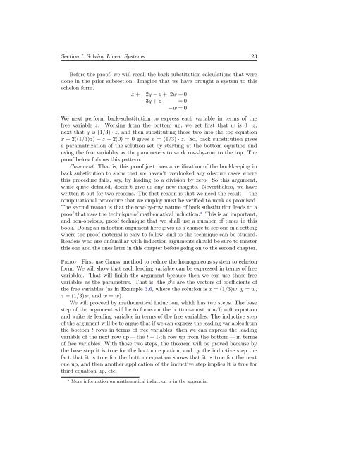
Section I. Solving Linear Systems 23Before the proof, we will recall the back substitution calculations that weredone in the prior subsection. Imagine that we have brought a system to thisechelon form.x + 2y − z + 2w = 0−3y + z = 0−w = 0We next perform back-substitution to express each variable in terms of thefree variable z. Working from the bottom up, we get first that w is 0 · z,next that y is (1/3) · z, and then substituting those two into the top equationx + 2((1/3)z) − z + 2(0) = 0 gives x = (1/3) · z. So, back substitution givesa paramatrization of the solution set by starting at the bottom equation andusing the free variables as the parameters to work row-by-row to the top. Theproof below follows this pattern.Comment: That is, this proof just does a verification of the bookkeeping inback substitution to show that we haven’t overlooked any obscure cases wherethis procedure fails, say, by leading to a division by zero. So this argument,while quite detailed, doesn’t give us any new insights. Nevertheless, we havewritten it out for two reasons. The first reason is that we need the result — thecomputational procedure that we employ must be verified to work as promised.The second reason is that the row-by-row nature of back substitution leads to aproof that uses the technique of mathematical induction. ∗ This is an important,and non-obvious, proof technique that we shall use a number of times in thisbook. Doing an induction argument here gives us a chance to see one in a settingwhere the proof material is easy to follow, and so the technique can be studied.Readers who are unfamiliar with induction arguments should be sure to masterthis one and the ones later in this chapter before going on to the second chapter.Proof. First use Gauss’ method to reduce the homogeneous system to echelonform. We will show that each leading variable can be expressed in terms of freevariables. That will finish the argument because then we can use those freevariables as the parameters. That is, the β’s ⃗ are the vectors of coefficients ofthe free variables (as in Example 3.6, where the solution is x = (1/3)w, y = w,z = (1/3)w, and w = w).We will proceed by mathematical induction, which has two steps. The basestep of the argument will be to focus on the bottom-most non-‘0 = 0’ equationand write its leading variable in terms of the free variables. The inductive stepof the argument will be to argue that if we can express the leading variables fromthe bottom t rows in terms of free variables, then we can express the leadingvariable of the next row up — the t + 1-th row up from the bottom — in termsof free variables. With those two steps, the theorem will be proved because bythe base step it is true for the bottom equation, and by the inductive step thefact that it is true for the bottom equation shows that it is true for the nextone up, and then another application of the inductive step implies it is true forthird equation up, etc.∗ More information on mathematical induction is in the appendix.