- Page 2:
Exact Solutions of Einstein’s Fie
- Page 7 and 8:
CAMBRIDGE UNIVERSITY PRESSCambridge
- Page 10 and 11:
Contentsix8 Continuous groups of tr
- Page 12 and 13:
Contentsxi15 Groups G 3 on non-null
- Page 14 and 15:
Contentsxiii21.1.4 Complexification
- Page 16 and 17:
Contentsxv29.2 Some general classes
- Page 18 and 19:
Contentsxvii34.1.3 Complex invarian
- Page 20 and 21:
PrefaceWhen, in 1975, two of the au
- Page 22:
Prefacexxifor tolerating our incess
- Page 25 and 26:
xxivList of Tables13.2 Subgroups G
- Page 28 and 29:
NotationAll symbols are explained i
- Page 30:
NotationxxixCurvature 2-forms: Θ a
- Page 33 and 34:
2 1 Introductionother fields and ma
- Page 35 and 36:
4 1 Introductionin physical applica
- Page 37 and 38:
6 1 Introductionfluids, scalar, Dir
- Page 39 and 40:
8 1 Introductionsince it is in prin
- Page 41 and 42:
10 2 Differential geometry without
- Page 43 and 44:
12 2 Differential geometry without
- Page 45 and 46:
14 2 Differential geometry without
- Page 47 and 48:
16 2 Differential geometry without
- Page 49 and 50:
18 2 Differential geometry without
- Page 51 and 52:
20 2 Differential geometry without
- Page 53 and 54:
22 2 Differential geometry without
- Page 55 and 56:
24 2 Differential geometry without
- Page 57 and 58:
26 2 Differential geometry without
- Page 59 and 60:
28 2 Differential geometry without
- Page 61 and 62:
3Some topics in Riemannian geometry
- Page 63 and 64:
32 3 Some topics in Riemannian geom
- Page 65 and 66:
The Outbreak of the Napoleonic Wars
- Page 67 and 68:
36 3 Some topics in Riemannian geom
- Page 69 and 70:
38 3 Some topics in Riemannian geom
- Page 71 and 72:
40 3 Some topics in Riemannian geom
- Page 73 and 74:
42 3 Some topics in Riemannian geom
- Page 75 and 76:
44 3 Some topics in Riemannian geom
- Page 77 and 78:
46 3 Some topics in Riemannian geom
- Page 79 and 80:
4The Petrov classificationThere are
- Page 81 and 82:
50 4 The Petrov classificationTable
- Page 83 and 84:
52 4 The Petrov classificationforms
- Page 85 and 86:
54 4 The Petrov classificationand s
- Page 87 and 88:
56 4 The Petrov classificationI✠I
- Page 89 and 90:
58 5 Classification of the Ricci te
- Page 91 and 92:
60 5 Classification of the Ricci te
- Page 93 and 94:
62 5 Classification of the Ricci te
- Page 95 and 96:
64 5 Classification of the Ricci te
- Page 97 and 98:
66 5 Classification of the Ricci te
- Page 99 and 100:
6Vector fields6.1 Vector fields and
- Page 101 and 102:
70 6 Vector fields6.1.1 Timelike un
- Page 103 and 104:
72 6 Vector fields6.2 Vector fields
- Page 105 and 106:
74 6 Vector fieldsTheorem 6.4 For s
- Page 107 and 108:
76 7 The Newman-Penrose and related
- Page 109 and 110:
78 7 The Newman-Penrose and related
- Page 111 and 112:
80 7 The Newman-Penrose and related
- Page 113 and 114:
82 7 The Newman-Penrose and related
- Page 115 and 116:
84 7 The Newman-Penrose and related
- Page 117 and 118:
86 7 The Newman-Penrose and related
- Page 119 and 120:
88 7 The Newman-Penrose and related
- Page 121 and 122:
90 7 The Newman-Penrose and related
- Page 123 and 124:
92 8 Continuous groups of transform
- Page 125 and 126:
94 8 Continuous groups of transform
- Page 127 and 128:
96 8 Continuous groups of transform
- Page 129 and 130:
98 8 Continuous groups of transform
- Page 131 and 132:
100 8 Continuous groups of transfor
- Page 133 and 134:
102 8 Continuous groups of transfor
- Page 135 and 136:
104 8 Continuous groups of transfor
- Page 137 and 138:
106 8 Continuous groups of transfor
- Page 139 and 140:
108 8 Continuous groups of transfor
- Page 141 and 142:
110 8 Continuous groups of transfor
- Page 143 and 144:
9Invariants and the characterizatio
- Page 145 and 146:
114 9 Invariants and the characteri
- Page 147 and 148:
116 9 Invariants and the characteri
- Page 149 and 150:
118 9 Invariants and the characteri
- Page 151 and 152:
120 9 Invariants and the characteri
- Page 153 and 154:
122 9 Invariants and the characteri
- Page 155 and 156:
124 9 Invariants and the characteri
- Page 157 and 158:
126 9 Invariants and the characteri
- Page 159 and 160:
128 9 Invariants and the characteri
- Page 161 and 162:
130 10 Generation techniquesarbitra
- Page 163 and 164:
132 10 Generation techniquesEinstei
- Page 166 and 167:
10.3 Symmetries more general than L
- Page 168 and 169:
10.4 Prolongation 137Other examples
- Page 170 and 171:
10.4 Prolongation 139If there were
- Page 172 and 173:
Stokes’s theorem we have10.4 Prol
- Page 174 and 175:
10.4 Prolongation 143The terms with
- Page 176 and 177:
10.5 Solutions of the linearized eq
- Page 178 and 179:
10.6 Bäcklund transformations 147T
- Page 180 and 181:
10.8 Harmonic maps 149with a Lagran
- Page 182 and 183:
10.9 Variational Bäcklund transfor
- Page 184 and 185:
10.11 Generation methods includingp
- Page 186 and 187:
10.11 Generation methods includingp
- Page 188 and 189:
Part IISolutions with groups of mot
- Page 190 and 191:
11.2 Isotropy and the curvature ten
- Page 192 and 193:
11.2 Isotropy and the curvature ten
- Page 194 and 195:
11.3 The possible space-times with
- Page 196 and 197:
Table 11.2. Solutions with proper h
- Page 198 and 199:
11.4 Summary of solutions with homo
- Page 200 and 201:
p − 1 )(y∂ y + z∂z) Table 11.
- Page 202 and 203:
12Homogeneous space-times12.1 The p
- Page 204 and 205:
12.1 The possible metrics 173deriva
- Page 206 and 207:
12.3 Homogeneous non-null electroma
- Page 208 and 209:
12.4 Homogeneous perfect fluid solu
- Page 210 and 211:
12.4 Homogeneous perfect fluid solu
- Page 212 and 213:
12.6 Summary 181Table 12.1.Homogene
- Page 214 and 215:
13Hypersurface-homogeneous space-ti
- Page 216 and 217:
13.1 The possible metrics 185The ex
- Page 218 and 219:
13.1 The possible metrics 187Summar
- Page 220 and 221:
13.2 Formulations of the field equa
- Page 222 and 223:
13.2 Formulations of the field equa
- Page 224 and 225:
13.2 Formulations of the field equa
- Page 226 and 227:
13.3 Vacuum, Λ-term and Einstein-M
- Page 228 and 229:
13.3 Vacuum, Λ-term and Einstein-M
- Page 230 and 231:
13.3 Vacuum, Λ-term and Einstein-M
- Page 232 and 233:
13.3 Vacuum, Λ-term and Einstein-M
- Page 234 and 235:
13.3 Vacuum, Λ-term and Einstein-M
- Page 236 and 237:
13.4 Perfect fluid solutions homoge
- Page 238 and 239:
13.5 Summary of all metrics with G
- Page 240 and 241:
Table 13.4. Solutions given explici
- Page 242:
14.2 Robertson-Walker cosmologies 2
- Page 245 and 246:
214 14 Spatially-homogeneous perfec
- Page 247 and 248:
216 14 Spatially-homogeneous perfec
- Page 249 and 250:
218 14 Spatially-homogeneous perfec
- Page 251 and 252:
220 14 Spatially-homogeneous perfec
- Page 253 and 254:
222 14 Spatially-homogeneous perfec
- Page 255 and 256:
224 14 Spatially-homogeneous perfec
- Page 257 and 258:
15Groups G 3 on non-null orbits V 2
- Page 259 and 260:
228 15 Groups G 3 on non-null orbit
- Page 261 and 262:
230 15 Groups G 3 on non-null orbit
- Page 263 and 264:
232 15 Groups G 3 on non-null orbit
- Page 265 and 266:
234 15 Groups G 3 on non-null orbit
- Page 267 and 268: 236 15 Groups G 3 on non-null orbit
- Page 269 and 270: 238 15 Groups G 3 on non-null orbit
- Page 271 and 272: 240 15 Groups G 3 on non-null orbit
- Page 273 and 274: 242 15 Groups G 3 on non-null orbit
- Page 275 and 276: 244 15 Groups G 3 on non-null orbit
- Page 277 and 278: 246 15 Groups G 3 on non-null orbit
- Page 279 and 280: 248 16 Spherically-symmetric perfec
- Page 281 and 282: 250 16 Spherically-symmetric perfec
- Page 283 and 284: 252 16 Spherically-symmetric perfec
- Page 285 and 286: 254 16 Spherically-symmetric perfec
- Page 287 and 288: 256 16 Spherically-symmetric perfec
- Page 289 and 290: 258 16 Spherically-symmetric perfec
- Page 291 and 292: 260 16 Spherically-symmetric perfec
- Page 293 and 294: 262 16 Spherically-symmetric perfec
- Page 295 and 296: 17Groups G 2 and G 1 on non-null or
- Page 297 and 298: 266 17 Groups G 2 and G 1 on non-nu
- Page 299 and 300: 268 17 Groups G 2 and G 1 on non-nu
- Page 301 and 302: 270 17 Groups G 2 and G 1 on non-nu
- Page 303 and 304: 272 17 Groups G 2 and G 1 on non-nu
- Page 305 and 306: 274 17 Groups G 2 and G 1 on non-nu
- Page 307 and 308: 276 18 Stationary gravitational fie
- Page 309 and 310: 278 18 Stationary gravitational fie
- Page 311 and 312: 280 18 Stationary gravitational fie
- Page 313 and 314: 282 18 Stationary gravitational fie
- Page 315 and 316: 284 18 Stationary gravitational fie
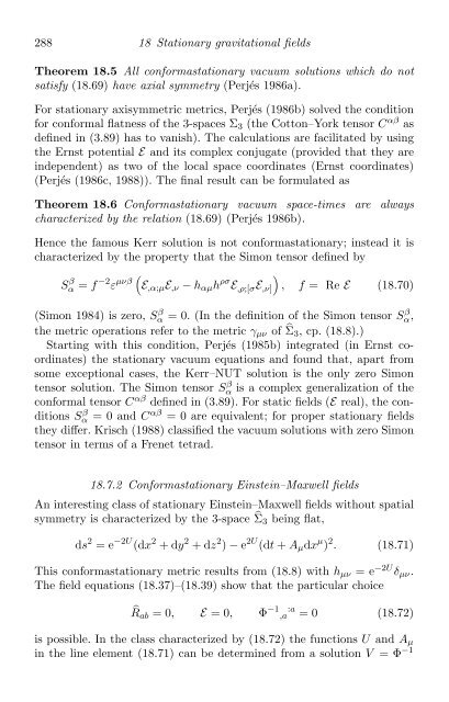
- Page 317: 286 18 Stationary gravitational fie
- Page 321 and 322: 290 18 Stationary gravitational fie
- Page 323 and 324: 19Stationary axisymmetric fields: b
- Page 325 and 326: 294 19 Stationary axisymmetric fiel
- Page 327 and 328: 296 19 Stationary axisymmetric fiel
- Page 329 and 330: 298 19 Stationary axisymmetric fiel
- Page 331 and 332: 300 19 Stationary axisymmetric fiel
- Page 333 and 334: 302 19 Stationary axisymmetric fiel
- Page 335 and 336: 20Stationary axisymmetric vacuumsol
- Page 337 and 338: 306 20 Stationary axisymmetric vacu
- Page 339 and 340: 308 20 Stationary axisymmetric vacu
- Page 341 and 342: 310 20 Stationary axisymmetric vacu
- Page 343 and 344: 312 20 Stationary axisymmetric vacu
- Page 345 and 346: 314 20 Stationary axisymmetric vacu
- Page 347 and 348: 316 20 Stationary axisymmetric vacu
- Page 349 and 350: 318 20 Stationary axisymmetric vacu
- Page 351 and 352: 320 21 Non-empty stationary axisymm
- Page 353 and 354: 322 21 Non-empty stationary axisymm
- Page 355 and 356: 324 21 Non-empty stationary axisymm
- Page 357 and 358: 326 21 Non-empty stationary axisymm
- Page 359 and 360: 328 21 Non-empty stationary axisymm
- Page 361 and 362: 330 21 Non-empty stationary axisymm
- Page 363 and 364: 332 21 Non-empty stationary axisymm
- Page 365 and 366: 334 21 Non-empty stationary axisymm
- Page 367 and 368: 336 21 Non-empty stationary axisymm
- Page 369 and 370:
338 21 Non-empty stationary axisymm
- Page 371 and 372:
340 21 Non-empty stationary axisymm
- Page 373 and 374:
342 22 Groups G 2 I on spacelike or
- Page 375 and 376:
344 22 Groups G 2 I on spacelike or
- Page 377 and 378:
346 22 Groups G 2 I on spacelike or
- Page 379 and 380:
348 22 Groups G 2 I on spacelike or
- Page 381 and 382:
350 22 Groups G 2 I on spacelike or
- Page 383 and 384:
352 22 Groups G 2 I on spacelike or
- Page 385 and 386:
354 22 Groups G 2 I on spacelike or
- Page 387 and 388:
356 22 Groups G 2 I on spacelike or
- Page 389 and 390:
23Inhomogeneous perfect fluid solut
- Page 391 and 392:
360 23 Inhomogeneous perfect fluid
- Page 393 and 394:
362 23 Inhomogeneous perfect fluid
- Page 395 and 396:
364 23 Inhomogeneous perfect fluid
- Page 397 and 398:
366 23 Inhomogeneous perfect fluid
- Page 399 and 400:
368 23 Inhomogeneous perfect fluid
- Page 401 and 402:
370 23 Inhomogeneous perfect fluid
- Page 403 and 404:
372 23 Inhomogeneous perfect fluid
- Page 405 and 406:
374 23 Inhomogeneous perfect fluid
- Page 407 and 408:
376 24 Groups on null orbits. Plane
- Page 409 and 410:
378 24 Groups on null orbits. Plane
- Page 411 and 412:
380 24 Groups on null orbits. Plane
- Page 413 and 414:
382 24 Groups on null orbits. Plane
- Page 415 and 416:
384 24 Groups on null orbits. Plane
- Page 417 and 418:
386 24 Groups on null orbits. Plane
- Page 419 and 420:
388 25 Collision of plane wavesIVII
- Page 421 and 422:
390 25 Collision of plane waveswhic
- Page 423 and 424:
392 25 Collision of plane wavesone
- Page 425 and 426:
394 25 Collision of plane wavesErez
- Page 427 and 428:
396 25 Collision of plane wavesfron
- Page 429 and 430:
398 25 Collision of plane waves2V u
- Page 431 and 432:
400 25 Collision of plane wavesThe
- Page 433 and 434:
402 25 Collision of plane waves(a,
- Page 435 and 436:
404 25 Collision of plane wavesAssu
- Page 437 and 438:
406 25 Collision of plane wavessolu
- Page 439 and 440:
408 26 The various classes of algeb
- Page 441 and 442:
410 26 The various classes of algeb
- Page 443 and 444:
412 26 The various classes of algeb
- Page 445 and 446:
414 26 The various classes of algeb
- Page 447 and 448:
27The line element for metrics with
- Page 449 and 450:
418 27 The line element for κ = σ
- Page 451 and 452:
420 27 The line element for κ = σ
- Page 453 and 454:
28Robinson-Trautman solutions28.1 R
- Page 455 and 456:
424 28 Robinson-Trautman solutionsT
- Page 457 and 458:
426 28 Robinson-Trautman solutionsr
- Page 459 and 460:
428 28 Robinson-Trautman solutionsW
- Page 461 and 462:
430 28 Robinson-Trautman solutionsf
- Page 463 and 464:
432 28 Robinson-Trautman solutionsE
- Page 465 and 466:
434 28 Robinson-Trautman solutionsh
- Page 467 and 468:
436 28 Robinson-Trautman solutionsw
- Page 469 and 470:
438 29 Twistingvacuum solutionsthen
- Page 471 and 472:
440 29 Twistingvacuum solutions29.1
- Page 473 and 474:
442 29 Twistingvacuum solutionsThe
- Page 475 and 476:
444 29 Twistingvacuum solutionsTabl
- Page 477 and 478:
446 29 Twistingvacuum solutions29.2
- Page 479 and 480:
448 29 Twistingvacuum solutionsThe
- Page 481 and 482:
450 29 Twistingvacuum solutionsFor
- Page 483 and 484:
452 29 Twistingvacuum solutionsThe
- Page 485 and 486:
454 29 Twistingvacuum solutionscove
- Page 487 and 488:
456 30 TwistingEinstein-Maxwell and
- Page 489 and 490:
458 30 TwistingEinstein-Maxwell and
- Page 491 and 492:
460 30 TwistingEinstein-Maxwell and
- Page 493 and 494:
462 30 TwistingEinstein-Maxwell and
- Page 495 and 496:
464 30 TwistingEinstein-Maxwell and
- Page 497 and 498:
466 30 TwistingEinstein-Maxwell and
- Page 499 and 500:
468 30 TwistingEinstein-Maxwell and
- Page 501 and 502:
31Non-diverging solutions (Kundt’
- Page 503 and 504:
472 31 Non-diverging solutions (Kun
- Page 505 and 506:
474 31 Non-diverging solutions (Kun
- Page 507 and 508:
476 31 Non-diverging solutions (Kun
- Page 509 and 510:
478 31 Non-diverging solutions (Kun
- Page 511 and 512:
480 31 Non-diverging solutions (Kun
- Page 513 and 514:
482 31 Non-diverging solutions (Kun
- Page 515 and 516:
484 31 Non-diverging solutions (Kun
- Page 517 and 518:
486 32 Kerr-Schild metricsThese rel
- Page 519 and 520:
488 32 Kerr-Schild metricsay ( u )
- Page 521 and 522:
490 32 Kerr-Schild metricsTheorem 3
- Page 523 and 524:
492 32 Kerr-Schild metricsTable 32.
- Page 525 and 526:
494 32 Kerr-Schild metricsHence k i
- Page 527 and 528:
496 32 Kerr-Schild metricsThe only
- Page 529 and 530:
498 32 Kerr-Schild metricssticking
- Page 531 and 532:
500 32 Kerr-Schild metricswhere bot
- Page 533 and 534:
502 32 Kerr-Schild metricsIf we now
- Page 535 and 536:
504 32 Kerr-Schild metrics(Martín
- Page 537 and 538:
33Algebraically special perfect flu
- Page 539 and 540:
508 33 Algebraically special perfec
- Page 541 and 542:
510 33 Algebraically special perfec
- Page 543 and 544:
512 33 Algebraically special perfec
- Page 545 and 546:
514 33 Algebraically special perfec
- Page 547 and 548:
516 33 Algebraically special perfec
- Page 549 and 550:
Part IVSpecial methods34Application
- Page 551 and 552:
520 34 Application of generation te
- Page 553 and 554:
522 34 Application of generation te
- Page 555 and 556:
524 34 Application of generation te
- Page 557 and 558:
526 34 Application of generation te
- Page 559 and 560:
528 34 Application of generation te
- Page 561 and 562:
530 34 Application of generation te
- Page 563 and 564:
532 34 Application of generation te
- Page 565 and 566:
534 34 Application of generation te
- Page 567 and 568:
536 34 Application of generation te
- Page 569 and 570:
538 34 Application of generation te
- Page 571 and 572:
540 34 Application of generation te
- Page 573 and 574:
542 34 Application of generation te
- Page 575 and 576:
544 34 Application of generation te
- Page 577 and 578:
546 34 Application of generation te
- Page 579 and 580:
548 34 Application of generation te
- Page 581 and 582:
550 34 Application of generation te
- Page 583 and 584:
552 34 Application of generation te
- Page 585 and 586:
554 35 Special vector and tensor fi
- Page 587 and 588:
556 35 Special vector and tensor fi
- Page 589 and 590:
558 35 Special vector and tensor fi
- Page 591 and 592:
560 35 Special vector and tensor fi
- Page 593 and 594:
562 35 Special vector and tensor fi
- Page 595 and 596:
564 35 Special vector and tensor fi
- Page 597 and 598:
566 35 Special vector and tensor fi
- Page 599 and 600:
568 35 Special vector and tensor fi
- Page 601 and 602:
570 35 Special vector and tensor fi
- Page 603 and 604:
572 36 Solutions with special subsp
- Page 605 and 606:
574 36 Solutions with special subsp
- Page 607 and 608:
576 36 Solutions with special subsp
- Page 609 and 610:
578 36 Solutions with special subsp
- Page 611 and 612:
37Local isometric embedding offour-
- Page 613 and 614:
582 37 Embeddingof four-dimensional
- Page 615 and 616:
584 37 Embeddingof four-dimensional
- Page 617 and 618:
586 37 Embeddingof four-dimensional
- Page 619 and 620:
588 37 Embeddingof four-dimensional
- Page 621 and 622:
590 37 Embeddingof four-dimensional
- Page 623 and 624:
592 37 Embeddingof four-dimensional
- Page 625 and 626:
594 37 Embeddingof four-dimensional
- Page 627 and 628:
596 37 Embeddingof four-dimensional
- Page 629 and 630:
598 37 Embeddingof four-dimensional
- Page 631 and 632:
600 37 Embeddingof four-dimensional
- Page 633 and 634:
602 37 Embeddingof four-dimensional
- Page 635 and 636:
604 37 Embeddingof four-dimensional
- Page 637 and 638:
606 38 The interconnections between
- Page 639 and 640:
608 38 The interconnections between
- Page 641 and 642:
610 38 The interconnections between
- Page 643 and 644:
612 38 The interconnections between
- Page 645 and 646:
Table 38.10. Algebraically special
- Page 647 and 648:
616 ReferencesAlencar, P.S.C. and L
- Page 649 and 650:
618 ReferencesBasu, A., Ganguly, S.
- Page 651 and 652:
620 ReferencesBirkhoff, G.D. (1923)
- Page 653 and 654:
622 ReferencesBradley, M.and Karlhe
- Page 655 and 656:
624 ReferencesCarminati, J.(1981).A
- Page 657 and 658:
626 ReferencesCharach, Ch.and Malin
- Page 659 and 660:
628 ReferencesCollinson, C.D. (1964
- Page 661 and 662:
630 ReferencesDas, K.C. and Chaudhu
- Page 663 and 664:
632 ReferencesDemiański, M.and New
- Page 665 and 666:
634 ReferencesEhlers, J.(1961).Beit
- Page 667 and 668:
636 ReferencesFernandez-Jambrina, L
- Page 669 and 670:
638 ReferencesGarcía D., A. and Br
- Page 671 and 672:
640 ReferencesGowdy, R.H. (1975). C
- Page 673 and 674:
642 ReferencesHajj-Boutros, J.(1985
- Page 675 and 676:
644 ReferencesHarrison, B.K. (1978)
- Page 677 and 678:
646 ReferencesHerlt, E.(1972).Über
- Page 679 and 680:
648 ReferencesHoenselaers, C.(1992)
- Page 681 and 682:
650 ReferencesIvanov, B.Y. (1999).
- Page 683 and 684:
652 ReferencesKerns, R.M. and Wild,
- Page 685 and 686:
654 ReferencesKolassis, C.and Griff
- Page 687 and 688:
656 ReferencesKramer, D.and Neugeba
- Page 689 and 690:
658 ReferencesKyriakopoulos, E.(198
- Page 691 and 692:
660 ReferencesLi, W.and Ernst, F.J.
- Page 693 and 694:
662 ReferencesLun, A.W.C., McIntosh
- Page 695 and 696:
664 ReferencesMarder, L.(1969).Grav
- Page 697 and 698:
666 ReferencesMehra, A.L. (1966). R
- Page 699 and 700:
668 ReferencesNeugebauer, G.and Mei
- Page 701 and 702:
670 ReferencesPant, D.N. (1994). Va
- Page 703 and 704:
672 ReferencesPiper, M.S.(1997).Com
- Page 705 and 706:
674 ReferencesRobertson, H.P. (1929
- Page 707 and 708:
676 ReferencesSchmidt, B.G. (1996).
- Page 709 and 710:
678 ReferencesSingleton, D.B. (1990
- Page 711 and 712:
680 ReferencesStewart, B.W., Witten
- Page 713 and 714:
682 ReferencesTeixeira, A.F.F., Wol
- Page 715 and 716:
684 ReferencesVaidya, P.C. and Pate
- Page 717 and 718:
686 References65th birthday, ed. M.
- Page 719 and 720:
688 ReferencesXanthopoulos, B.C. (1
- Page 721 and 722:
Indexacceleration, 70affine colline
- Page 723 and 724:
692 Indexdust solutionsFriedmann un
- Page 725 and 726:
694 IndexHarrison solutions, 272Har
- Page 727 and 728:
696 IndexNUT solution, 310, 449, 45
- Page 729 and 730:
698 IndexRiemann tensor, 25, 34cova
- Page 731 and 732:
700 Indextype D solutions (contd)Ro