Online proceedings - EDA Publishing Association
Online proceedings - EDA Publishing Association
Online proceedings - EDA Publishing Association
- No tags were found...

Create successful ePaper yourself
Turn your PDF publications into a flip-book with our unique Google optimized e-Paper software.
http://cmp.imag.fr/conferences/therminic2008/The Workshop is sponsored by the IEEE Components, Packaging,and Manufacturing Technology Society and by CMP.CNRS - INPG - UJF
COLLECTION OF PAPERS PRESENTED AT THE14 th International Workshop onTHERMal INvestigation of ICsand SystemsRome, Italy24 - 26 September 2008Sponsored by:The Institute of Electrical & ElectronicsEngineers, Inc.IEEE Components, Packaging andManufacturing Technology Society
24-26 September 2008, Rome, Italy©<strong>EDA</strong> <strong>Publishing</strong> <strong>Association</strong> /THERMINIC2008 ISBN: 978-2-35500-008-9© Color cover design by STIM IEEE Catalog Number: CFP08TII-PRTAbstracting / Indexing:• Cambridge Scientific Abstracts• INSPEC• PASCAL• CEDOCAR• British Library’s OPAC• TIB• BNF• SUDOCRepositories:• IEEE XPLORE• CNRS/HAL Open Archives• ArXiv Open Archives• EU Funded Driver Project Open ArchivesAdditional copies of this PROCEEDINGS or copies of previous years may be purchased from:CMP, 46 Avenue Félix Viallet, 38031 Grenoble, France.Fax: +33 4 76 47 38 14 –Order forms available at: http://cmp.imag.fr/conferences Visit <strong>EDA</strong> <strong>Publishing</strong> <strong>Association</strong> http://www.eda-publishing.org Since 2005 <strong>proceedings</strong> are available on-line.©<strong>EDA</strong> <strong>Publishing</strong>/THERMINIC 2008 IIISBN: 978-2-35500-008-9
24-26 September 2008, Rome, ItalyWORKSHOP COMMITTEE:General Chair:Vice General Chair:Programme Chairs:Bernard Courtois, CMP, Grenoble, FranceMárta Rencz, Budapest Univ. of Technology and Economics (BUTE), HungaryClemens Lasance, Philips Eindhoven, The NetherlandsVladimir Székely, Budapest Univ. of Technology and Economics (BUTE), HungaryPROGRAMME COMMITTEE:Attila Aranyosi, Electronic Cooling Solutions Inc.Tetsuya Baba, Nat. Metrology Institute Tsukuba, JapanTine Baelmans, KUL, BelgiumIstvan Barsony, KFKI-ATKI, HungaryDavid Blackburn, NIST, USAKrish Chakrabarty, Duke, USABenoit Charlot, IES, Montpellier, FranceHerming Chiueh, National Chiao Tung U., TaiwanFilip Christiaens, Alcatel Bell, BelgiumWilfrid Claeys, U. Bordeaux, FranceLorenzo Codecasa, Polit. di Milano, ItalyAbishai Daniel, Intel, USAGilbert De Mey, Ghent U., BelgiumRyusuke Egawa, Tohoku U., JapanWaleed Faris, IIUM, MalaysiaSuresh Garimella, Purdue U., West Lafayette, USAYork Christian Gerstenmaier, Siemens, GermanyYogesh Gianchandani, U. of Michigan, USAAri Glezer, The Georgia Inst. of Techno., USABruce Guenin, Sun Microsystems, USAJohn Janssen, NXP Semiconductors, Nijmegen, The NetherlandsBruno Michel, IBM Zurich, Rueschlikon, SwitzerlandTadao Nakamura, U. of Tohoku, JapanAndrzej Napieralski, TU Lodz, PolandVenkat Natarajan, Intel India Pvt. Ltd., Bangalore, IndiaHeinz Pape, Infineon Techn., GermanyAnne-Claire Pliska, CSEM, Neuchâtel, SwitzerlandAndrás Poppe, BUTE, Budapest, HungaryPeter Raad, South. Methodist U., USAPeter Rodgers, The Petroleum Inst., UAEAntonio Rubio, UPC, SpainMohamed-Nabil Sabry, U. Française d’Égypte, EgyptYves Scudeller, E.Polytech. U. Nantes, FranceAli Shakouri, U. of California, USAMoowhan Shin, Myong Ji U., KoreaEphraim Suhir, U.C Santa Cruz, USAAndrew Tay, NUS, SingaporeBart Vandevelde, IMEC, BelgiumGerhard Wachutka, TU München, GermanyKazuaki Yazawa, Sony, Tokyo, JapanThomas Zahner, OSRAM, GermanyAttila Aranyosi, Electronic Cooling Solutions Inc.Joan Yu, Philips Lumileds Lighting Company, Netherlands©<strong>EDA</strong> <strong>Publishing</strong>/THERMINIC 2008 IIIISBN: 978-2-35500-008-9
24-26 September 2008, Rome, Italy©<strong>EDA</strong> <strong>Publishing</strong>/THERMINIC 2008 ISBN: 978-2-35500-008-9IV
24-26 September 2008, Rome, ItalyPREFACETHERMINIC Workshops are a series of events to discuss the essential thermal questions of microelectronicmicrostructures and electronic parts in general. These questions are becoming more and more crucial with the increasingelement density of circuits packaged together and with the move to nanotechnology. Thermal management is expected tobecome an increasingly dominating factor of the cost of the total system. All these trends are calling for thermalsimulation, monitoring and cooling. New developments such as the moving parts of microsystems raise new thermalproblems to be solved in the near future necessitating the regular discussion of the experts in these fields. In addition,new materials have to be created to assure the manageability of the increased thermal stress and to answer the challengesof the nano-era.Previous THERMINIC Workshops have been held in Grenoble (1995), Budapest (1996), Cannes (1997 and 1998), Rome(1999), Budapest (2000), Paris (2001) Madrid (2002), Aix-en-Provence (2003) Sophia Antipolis (2004), Belgirate (2005)in Nice (2006) and Budapest (2007).The programme of 2008 includes 2 invited talks, 2 panels, 1 embedded tutorial, 28 oral in 7 sessions and 16 posterpresentations.Out of the submissions accepted by the Programme Committee, this volume -- which is the informal <strong>proceedings</strong> of theWorkshop -- contains the paper versions of one invited speaker presentation, the embedded tutorial presentations, 25 oralpresentations and 16 poster presentations.We would like to express our sincere appreciation to the authors for their high quality contributions, their cooperationand efforts. In addition, we would like to thank the members of the Workshop Programme Committee for carrying outthe paper selection work with care and competence.Bernard CourtoisGeneral ChairVladimir SzékelyProgramme ChairMárta RenczVice General ChairClemens LasanceProgramme Chair©<strong>EDA</strong> <strong>Publishing</strong>/THERMINIC 2008 VISBN: 978-2-35500-008-9
24-26 September 2008, Rome, Italy©<strong>EDA</strong> <strong>Publishing</strong>/THERMINIC 2008 VIISBN: 978-2-35500-008-9
24-26 September 2008, Rome, ItalyTable of ContentsWednesday, September 24 th , 2008Invited speaker 1: CFD for Electronics Cooling: MCAD and <strong>EDA</strong> Embedded vs. StandaloneCFD FOR ELECTRONICS COOLING: MCAD AND <strong>EDA</strong> EMBEDDED vs. STAND-ALONE . . . . . . . . . . . . . . . . . 1John Parry, Flomerics, Hampton Court, UKSession 1: MeasurementsTRIANGULATION METHOD FOR STRUCTURE FUNCTIONS OF MULTI-DIRECTIONAL HEAT-FLOWS . . 8Lorenzo Codecasa, Dario D’Amore and Paolo Maffezzoni, Politecnico di Milano, ItalyTRANSIENT DUAL INTERFACE MEASUREMENT OF THE RTH-JC OF POWER PACKAGES . . . . . . . . . . . . . 14Dirk Schweitzer, Infineon Technologies AG, GermanyEVALUATION OF SHORT PULSE THERMAL TRANSIENT MEASUREMENTS . . . . . . . . . . . . . . . . . . . . . . . . . . . 20Vladimir Szekely, Budapest University of Technology & Economics, HungaryNEW APPROACH FOR THERMAL INVESTIGATION OF A III-V POWER TRANSISTOR . . . . . . . . . . . . . . . . . . 26Maxime Fontaine, Eric Joubert, Olivier Latry, Pascal Dherbecourt and Mohamed Ketata, LEMI, FranceSession 2: Reliability issuesENSURING TEMPERATURE-INSENSITIVITY OF DUAL-VT DESIGNS THROUGH ITD-AWARESYNTHESIS . . . . . . . . . . . . . . . . . . . . . . . . . . . . . . . . . . . . . . . . . . . . . . . . . . . . . . . . . . . . . . . . . . . . . . . . . . . . . . . . . . . . . . . . . . . . 31Andrea Calimera, Politecnico di Torino, Italy; Ruth Iris Bahar, Brown University, USA; Enrico Macii and MassimoPoncino, Politecnico di Torino, ItalyMANAGING LEAKAGE POWER AND RELIABILITY IN HOT CHIPS USING SYSTEM FLOORPLANNINGAND SRAM DESIGN . . . . . . . . . . . . . . . . . . . . . . . . . . . . . . . . . . . . . . . . . . . . . . . . . . . . . . . . . . . . . . . . . . . . . . . . . . . . . . . . . . . 37Aseem Gupta, Amin Djahromi, Ahmed Eltawil, Fadi Kurdahi, Nikil Dutt, University of California Irvine, USA;Kamal Khouri and Magdy Abadir, Freescale Semiconductor Inc., USAASSESMENT OF DIE ATTACH QUALITY BY ANALYSIS OF CIRCUIT THERMAL RESPONSE SPECTRUM 43Marcin Janicki, Technical University of Lodz, Poland; Bjorn Vermeersch, Jedrzej Banaszczyk, University of Ghent,Belgium; Marek Kaminski, Technical University of Lodz, Poland; Gilbert De Mey, University of Ghent, Belgium;and Andrzej Napieralski, Technical Univarsity of Lodz, PolandMATERIAL CHARACTERISATION AND NON-DESTRUCTIVE FAILURE ANALYSIS BY TRANSIENTPULSE GENERATION AND IR-THERMOGRAPHY . . . . . . . . . . . . . . . . . . . . . . . . . . . . . . . . . . . . . . . . . . . . . . . . . . . . . . 47Daniel May, Bernhard Wunderle, Mohamad Abo Ras, Wolfgang Faust, Fraunhofer IZM, Germany; Astrid Gollhardt,AMIC GmbH, Germany; Heike Kukuk-Schmid and Bernd Michel, Fraunhofer IZM, GermanySession 3: Simulation at package levelCOMPACT THERMAL NETWORKS FOR CONJUGATE HEAT TRANSFER BY DIRECTIONAL MOMENTMATCHING . . . . . . . . . . . . . . . . . . . . . . . . . . . . . . . . . . . . . . . . . . . . . . . . . . . . . . . . . . . . . . . . . . . . . . . . . . . . . . . . . . . . . . . . . . . . 52Lorenzo Codecasa, Dario D’Amore and Paolo Maffezzoni, Politecnico di Milano, Italy©<strong>EDA</strong> <strong>Publishing</strong>/THERMINIC 2008 VIIISBN: 978-2-35500-008-9
24-26 September 2008, Rome, ItalyBLOCK-LEVEL THERMAL MODEL FOR FLOORPLAN STAGE IN VLSI DESIGN FLOW . . . . . . . . . . . . . . . . . 58Shun-Hua Lin, National Chiao Tung University, Taiwan; Jin-Tai Yan, Chung-Hua University, Taiwan; and HermingChiueh, National Chiao Tung University, TaiwanMULTISCALE 3D THERMAL ANALYSIS OF ANALOG ICS: FROM FULL-CHIP TO DEVICE LEVEL . . . . . . 64Marek Turowski, CFD Research Corporation (CFDRC), USA; Steven Dooley, Air Force Research Laboratory(AFRL), USA; Ashok Raman, CFD Research Corporation (CFDRC), USA; and Matthew Casto, Air Force ResearchLaboratory (AFRL), USATHE MINIMAL SET OF PARAMETERS FOR EXACT DYNAMIC THERMAL MODELS . . . . . . . . . . . . . . . . . . . . 70York Christian Gerstenmaier, Siemens AG, Germany; and Gerhard Wachutka, Munich University of Technology,GermanyPoster introduction and viewingAUTOMATIC ELECTRO-THERMAL ANALYSIS IN MENTOR GRAPHICS PCB DESIGN SYSTEM . . . . . . . . . 76Konstantin Petrosjanc and Petr Kozynko, MIEM, Russian FederationINTEGRATED THERMAL MODELING OF HETEROGENEOUS ECUBES STACKED DEVICES . . . . . . . . . . . . 80Grzegorz Janczyk, Tomasz Bieniek, Piotr Grabiec and Jerzy Szynka, Institute of Electron Technology, PolandLOGICAL EFFORT MODEL EXTENSION WITH TEMPERATURE AND VOLTAGE VARIATIONS . . . . . . . . . . 85Chun-Hui Wu, Shun-Hua Lin and Herming Chiueh, National Chiao Tung University, TaiwanA NOVEL PROCEDURE AND DEVICE TO ALLOW COMPREHENSIVE CHARACTERIZATION OF POWERLEDS OVER A WIDE RANGE OF TEMPERATURE. . . . . . . . . . . . . . . . . . . . . . . . . . . . . . . . . . . . . . . . . . . . . . . . . . . . . . . 89Gábor Molnár, Microelectronics Research and Development Ltd, Hungary; Gergely Nagy and Zoltán Szucs, BUTE,HungaryMULTI-PHYSICS ANALYSIS OF A PHOTOVOLTAIC PANEL WITH A HEAT RECOVERY SYSTEM . . . . . . . . 93Paolo Maffezzoni, Lorenzo Codecasa and Dario D’Amore, Politecnico di Milano, ItalyPHASE CHANGE HEAT DISSIPATER OF ALUMINIUM CONTAINER. . . . . . . . . . . . . . . . . . . . . . . . . . . . . . . . . . . . . 97Cecilia Wolluschek, E. Armendáriz and Jesús Esarte, Fundación CETENA, Noain, SpainTHERMAL DESIGN OF FULLY-ISOLATED BIPOLAR TRANSISTORS . . . . . . . . . . . . . . . . . . . . . . . . . . . . . . . . . . . . 101Salvatore Russo, Delft University of Technology / University of Naples Federico II, Netherlands; Luigi La Spina,Delft University of Technology, Netherlands; Vincenzo D’Alessandro, Niccolò Rinaldi, University of Naples FedericoII, Italy; and Lis K. Nanver, Delft University of Technology, NetherlandsTHERMAL TRANSIENT CHARACTERISATION OF COMPLEX CIRCUITS . . . . . . . . . . . . . . . . . . . . . . . . . . . . . . . 106Gergely Perlaky, Budapest Univ. of Technology, Hungary; and Gábor Farkas, MicReD Ltd., Budapest, HungaryIN-SITU MEASUREMENT OF VARIOUS THIN BOND-LINE-THICKNESS THERMAL INTERFACEMATERIALS WITH CORRELATION TO STRUCTURAL FEATURES . . . . . . . . . . . . . . . . . . . . . . . . . . . . . . . . . . . . . . 112Bernhard Wunderle, Jessica Kleff, Fraunhofer IZM, Germany; Raul Mrossko, AMIC, Germany; Daniel May, MohamadAbo Ras, Fraunhofer IZM, Germany; Ralph Schacht, FH Lausitz, Germany; Juergen Keller, Nanotest, Germany;Hermann Oppermann and Bernd Michel, Fraunhofer IZM, GermanyCOMPACT THERMAL MODELING OF ELECTRIC DOUBLE-LAYER CAPACITORS . . . . . . . . . . . . . . . . . . . . . . 118Philippe Guillemet, Caroline Pascot and Yves Scudeller, Université de Nantes, FranceHOT-CARRIER EFFECTS ON POWER RF LDMOS DEVICE RELIABILITY . . . . . . . . . . . . . . . . . . . . . . . . . . . . . . . 123Mohamed Ali Belaid and Kaouther Daoud-Ketata, GPM-UMR CNRS 6634, France©<strong>EDA</strong> <strong>Publishing</strong>/THERMINIC 2008 VIIIISBN: 978-2-35500-008-9
24-26 September 2008, Rome, ItalyTHERMAL CHARACTERIZATION AND MODELLING OF LITHIUM-BASED BATTERIES AT LOWTEMPERATURE AMBIENT . . . . . . . . . . . . . . . . . . . . . . . . . . . . . . . . . . . . . . . . . . . . . . . . . . . . . . . . . . . . . . . . . . . . . . . . . . . . . 128Domonkos Szente-Varga, Gyula Horváth and Marta Rencz, BUTE, HungaryDESIGN OF A STATIC TIM TESTER. . . . . . . . . . . . . . . . . . . . . . . . . . . . . . . . . . . . . . . . . . . . . . . . . . . . . . . . . . . . . . . . . . . . . 132Vladimir Szekely, Gergely Somlay, Péter G. Szabó and Marta Rencz, Budapest University of Technology & Economics,HungaryMULTITHREADING AND STRASSEN’S ALGORITHMS IN SUNRED FIELD SOLVER . . . . . . . . . . . . . . . . . . . . 137László Pohl, Budapest University of Technology and Economics, HungaryTHE SEMICONDUCTOR - DIELECTRIC INTERFACE FROM PN JUNCTION PERIPHERY AND ITSINFLUENCE ON RELIABILITY OF POWER DEVICES AT HIGH TEMPERATURE. . . . . . . . . . . . . . . . . . . . . . . . . 142Vasile Obreja, National R&D Institute for Microtechnology (IMT Bucuresti), RomaniaFPGA POWER MODEL FOR MINIMIZING THE THERMAL DISSIPATION . . . . . . . . . . . . . . . . . . . . . . . . . . . . . . . . 148bel Vámos and Marta Rencz, BUTE, HungaryThursday, September 25 th , 2008Invited speaker 2: Thermal conductivity in nanostructures: the role of acoustic phononsTHERMAL CONDUCTIVITY IN NANOSTRUCTURES: THE ROLE OF ACOUSTIC PHONONS . . . . . . . . . . . . 152Clivia. M. Sotomayor Torres, M. Schmidt, Catalan Institute of Nanotechnology, Spain; M. Prunnila and J. Ahopelto,VTT Micro and Nanoelectronics, FinlandSession 4: NanopackNANOPACK NANO PACKAGING TECHNOLOGY FOR INTERCONNECT AND HEAT DISSIPATION . . . . . . 153Afshin Ziaei and Sebastien Demoustier, Thales Research & Technology, FranceRECENT PROGRESS OF THERMAL INTERFACE MATERIAL RESEARCH - AN OVERVIEW. . . . . . . . . . . . . . 156Johan Liu, Chalmers University of Technology, SwedenBAND GAPS IN A PHONONIC CRYSTAL MADE OF A PERIODICAL ARRAY OF DOTS ON A PLATE . . . . . 163Bahram Djafari Rouhani and Yan Pennec, Institut d’Electronique, de Microélectronique et Nanotechnologies,FranceNANOSCALE MANAGEMENT OF ELECTRON-PHONON ENERGY TRANSFER . . . . . . . . . . . . . . . . . . . . . . . . . . 168Vladimir Mitin and Andrei Sergeev, SUNY at Buffalo, USASession 5: Novel and advanced coolingSILICON INTEGRATED VAPOR CHAMBER EQUIPPED WITH INTEGRATED SENSOR NETWORK FORIN-SITU THERMAL MONITORING AND COOLING OPTIMIZATION . . . . . . . . . . . . . . . . . . . . . . . . . . . . . . . . . . . . 173Bogdan Bercu, Laurent Montès and Panagiota Morfouli, IMEP, FranceMICRO CHANNEL HEATSINK OPTIMIZATION . . . . . . . . . . . . . . . . . . . . . . . . . . . . . . . . . . . . . . . . . . . . . . . . . . . . . . . . . 177Ivan Catton, UCLA, USA©<strong>EDA</strong> <strong>Publishing</strong>/THERMINIC 2008 IXISBN: 978-2-35500-008-9
24-26 September 2008, Rome, ItalySession 6: Acquisition and analysis of thermal dataLASER SCANNING THERMOMECHANICAL IMAGING OF MICROELECTRONIC DEVICES . . . . . . . . . . . . . 183Stéphane Grauby, Amine Salhi, Jean-Michel Rampnoux, Wilfrid Claeys and Stefan Dilhaire, Université Bordeaux 1,FranceA DUAL APPROACH TO DETERMINE THE THERMAL IMP<strong>EDA</strong>NCE OF BIPOLAR TRANSISTORS . . . . . . 190Alain Xiong, Raphael Sommet, Antonio De Souza and Raymond Quere, XLIM, FranceSession 7: SensorsULTRA-HIGH TEMPERATURE (>300C) SUSPENDED THERMODIODE IN SOI CMOS TECHNOLOGY. . . . 195F. Udrea, S. Santra, P. K. Guha, S. Z. Ali and I. Haneef, University of Cambridge, UKPOSSIBILITIES FOR HUMIDITY SENSING WITH THERMAL TRANSIENT TESTING ON POROUSSTRUCTURES . . . . . . . . . . . . . . . . . . . . . . . . . . . . . . . . . . . . . . . . . . . . . . . . . . . . . . . . . . . . . . . . . . . . . . . . . . . . . . . . . . . . . . . . . . 200András Vass-Várnai, MicReD Ltd., Hungary; Peter Furjes, MFA, Hungary; and Marta Rencz, BME, HungaryEVALUATION OF AN ELECTRICAL METHOD FOR DETECTION OF DIE ATTACH IMPERFECTIONS INSMART POWER SWITCHES USING TRANSIENT THERMAL FEM SIMULATIONS . . . . . . . . . . . . . . . . . . . . . . . 204Vladimír Koel, Michael Glavanovics, KAI Kompetenzzentrum Automobil- und Industrieelektronik GmbH, Austria;and Erich Scheikl, Infineon Technology, AustriaEmbedded tutorial: LED standardisationFriday, September 26 th , 2008ON THE STANDARDISATION OF THERMAL CHARACTERISATION OF LEDS PART I: COMPARISONWITH IC PACKAGES AND PROPOSAL FOR ACTION . . . . . . . . . . . . . . . . . . . . . . . . . . . . . . . . . . . . . . . . . . . . . . . . . . . . 208Clemens Lasance, Philips, Eindhoven, The NetherlandsON THE STANDARDISATION OF THERMAL CHARACTERISATION OF LEDS PART II: PROBLEMDEFINITION AND POTENTIAL SOLUTIONS . . . . . . . . . . . . . . . . . . . . . . . . . . . . . . . . . . . . . . . . . . . . . . . . . . . . . . . . . . . . 213Clemens Lasance, Philips, Eindhoven, The Netherlands; and András Poppe, Budapest Univ. of Technology andEconomics, HungarySession 8: ElectrothermalPRACTICAL CHIP-CENTRIC ELECTRO-THERMAL SIMULATIONS . . . . . . . . . . . . . . . . . . . . . . . . . . . . . . . . . . . . . 220Renaud Gillon, Patricia Joris, AMI Semiconductor Belgium BVBA, Belgium; Herman Oprins, Bart Vandevelde,IMEC vzw, Belgium; Adi Srinivasan and Rajit Chandra, GRADIENT DA, Inc., USAELECTRO-THERMAL ANALYSIS OF ELECTRIC DOUBLE-LAYER CAPACITORS . . . . . . . . . . . . . . . . . . . . . . . . 224Caroline Pascot, Philippe Guillemet and Yves Scudeller, Université de Nantes, FranceCONSIDERATION OF THERMAL EFFECTS IN LOGIC SIMULATION . . . . . . . . . . . . . . . . . . . . . . . . . . . . . . . . . . . . 229Gergely Nagy, György Horváth and András Poppe, Budapest University of Technology and Economics, HungaryELECTRO-THERMAL INVESTIGATION OF OLEDS . . . . . . . . . . . . . . . . . . . . . . . . . . . . . . . . . . . . . . . . . . . . . . . . . . . . . 235László Pohl, Ernö Kollár, Zsolt Kohári and András Poppe, BME, HungaryAuthor Index . . . . . . . . . . . . . . . . . . . . . . . . . . . . . . . . . . . . . . . . . . . . . . . . . . . . . . . . . . . . . . . . . . . . . . . . . . . . . . . . . . . . . . . . . . . 241©<strong>EDA</strong> <strong>Publishing</strong>/THERMINIC 2008 XISBN: 978-2-35500-008-9
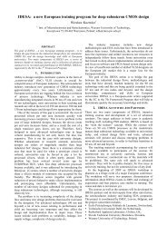
24-26 September 2008, Rome, ItalyCFD for Electronics Cooling: MCAD and <strong>EDA</strong>Embedded vs. Stand-aloneJohn D. ParryMentor Graphics Corporation Mechanical Analysis Division81 Bridge Road, East MoleseySurrey, KT8 9HH, UKAbstract–Computational Fluid Dynamics (CFD) forElectronics Cooling (EC) has developed differently fromgeneral-purpose CFD, due to the nature of the market it serves.The benefits are clear – the use of EC CFD in product designhas had a profound impact on both time-to-market and cost.Today the EC CFD market is dominated by suites ofapplication-specific codes, focused at the different packaginglevels: system-, board- and package-. Their usage maps ontocurrent product design flows at different stages in the productcreation process, from IC package to equipment design.Interfacing with <strong>EDA</strong> and MCAD software has helped theirincorporation into existing in-house design practices. MCADembeddedCFD software is gaining popularity and being soldeffectively by MCAD vendors for general-purpose applications.<strong>EDA</strong> vendors are again taking an interest in thermal design.This invited paper considers the future of EC CFD and theprospects for stand-alone software vs. mechanical CADembeddedand <strong>EDA</strong>-embedded solutions. This is considered inthe context of how today’s EC market has developed over time,and the unique requirements placed on EC CFD tools.The challenges of both MCAD and <strong>EDA</strong> embedded EC CFDare discussed from both technical and business standpoints.I. INTRODUCTIONIt’s worth reflecting on the impact EC CFD has had on thethermal design of electronic products. Companies that useEC CFD have been independently found to complete thermaldesign verification almost 3 times faster than those thatdon’t, as shown in Fig. 1 [1].To get an understanding of how this has been achievedand the prospects for the future, we need to look at howtoday’s EC CFD market has developed.II. HISTORY OF CFD IN ELECTRONICS COOLINGWhat follows is by nature anecdotal, being unavailable asarchival material, but comes from the memories of severalpeople involved with EC CFD from the outset. It is anabridged version of events, presenting only what is mostpertinent to the topic of this paper, in roughly chronologicalorder.1970s & 80s: 1974 saw the foundation of CHAM Ltd., thefirst commercial company to provide a CFD consultancyservice, and later software, to industry. PHOENICS debutedin 1981 as the first commercially available software tool inCFD [2]. Electronic Design Automation also dates back tothe beginning of the 1980s, when Daisy Systems, MentorGraphics Corporation and Valid Logic Systems were allformed. Creare Inc. launched the first version of Fluent in1983. The use of commercial CFD codes in electronics datesback to the mid to late 1980s when Dereje Agonaferintroduced a number of licenses of PHOENICS into IBMPoughkeepsie. At around the same time Fluent from Crearewas being used by DEC. The mid 1980s saw rapid growth inchip power in the bipolar-based digital circuitry of the day,as Fig. 2 shows [3]. The mid to late 1980s saw theemergence of PCB thermal design tools. One of the first wasPCBTHERMAL from Pacific Numerix.% Design time spent on ThermalVerificationFig. 1: Proportion of Total Design Time taken to Verify Thermal DesignFig. 2: Growth of Bipolar and CMOS Module Heat Flux©<strong>EDA</strong> <strong>Publishing</strong>/THERMINIC 2008 1ISBN: 978-2-35500-008-9
24-26 September 2008, Rome, Italy<strong>EDA</strong> companies also started to produce or market theirown offerings. Mentor Graphics produced AutoTherm,Cadence acquired and marketed Thermax, and Racal-Redac,now part of Zuken Inc., produced VTAT and later theirThermal Placement tool. The mid 1980s also saw the birth ofthe first CFD code dedicated to EC when J. P. Bardon(CNET, France) presented THEBES at the ASME IHTconference in San Francisco in 1986. An English versionIII.became available in 1987 and was extensively tested byPhilips for consumer electronics applications [4]. During1988 Fluent Inc. was spun off from Creare, and FlomericsLtd. was founded. FloTHERM made its debut in late 1989.1990s: In 1992, newly-founded Blue Ridge Numerics Inc.released CFDesign, a general-purpose CFD solution tightlyintegrated with MCAD software, and Daat Research Corp.,who’s flagship product, Coolit is targeted at EC applications,was founded. In 1994, taking inspiration from FloTHERM,Fluid Dynamics International (FDI) released the first versionof IcePak based on its FIDAP FE solver with the userinterface written by ICEM-CFD Engineering, now a part ofANSYS Inc.; Mentor Graphics acquired Thebes, which wasymarketed as AutoFlow; and Harvard Thermal was founded,releasing its Thermal Analysis System (TAS), a conductionand radiation tool for military and defense applications. InAugust 1995, Fluent Inc. was acquired by Aavid ThermalTechnologies, Inc. In May 1996, Fluent acquired FDI, and in1997 Fluent released the first version of IcePak based on theFluent UNS solver. In 1998 Flomerics launched FloPACK, aweb-based application creating thermal models of chippackages and other electronics parts for use in FloTHERM.In 1999 Flomerics released the Command Center to controland co-ordinate distributed processing of multiple jobssimultaneously across a large heterogeneous network, andNika GmbH was founded, producing the first MCADembeddedCFD product, Floworks, marketed by SolidWorksCorp. under the COSMOS brand.2000s: Aavid was purchased by Willis Stein & Partners, aUS private equity investment firm in January 2000. In 2002Harvard Thermal began shipping TASPCB aimed at PCBdesigners and incorporating a CFD capability. In January2004 Future Facilities formed as a spin-off from Flomericsto market FloVent to the data center market. Flomericsreleased FloPCB and Nika’s Engineering Fluid DynamicsYour case(EFD) software became available for CATIA V5, when andtemperatures willlater the same year Fluent released Iceboard. In early 2005be...Fluent released Icechip, Flomerics acquired HungarianbasedMicReD in May to provide model validation andtesting services, Nika released EFD.Pro for Pro/ENGINEERin June and Daat released CoolitPCB in July. 2006 saw therelease of FloPCB for Allegro by Flomerics. In May Fluentwas acquired by ANSYS Inc. and in June Nika GmbH wasacquired by Flomerics. Mentor Graphics acquired theBETAsoft product line in May 2007, which previously wasdeveloped, sold, and supported by Dynamic Soft Analysis,T j = 78°Cand is now marketed by Mentor as HyperLinx Thermal. InDecember Flomerics released its electronics-specific modulefor EFD. In June 2008 Flomerics released ThermPaq,extending FloPACK’s compact thermal model generationcapability to complete packaged chip characterization forautomated generation of package metrics. At the time ofwriting, Flomerics have just been acquired, becomingMentor Graphics’ Mechanical Analysis Division.The picture is then one of first innovation with newcompanies and new products from existing companiesemerging onto the market and later consolidation throughacquisition.OBSERVATIONS FROM HISTORYPrior to the introduction of CFD, mechanical engineersoften relied on the use of metrics such as θ JA and θ JC in handcalculations to estimate component temperature rises. Suchmetrics, particularly θ JA , include a contribution from the testenvironment. Consequently they are not well suited fordesign, which is now widely recognized [5]. As the heattransfer coefficient in the application is unknown, thermaldesign of complex air cooled systems becomes guesswork,as humorously depicted by Kromann & Argento (Motorola)in Fig. 3.Early use of EC CFD was focused on system-level designverification when physical prototypes became available.Problems, when found, led to costly late-cycle redesign asdepicted in Fig. 4. Early <strong>EDA</strong>-integrated thermal tools usingcorrelations for the air-side heat transfer were the maincompetition for CFD during the early 1990s. Lack of thermaldata and an inability to accurately represent the air side heattransfer limited their suitability for system-level analysis,although reports of their use can still be found [6, 7].Major general-purpose CFD codes like PHOENICS,Fluent, Star-CD had been around for some time when the useof EC CFD started to gather pace. They found relativelylittle use within this market sector, held back by the lack of aconjugate heat transfer capability and time consuming meshgeneration. Burdick [8] comments that “A small number ofengineers attempted to use commercially available generalpurpose finite-difference CFD programs at this time but theresult of several months of activity was usually fruitless”.The lack of useful data for system-level thermal designgave rise to research into models that capture the thermaland flow behavior of many of the components found inelectronics systems.Θ ja = (T j - T a )/P chip => Θ ja = 18.5 °C/WT j = Θ ja P chip + T rise + T ambientwhere, Θ ja = Θ jc + Θ caΘ ja70°C80°C90°CPWB TemperatureFig. 3: Equally Valid Design Practices if h is Unknown©<strong>EDA</strong> <strong>Publishing</strong>/THERMINIC 2008 2ISBN: 978-2-35500-008-9
ElectronicDesignMechanical/ThermalDesignConceptPoor integration /Limited communicationDetailed DesignPrototypeValidationToo much late-cycleredesignTestFig. 4: Typical thermal design process (circa 1990)ActualCostBudgetedCostFlomerics’ in-house Package Level Thermal Initiative(PLTI) in the early 1990s preceded two successfulEuropean-funded projects which Flomerics coordinated:DELPHI [9] and SEED [10] with a subsequent projectPROFIT, coordinated by Philips Research [11]. Theseprojects led to the concept of Boundary ConditionIndependence (BCI) for models of parts such as axial fans,various chip packages families, and heat sinks. The CompactThermal Models (CTMs) of chip packages that resulted fromthis work has since given rise to substantial additionalresearch, and standardization efforts in this area have nowborne fruit [12, 13]. The market quickly became heavilydominated by stand-alone electronics-specific system-levelcodes like FloTHERM and later Icepak.The early focus on telecoms, computing and laternetworking continued from the outset until 2000 when the‘dot com’ bubble burst and design work in these industriesall but stopped as equipment remained unsold in warehouses.Sectors such as defense, aerospace and automotive came tothe fore, placing increased emphasis on links to mechanicalCAD systems.Early system-level EC CFD software was complementedby product offerings at first board and then package levelproviding suites of software that share models and map ontomuch of the electronics design flow. FloPACK is anexception to this general trend, but its early appearanceresulted in part from the research noted above. Increasinguse at board-level to predict junction temperatures fueledconcerns over predictive accuracy motivating numerousinvestigations into the performance of Reynolds-AveragedNavier-Stokes (RANS) turbulence closure models for thisclass of flow [14, 15].Fig. 5: QFP Package and Corresponding Compact Thermal Model ShowingLinks24-26 September 2008, Rome, ItalyLimitations in computing power and short design timespreclude the use of more advanced transient techniques likeLarge Eddy Simulation (LES) for electronics product design.Despite accuracy concerns, the use of zero-equation RANSmodels with first-order differencing schemes on hexdominatedmeshes remains the technology of choice [16].Today, stand-alone electronics-specific software remainsdominant. To understand why the market has evolved thisway it’s necessary to examine the unique requirements ECplaces on CFD software.IV. UNIQUE FEATURES OF THE ELECTRONICS COOLINGMARKETOne of the first industries to embrace CFD was theaerospace industry. Early Eulerian solvers pioneered the use ofstructured body-fitted meshes for transonic flows lead the laterfinite-volume Navier-Stokes solvers down a body-fitteddevelopment trajectory [17]. The need to handle morecomplex, sometimes moving geometries led to thedevelopment of fully unstructured body-fitted codes and meshgenerators. Support for user-created coding allowed researchscientists to apply CFD to a variety of industrial problems andthese developments have fed into the general-purpose CFDsoftware of today. Typically used by professional analysts witha strong background in fluid dynamics and numerical methods,these tools are capable of handling free-surface flows,combustion and chemical reaction, multi-phase phenomena andmuch more.In EC, the early adopters were the experienced thermalengineers that worked through the bipolar age with a strongbackground in measurement techniques gained through buildand-testprototyping. Mainly mechanical engineers (MEs), plusthe odd physicist, they were converted to using CFD by theinsights it provided into system-level air flow. Theirknowledge helped direct and drive the software development.The need for robustness in terms of solution convergencerapidly became clear, removing the burden of knowledge aboutthe numerical aspects of CFD that would otherwise be neededto take effective remedial action. MEs with some knowledge ofheat transfer but no CFD expertise remains the target userprofile for EC CFD.What makes EC applications challenging is the sheernumber of discrete objects that make up a typical problem; thedifference in length scales from chip to system; the need forconjugate heat transfer and surface-surface radiation. Finally,the complex flow and thermal characteristics of many of thecomponent parts that make up an electronics system: chippackages, fans, heat pipes, thermoelectric coolers (TECs), etc.,need to be represented without the user needing knowledge ofhow to model these. Providing parameterized behavioralmodels of cooling components presents a major challenge toCFD vendors addressing the EC market and acts as a barrier toentry.Flows are often transitional, with turbulence created by flowover the many small components present in the system, yet asolution has to be obtained in hours at most on a desktopcomputer. As a result, unique technologies have appeared, suchas locally embedded fine meshes to help address the disparityin length scales.©<strong>EDA</strong> <strong>Publishing</strong>/THERMINIC 2008 3ISBN: 978-2-35500-008-9
Staggered Cartesian meshes tolerate very high cell aspectratios (e.g. 100:1) without impacting result quality, makingthem efficient at handling thin layered structures like PCBs,heat sink fins, etc.Libraries of behavioral models of common parts, such asfans, heat sinks, chip packages, etc. have an important role toplay in efficiently creating a thermal model of an electronicsenclosure. Some progress has been made in getting suppliersto provide flow/thermal models of the parts they sell, notablyheat sinks, fans, filters, interface materials, typical ICpackages and TECs [18]. Heat sinks were one of the firstparts to become available, but the requirement to customizedesigns for each application has since reduced this need.Today heat pipes are a common feature in many products,with liquid cooling being employed in some applications.These and future cooling technologies such as synthetic jets[19] and piezo fans [20] are expected to lead to an increasedemphasis on validated libraries of parts.Cooling adds cost, weight and volume to electronicsproducts generally without improving functionalperformance. The desire to minimize cooling costs against abackground of increasing thermal density has led to anemphasis on design optimization. Early efforts were focusedwas on fan and vent positioning to improve flowdistribution. As space constraints and power densitiesincreased, heat sink optimization became important tominimize weight, system pressure drop and wake effects.The Cartesian nature of the geometry, use of Cartesianmeshes, and robust solution techniques support fullyautomatedexploration of the design space. Addition,movement and removal of objects coupled with space-fillingDesign-of-Experiment (DoE) techniques with objectcollision detection and optimization techniques makes itpossible to optimize component placement, PCB spacing,heat sink design, etc.Over the last 20 years EC CFD codes have had their owndevelopment trajectory, quite different to that of general-24-26 September 2008, Rome, Italypurpose CFD, driven by the needs of a different target userprofile. As electronics products and the cooling technologiesthey employ continue to miniaturize, new challenges willappear: micro-channel cooling pushes the limits ofapplicability of the Navier-Stokes equations requiring a slipcondition at wall boundaries, and the design of MEMSdevices often requires a multi-physics approach. Vendors ofLattice Boltzmann method codes have also shown an interestin EC.Fig. 6: Local Embedded Fine CFD GridV. ELECTRONICS COOLING CFD: CAUGHT BETWEENMCAD AND <strong>EDA</strong>For EC applications, CFD sits at the interface between theMCAD and <strong>EDA</strong> worlds. A CFD model of a completeelectronics enclosure contains both mechanical andelectronic parts, and so needs information from both theseworlds. By the end of the design process, part details anddesign powers, PCB layout, details of the board structure etc.are all available within the <strong>EDA</strong> system. However, due tothe largely 2D nature of electronics design, necessarymechanical information about the board assembly is oftenlacking, such as component height.The geometric detail of almost all other aspects of theproduct will exist within the MCAD system. Neither systemcontains information about the thermal properties of thematerials used in the product, nor do they contain behavioralmodels of the parts needed for the analysis, such asresistance networks for packages, fan curves, heat pipeeffective thermal resistance, TEC performance data, etc. orinformation about the product’s operating environment,needed to define boundary conditions for the analysis.VI. THE CASE FOR STAND-ALONE EC CFDIn general, building geometry within a CFD pre-processoris a lot less efficient than using a modern feature-basedMCAD tool to do the same job. However, stand-alone ECCFD has served the industry well. In the early days, limiteddesktop computing power forced significant modelsimplification. The experienced thermal engineers that firstadopted EC CFD created models manually and were capableof making appropriate simplifying assumptions andproviding representative values for any missing data. ECCFD pre-processors handled the historically-Cartesianelectronics geometries well, so models could be easilyevolved as more information about the design becameavailable and refined where indicated by thermal concerns.In many EC applications the geometry is still largelyCartesian, or can be treated as such. Creation of suchgeometry as a pre-processing step within the EC CFD toolremains efficient.Today stand-alone tools are heavily supported bysophisticated interfacing software that can import MCADgeometry in various formats like STEP and ACIS SAT.Geometry can be ‘healed’ to remove small gaps, simplifiedand adapted for analysis, for example by replacing theMCAD assembly for an axial fan with the equivalentbehavioral model from a library with just a few mouseclicks.©<strong>EDA</strong> <strong>Publishing</strong>/THERMINIC 2008 4ISBN: 978-2-35500-008-9
24-26 September 2008, Rome, ItalyConceptDetailed DesignValidationElectronicDesignPrototypeTestActualCostMechanical/ThermalDesignBudgetedCost8-10 weeks potentialtime saving per projectSeveral redesignseliminatedFig. 8: Thermal Design Process using CFD during Conceptual DesignFig. 7: CAD Fan Assembly ReplacementStand-alone board-level EC CFD tools have sophisticatedbidirectional interfaces that allow filtering on componentsize, power, power density etc., with back-annotation ofcomponent placement to the <strong>EDA</strong> system. This makes itpossible for thermal design to influence the <strong>EDA</strong> designflow, reducing board re-spins in late design and the numberof physical prototypes needed, saving weeks during design.These stand-alone board-level tools facilitate collaborationbetween product marketing, EEs and MEs on the PCBdesign, particularly during the conceptual phase of thedesign process. But who will actually use them? Experienceto date has shown that the users of board-level EC CFD toolsare more likely to be MEs than EEs, despite many attemptsby many vendors to encourage EEs to perform board-levelthermal analysis.Most thermal engineers come from a mechanical ratherthan electrical background, but are not necessarily designers,and so are not proficient users of MCAD software. They areoften a scarce resource within their organizations. For them,stand-alone EC CFD software, supported by sophisticatedMCAD and <strong>EDA</strong> interfaces arguably provides the bestanalysis platform.VII. THE CASE FOR <strong>EDA</strong>-EMBEDDED EC CFDThe case for <strong>EDA</strong>-embedded EC CFD is predicated on theassumption that it is possible to package the technology sothat it can be used effectively by EEs, reducing reliance onthe MEs they heavily outnumber. For significant EE usage tobecome a reality it will be necessary to embed EC CFDwithin the <strong>EDA</strong> software EEs are used to using, and at thesame time design the software to have a very high level ofautomation so very little heat transfer knowledge is required.Solutions at board and package level could be embeddedin the different tools within the <strong>EDA</strong> suite. At chip level,electro-thermal simulation is needed [21] to account for thelocal effect on leakage current and hence power dissipation,but needs as boundary conditions the thermal environmentrepresented by the package, PCB and heat sink. Some workhas been done in this area [22], but the main benefit of CFDis being able to predict air flow, making it most suited forboard-level tools.For a specific packaging level such as board-level, outputcan be simplified to enable the user to determine whetherthere are any thermal issues with their design, reportingcomponents that exceed their maximum specified junction orcase temperatures for a pre-defined environment like a cardslot.The main benefit of possible future <strong>EDA</strong>-embedded ECCFD is that its use model would enable thermal analysis tobe done earlier in the electronics design flow, influencingplacement, routing, and the introduction of thermal vias, etc.A pre-requisite for this is the availability, either within the<strong>EDA</strong> system, or through libraries it addresses, of theadditional geometric data needed to create a 3Drepresentation of the PCB such as the physical extents andlocation of chip packages and thermal models of thosepackages.The value proposition for <strong>EDA</strong>-embedded EC CFD isclear, and the creation of such software is challenging buttechnically feasible. There is also sufficient need, as thermaldesign considerations require layout and architecturalflexibility for heat sinking, etc. The 2007 ITRS Roadmap onAssembly and Packaging states that the use of massive aircooledheat sinks “limits the chip packing density inelectronic products thereby increasing wiring length, whichcontributes to higher interconnect latency, higher powerdissipation, lower bandwidth, and higher interconnectlosses.”<strong>EDA</strong> vendors have previously demonstrated their abilityto bundle board-level thermal tools through their normalsales channels. Correctly packaged, it should be possible for<strong>EDA</strong> vendors to bundle a CFD-based thermal module as partof a suite of <strong>EDA</strong> software, accessing a market that isunavailable to CFD vendors. CFD vendors have shown thatCFD technology can be ‘packaged’ to the point where it isinvisible to the user, so the creation of <strong>EDA</strong>-embedded ECCFD is both technically and commercially feasible.Whilst <strong>EDA</strong>-embedded EC CFD is attractive, their usemodel requires a shift in thermal design work from MEs, to asharing with the EEs using the <strong>EDA</strong>-embedded software.There is a risk that such tools, if produced, will not gainwidespread acceptance, unless good thermal design canassured by MEs retaining overall responsibility for thisaspect of the physical design.©<strong>EDA</strong> <strong>Publishing</strong>/THERMINIC 2008 5ISBN: 978-2-35500-008-9
VIII. THE CASE FOR MCAD-EMBEDDED EC CFDMCAD-integrated and embedded solutions appeared inthe early 1990s and have been recently reported to be thefastest growing segment of the overall CFD market. Theyhave a smaller share of the EC market than stand-alone tools,but EC remains an important application area.MEs graduating today are almost certain to be proficientusers of 3D MCAD software, which has been available insome high schools for almost a decade [23]. In industryMCAD tools are being used from the concept design stage atthe start of the mechanical design process. New electronicproducts often re-use electronic and mechanical parts fromthe previous generation, so geometry that already exists inthe MCAD system forms a natural starting point. Formechanical reasons, such as interference checking, MCADsystems can already import a full geometric representation ofthe board from the <strong>EDA</strong> system. CircuitWorks is a bidirectionalIDF and PADS file interface for the SolidWorks3D CAD system for example [24].CFD vendors have shown that it is possible to embed CFDinto MCAD environments and provide useable facilities toinput the additional data etc. needed for the analysis and postprocess the results. SolidWorks Corp. and ParametricTechnology Corp. amongst others, have shown that MCADsuppliers are able to effectively market and sell sophisticatedFEA and CFD software through their direct and reseller saleschannels. All the necessary ingredients are available to adaptMCAD-embedded CFD for the EC market. As such,MCAD-embedded EC CFD offerings are a certainty.The suitability of CAD models for analysis remains apoint of contention [25, 26]. CAD models created formanufacturing typically contain a lot of detail such asthreads, seals, fillets, rounds, etc and have tolerances thatallow assembly, that can cause problems for analysis tools.From an analysis perspective the CAD model is oftenconsidered ‘dirty’ due to its lack of watertightness, whereasit was created for a quite different purpose. CAD ‘cleanup’(and simplification) is a recognized process step in generalpurposeCFD but can be time consuming, so it is tempting totry to keep these simplified copies up to date rather than reexportand clean up the manufacturing CAD model as thedesign progresses. However, this leads to ‘versionitis’ as thecopies become stale, and undetected differences creep in. Ifthe intention is to check the performance of a design beforecommitting to manufacturing it, a better approach is to firstcreate simplified parametric CAD models that are bothappropriate for the analysis and easy to modify. Early in thedesign process a ‘Design for Analysis’ paradigm is needed,with focus shifting to ‘Design for Manufacture’ only afterthe design’s performance is proven to be satisfactory.IX. CONCLUSIONSDesign practices tend to change slowly, driven by costreduction rather than the availability of innovative tools.Stand-alone tools will therefore be around for some time tocome. They work very well, companies have built their useinto their design flows and the MEs that use them have builtrelationships with EEs to obtain the data they need for theanalysis, facilitated by interfacing software. MCAD-24-26 September 2008, Rome, Italyembedded EC CFD effectively exists today [27]. Substantialimprovements are expected as future developments furtheraddress the unique and changing needs of the EC market.MCAD-embedded EC CFD entrenches the responsibility forthermal design within the ME community.Perhaps the greatest hope for the future of electronicsthermal design lies not in MCAD or <strong>EDA</strong> embeddedproducts as point solutions, but in broader electronic andmechanical co-design. Successful products are defined bythe user experience in terms of aesthetics, ergonomics andfunction. The product’s form is no longer defined by theelectronics it houses. Keypads and touch screens blur thedistinction between casing and electronics and hence thedistinction between the MCAD and <strong>EDA</strong> worlds. A singlecommon design environment is impractical, but 3Dmodeling in <strong>EDA</strong> would facilitate bidirectional notificationof relevant design changes and data exchange betweensystems. Progress is already being made in this area, drivenby the need for interference checks, etc. as products continueto miniaturize. As the <strong>EDA</strong> and MCAD worlds converge thepotential for communication between EC CFD toolsembedded within these design environments increases, andso may be expected to happen over time.What is clear is the importance of thermal design isunlikely to diminish as companies strive to achieve costeffectivedesigns whilst power densities in high performanceapplications continue to increase, driving innovations incooling technology and design practices. Developments inEC CFD software will need to keep pace with theseinnovations to meet the future challenges and opportunitiespresented by this changing market.ACKNOWLEDGMENTI’m grateful to Drs. David Tatchell, Clemens Lasance, IanClark and Robin Bornoff for their comments and suggestionsfor improving this manuscript. All trademarks used in thispaper are recognised as property of their respective owners.REFERENCES[1] “Electronics – Correct by Design”, Benchmark Report, AberdeenGroup, 2007[2] Dr. Akshai K. Runchal, “Brian Spalding: CFD & Reality”, Proc. ofCHT-08, May 11-16, 2008, Marrakech, Morocco (CHT-08-012)[3] Kaveh Azar, “The history of power dissipation”, ElectronicsCoolingMagazine, Vol. 6, No. 1, pp. 42-50, January 2000[http://electronics-cooling.com/articles/2000/2000_jan_a2.php][4] Clemens J.M. Lasance, “20 Years of CFD for thermal managementat Philips Electronics”, Proc. of Theta Workshop, Cairo, January 6,2007[5] Integrated Circuits Thermal Test Method Environment Conditions -Natural Convection (Still Air) EIA/JEDEC STANDARDEIA/JESD51-2. [http://www.jedec.org/download/search/jesd51-2.pdf][6] “Mentor Graphics Announces Winners of its 19th Annual PCBTechnology Leadership Awards” 28 Mar. 2007 [CIMdata PLMIndustry Summary, Vol. 9 No. 13, 30 Mar. 2007].[http://www.cimdata.com/newsletter/2007/13/documents/Mar07CIS30.pdf][7] Weiping Jing, Xiaochun Wu, Ling Sun, “An application of MCMtechnology”, Proc. of 6th EPTC, Sept. 2005, pp. 117-120.[8] J. S. Burdick, “Electronics Cooling at IBM Endicott”, Proc. of 1stFloTHERM Int. User Conf., Guildford UK, Sept. 1991, pp. 53-77.[9] Harvey Rosten, et al., “Final Report to SEMITHERM XIII on theEuropean-Funded Project DELPHI - the Development of Librariesand Physical Models for an Integrated Design Environment”, Proc.©<strong>EDA</strong> <strong>Publishing</strong>/THERMINIC 2008 6ISBN: 978-2-35500-008-9
24-26 September 2008, Rome, Italyof IEEE SEMITHERM XIII, 20-30 Jan. 1997, pp. 73-91.[10] H. Pape, G. Noebauer, “Generation and verification of boundaryindependent compact thermal models for active componentsaccording to the DELPHI/SEED methods”, Proc. of IEEESEMITHERM XV, San Diego, Mar. 1999, pp. 201-211.[11] C.J.M. Lasance, “The European project PROFIT: prediction oftemperature gradients influencing the quality of electronicproducts”, Proc. of IEEE SEMITHERM XVII, San Jose CA, March2001, pp. 120-125.[12] Two-Resistor Compact Thermal Model Guideline, EIA/JEDECSTANDARD JESD15-3.[http://www.jedec.org/DOWNLOAD/search/JESD15-3.pdf][13] DELPHI Compact Thermal Model Guideline, EIA/JEDECSTANDARD JESD15-4.[14] Rodgers, P., Eveloy, V., and Davies, M., “An ExperimentalAssessment of Numerical Predictive Accuracy for ElectronicComponent Heat Transfer in Forced Convection: Parts I and II”,Trans. of ASME JEP, Vol. 125, No. 1, 2003, pp. 67-83.[15] K. Dhinsa, C. Bailey, K. Pericleous, “Investigation into theperformance of turbulence models for fluid flow and heat transferphenomena in electronic applications”, IEEE Trans. on Comp. andPack. Tech., Vol. 28, No. 4, Dec. 2005, pp. 686-699.[16] Emre Ozturk and Ilker Tari, “CFD Modeling of Forced Cooling ofComputer Chassis”, Eng. App. of Comp. Fluid Mech., Vol. 1 No. 4,pp. 304-313, 2007.[http://www.cse.polyu.edu.hk/publication/jeacfm/][17] W. N. Dawes, “Turbomachinery computational fluid dynamics:asymptotes and paradigm shifts”, Phil. Trans. of R. Soc. A (2007)Vol. 365, pp. 2553–2585.[18] [www.SmartParts3D.com][19] Raghav Mahalingam, Sam Heffington, Lee Jones and RandyWilliams, “Synthetic Jets for Forced Air Cooling of Electronics”,ElectronicsCooling Magazine, Vol. 13, No. 2, May 2007, pp. 12-18.[http://electronics-cooling.com/articles/2007/may/a1/][20] Ioan Sauciuc, “Piezo actuators for electronics cooling”,ElectronicsCooling Magazine, Vo. 13, No. 1, Feb. 2007 pp. 12-17.[http://electronics-cooling.com/articles/2007/feb/a1/][21] András Poppe, György Horváth, Gergely Nagy, Márta Rencz andVladimír Székely, “Electro-thermal and logi-thermal simulatorsaimed at the temperature-aware design of complex integratedcircuits”, Proc. of 24th IEEE SEMI-THERM Symposium, San JoseCA, March 2008, pp. 68-76.[22] “Co-simulation of the Die and the Package”, [http://www.gradientda.com/part/flomerics.htm][23] “A brief outline of the CAD/CAM in Schools programme”,[http://www.cadinschools.org/][24] [www.priware.com][25] Ivo Weinhold, “The 5 Myths of CFD”, NAFEMS BENCHmarkMagazine, April 2008, pp. 28-29.[26] Althea de Souza, “CFD Mythology”, NAFEMS BENCHmarkMagazine, June 2008, pp. 23-24.[27] “Flomerics Releases Version 8.1 of EFD Engineering FluidDynamics Analysis Software”http://www.flomerics.com/industries/details_news.php?id=1275©<strong>EDA</strong> <strong>Publishing</strong>/THERMINIC 2008 7ISBN: 978-2-35500-008-9
24-26 September 2008, Rome, ItalyTriangulation Method for Structure Functions ofMulti-Directional Heat-FlowsLorenzo Codecasa, Dario D’Amore, Paolo MaffezzoniPolitecnico di Milano, Milan, Italye-mail: {codecasa, damore, pmaffezz}@elet.polimi.itAbstract— In this paper previous results proposed by theauthors for localizing defects in components and packages bymeans of structure functions in three-dimensinal heat diffusionproblems have been generalized. To this aim a novel traingulationapproach is presented based on the use of structure functionscorresponding to dinstinct heat sources.I. INTRODUCTIONStructure functions have been originally used by V. Székeyet. al. as means for inferring on the spatial distributions ofthermal properties in one-directional heat flows [1]. Precisely,a 1-D heat diffusion problem in which power is injected atone boundary and temperature rise is measured at the sameboundary, referred to as one-directional heat flow, definesa short-circuited RC transmission line. This short-circuitedRC transmission line is characterized by a structure function,relating the cumulative thermal resistance and capacitancealong the line. Such structure function can be determined fromthe port response of the short-circuited RC transmission line,by solving an inverse problem. In this way information on thespatial distribution of thermal properties are recovered fromthe port response of a one-port dynamic thermal network.For the general case of a one-port passive dynamic thermalnetwork modeling a 3-D heat diffusion problem, referred toas multi-directional heat flow, the authors have shown in [2]that a structure function can still be defined and in [3] thata relation exists between structure function and the spatialdistribution of thermal properties.In this paper such results on structure functions are exploitedand a novel method, based on triangulation, for spatiallylocalizing defects in components and packages is provided. Asshown by the authors in [3], for a given heat source, and forthe corresponding one-port passive dynamic thermal network,the values of the structure function up to a given value of thecumulative thermal resistance R and capacitance C dependsby all and only the values of the thermal conductivity andvolumetric heat capacity within a given spatial region Ω. Theboundary of Ω is solution of an eikonal equation [3]. Thisfact suggests the following procedure for localizing defects bymeans of structure functions. Let C be a reference componentor package whose spatial distribution of thermal propertiesis known and let C 1 be a component or package presentingdefects in the spatial distribution of thermal properties withrespect to C.LetC(R) and C 1 (R) be respectively the structurefunctions of C and C 1 , with respect to a given heat source.By comparing the structure functions C(R) and C 1 (R) andby evaluating the smallest values of C and R at which theydiffer, the region Ω in which no defects are present can bedetermined by solving an eikonal equation.However in this way only a raw localization of a defects canbe in general achieved. Accurate localizations are shown to bein general feasable by repeating this procedure with respect todifferent heat sources. This approach has been numericallyimplemented. To this aim the well known Fast MarchingMethod [4] has been used for solving the eikonal equation,in order to determine the boundaries of the regions withoutdefects. Using the implemented numerical method, accuratelocalizations of defects have been achieved in a referenceexample.The remaining of this paper is organized as follows. Insection II structure functions for generic three-dimensionalheat diffusion problems are recalled. In section III the relationbetween spatial distributions of thermal properties and structurefunctions in described. The novel triangulation approachis presented in section IV. Examples of localization of defects,both analytical and numerical are presented in sections V andVI respectively. .II. STRUCTURE FUNCTIONS OF Multi-Directional HEATFLOWSAs it has been shown by the authors [2], structure functionscan be introduced for one-port passive dynamic thermalnetworks modelling generic three-dimensional heat diffusionproblems. Precisely, let us consider a three-dimensional heatdiffusion problem in a bounded spatial region Ω, referred to asmulti-directional heat flow. The relation between the generatedpower density G(r,t), the temperature rise distribution u(r,t)and the heat flux density q(r,t) is ruled by the First Principleof Thermodynamics and by Fourier’s law as follows∇·q(r,t)+c(r) ∂u (r,t)=G(r,t), (1)∂tq(r,t)=−k(r)∇u(r,t), (2)in which c(r) is the volumetric heat capacity and k(r) isthe thermal conductivity. Conditions on the boundary ∂Ω,assumed of Robin’s type, areq ν (r,t)=h(r)u(r,t), (3)in which h(r) is the heat transfer coefficient, ν(r) is the unitvector outward normal to ∂Ω and q ν (r,t)=q(r,t) · ν(r).Initial condition is assumed to be zerou(r, 0) = 0. (4)©<strong>EDA</strong> <strong>Publishing</strong>/THERMINIC 2008 8ISBN: 978-2-35500-008-9
24-26 September 2008, Rome, ItalyA one-port passive dynamic thermal network N can bedefined as in [2], [5], [6], by introducing the power P (t) andthe temperature rise T (t) measured at its port as follows. Thepower P (t) determines the power density G(r,t) asG(r,t)=g(r)P (t) (5)in which g(r) is a chosen function whose support is Σ. Thetemperature rise T (t) is a weighted mean of u(r,t) definedby∫T (t) = g(r)u(r,t) dr. (6)ΩThe natural means for characterizing the port response ofthis one-port passive dynamic thermal network is the powerimpulse thermal response z(t), in the time domain, and thethermal impedance function Z(s), in the complex angularfrequency domain. Moreover, as proven in [2], N can bemodelled by a short-circuited RC transmission line. Suchan RC transmission line can be ruled by is it characterizedby a structure function C(R) in which R and C are thecumulative resistance and capacitance along the line. Thestructure function, as shown in [2], can determined from theport response of N . In fact by solving for Z(C, s) the Riccatitypeequation∂Z∂C (C, s) − s Z2 (C, s) = ∂Z (C, 0). (7)∂Cwith boundary conditionthe R(C) function is recovered asZ(0,s)=Z(s) (8)R(C) =Z(0) − Z(C, 0) (9)from which, by inverting R(C), the structure function C(R)is obtained.III. RELATION BETWEEN SPATIAL DISTRIBUTIONS OFTHERMAL PROPERTIES AND STRUCTURE FUNCTIONSAs shown in [3], the relation between the structure functionof a one-port passive dynamic thermal network and the spatialdistribution of thermal properties in multi-directional heat flowcan be established. in terms of a companion wave propagationproblem and a one-port lossless network. The wave propagationproblem, in the unknown variables v(r,t), j(r,t), isdefined in Ω as follows∇·j(r,t)+c(r) ∂v (r,t)=G(r,t), (10)∂t∂j(r,t)=−k(r)∇v(r,t) (11)∂twith boundary conditions on ∂Ω,∂j ν(r,t)=h(r)v(r,t), (12)∂tbeing j ν (r,t)=j(r,t) · ν(r), and initial conditions in Ω,v(r, 0) = 0, (13)j(r, 0) = 0. (14)The spatial distributions c(r), k(r) and h(r) are common to theheat diffusion problem and to the wave propagation problem.The one-port lossless network N LC is obtained from thewave propagation problem by defining the current I(t) and thevoltage V (t) measured at its port. The current I(t) determinesG(r,t) asG(r,t)=g(r)I(t). (15)The voltage V (t) is∫V (t) =Ωg(r)v(r,t) dr. (16)The relation between the current I(t) and the voltage V (t) isrepresented, in the time domain, by the impulse response functionz LC (t) and, in the complex angular frequency domain, bythe impedance function Z LC (s). It results inZ LC (s) =s Z(s 2 ). (17)Thus, since N can be modelled by a short-circuited RCtransmission line, as recalled in Section II, then from thetheory of linear circuits it descends [7] that N LC can bemodelled by a short-circuited LC transmission line obtainedfrom the short-circuited RC transmission line modelling N bysubstituting all resistive elements with inductive elements.The short-circuited LC transmission line is characterized bya structure function which coincides with the structure functionof the short-circuited RC transmission line modelling N .Thus the C(R) structure function characterizes not onlyN LC but also N .The relation between the structure function of the one-portpassive dynamic thermal network and the spatial distributionof thermal properties is established by defining the relationbetween the material properties c(r), k(r) and h(r) of thewave propagation problem and the structure function C(R) ofthe one-port lossless network N LC .Let v(r,t), j(r,t) be the solution of the wave propagationproblem in response to a unit impulse I(t). Letω c (τ 1 ) be thesub-region of Ω in each r of which v(r,t) ≠0at some t ≤ τ 1and let ∂ω k (τ 1 ) be its boundary. Similarly let ω k (τ 1 ) be thesub-region of Ω in each r of which j(r,t) ≠ 0 at some t ≤ τ 1and let ∂ω k (τ 1 ) be its boundary.The ω c (τ 1 ) and ω k (τ 1 ) regions can be characterized asfollows. The ω c (0) region is the support of v(r, 0). Sincefrom Eqs. (10)-(13) it is v(r, 0) = g(r)/c(r), ω c (0) is theregion Σ in which power is generated. Similarly ω k (0) is thesupport of j(r, 0), which is a sub-region of Σ. The∂ω c (t) and∂ω k (t) surfaces are the wave fronts of v(r,t) and of j(r,t)respectively, which propagate at finite velocity, at each r givenby √ k(r)/c(r). Precisely the ∂ω c (t) surface is defined byt = ψ c (r) in which ψ c (r) is solution to the eikonal equation[8](∇ψ c (r)) 2 = c(r)k(r)(18)such that ψ c (r) =0defines the surface ∂ω c (0). Similarly the∂ω k (t) surface is defined by t = ψ k (r) in which ψ k (r) is©<strong>EDA</strong> <strong>Publishing</strong>/THERMINIC 2008 9ISBN: 978-2-35500-008-9
solution to the eikonal equation(∇ψ k (r)) 2 = c(r)k(r)(19)such that ψ k (r) =0defines the surface ∂ω k (0).The family of rays orthogonal to the family of wave frontscan also be introduced, as shown in Fig. 1. In particular for aray γ(τ 1 ) going either from ∂ω c (0) to ∂ω c (τ 1 ) or from ∂ω k (0)to ∂ω k (τ 1 ) it results in∫√c(r)τ 1 =dγ. (20)k(r)γ(τ 1)The wave fronts ∂ω c (τ 1 ), ∂ω k (τ 1 ) and rays γ(τ 1 ) of thewave propagation problem are different from the isothermalsurfaces and trajectory lines of the heat diffusion problems.24-26 September 2008, Rome, Italyfact the following result can be proven [3]For each R 1 , the restriction of the structure function C(R)to 0 ≤ R ≤ R 1 , is affected by all and only the values of c(r)in ω c (τ 1 ) and of k(r), h(r) in ω k (τ 1 ),being∫ √R1dC(R)τ 1 =dR. (21)dRBesides∫ R100√dC(R)dR∫γ(τ dR = 1)√c(r)dγ, (22)k(r)γ(τ 1 ) being any ray going either from ∂ω c (0) to ∂ω c (τ 1 ) orfrom ∂ω k (0) to ∂ω k (τ 1 ).ΩΩω c (t)ω k (t)ΣΣ∂Ω∂Ω(t)Fig. 1. Propagation within Ω of the ∂ω c(t) wave front of v(r,t) and of the∂ω k (t) wave front of j(r,t).The ω c (τ 1 ) and ω k (τ 1 ) regions allow to relate the spatialdistributions of thermal properties to structure functions. InIV. TRIANGULATION METHODThe established relation between spatial distributions ofthermal properties c(r), k(r) and h(r) and structure functionC(R) can be usefully exploited in practical applications. Preciselylet C be a multi-directional heat flow and let its structurefunction C(R) be known. Let C 1 be a second multi-directionalheat flow presenting a difference in spatial distributions ofthermal properties with respect to C and let its structurefunction C 1 (R) be known.If, in addition to structure functions C(R) and C 1 (R), thespatial distribution of thermal properties in C is assumed tobe known, then wave-fronts ∂ω c (τ 1 ) and ∂ω k (τ 1 ) can bedetermined by solving Eqs. (18), (19). From Proposition III thespatial difference of thermal properties between C and C 1 canbe recovered to start on either wave-front ∂ω c (τ 1 ) or ∂ω k (τ 1 ),in which∫ √R1∫ √dC(R)R1τ 1 =0 dRdR = dC1 (R)0 dRdR,R 1 being the smallest value at which the structure functionsC(R) and C 1 (R) differ.This strategy for exploiting structure functions allows an tolocalize defects in components and packages not only whenthe heat flow is approximately one-directional as is done in theconventional approach to structure functions but also when itis multi-directional.However in this way only a raw localization of a defects canbe in general achieved, as shown by the conception example inFig. 1a. Here the source common to C and C 1 is S 1 , the defectin C 1 isassumedtobeD and the region in which no defects arepresent, as a consequence of the structure function procedureis Ω 1 . Thus the defect cannot be well localizing outside Ω 1 .Accurate localizations can in general be obtained by repeatingthis procedure with respect to different heat sources. This isshown by the conception example in Fig. 1b, obtained fromthe example in Fig. 1a by adding the heat sources S 2 , S 3 ,S 4 . The regions in which no defects are present, estimated byrepeating the structure function procedure for the heat sourcesS 1 , S 2 , S 3 and S 4 , is the union of Ω 1 , Ω 2 , Ω 3 and Ω 4 . Thusin this case an accurate localization of D is achieved.©<strong>EDA</strong> <strong>Publishing</strong>/THERMINIC 2008 10ISBN: 978-2-35500-008-9
24-26 September 2008, Rome, Italy765D4CΩ 13QS 12(a)100 0.01 0.02 0.03 0.04 0.05 0.06 0.07RS 4Ω 3Ω 4DΩ 1Ω 2S 3Fig. 3.1.61.41.21Structure functions for the first choice of the heat sourceS 1 S 2C0.8Fig. 2. Example of localization of a defect D: a) without triangulation; b)with triangulation.(b)0.60.40.2QThis result suggest a novel triangulation method for accurately,at least in in principle, localizating defects. Such methodhas been evaluated by both analytical and numerical results.V. ANALYTICAL EXAMPLELet us consider a cylinder Ω of length L and cross-sectionA in which the longitudinal coordinate x varies from 0 to L.We assume that thermal conductivity k and volumetric heatcapacity c are uniform in Ω, that the temperature rise at theboundary surface x = L is zero and that the heat flux acrossthe other boundary surfaces is zero. We also consider this heatconduction problem, in which a thermal resistance of L/5kAis introduced a x = L/2.We intend to localize this thermal resistance by comparingthe structure functions for these two thermal problems for twochoices of the heat sources: a uniform heat source in the region[0,L/4] and a uniform heat source in the region [3L/4,L].By comparing the two structure functions for the first choiceof the heat source, shown in Fig. 3, the defect is exactlyreconstructed in the region [L/2,L]. Similarly by comparingthe two structure functions for the second choice of the heat00 0.1 0.2 0.3 0.4 0.5 0.6 0.7 0.8 0.9 1Fig. 4.RStructure functions for the second choice of the heat sourcesource, shown in Fig. 4, the defect is exactly reconstructedin the region [0,L/2]. Thus the exact location of the thermalresistance at x = L/2 is reconstructed.VI. NUMERICAL EXAMPLEA simple example is considered, composed by a siliconsubstrate modelled by uniform thermal conductivity and volumetricheat capacity and with Robin’s boundary conditions.A defect is considered composed by a small box of halvedthermal conductivity, beneath the upper surface of the siliconsurface. Such defect is localized by means of the noveltriangulation method, by computing the structure functionsrelative to four uniform heat sources placed beneath the uppersurface of the silicon substrate, one for each of the upper fourcorners of the substrate. The thermal problem are discretized©<strong>EDA</strong> <strong>Publishing</strong>/THERMINIC 2008 11ISBN: 978-2-35500-008-9
24-26 September 2008, Rome, ItalyS 4Ω 3Ω 4DΩ 1Ω 2S 3C0.3 PrototypeDefect0.250.20.15S 1 S 20.10.05Fig. 5. Localization of a defect D.00 2 4 6 8 10 12 14 16R0.30.25PrototypeDefectFig. 7.Structure functions for the second heat source0.2PrototypeDefectC0.150.250.10.20.05C0.150 0.5 1 1.5 2 2.5 3 3.5 4 4.5 5R0.10.05Fig. 6.Structure functions for the first heat sourceby the standard finite difference method. Structure functionsare computed from the discretized models by the algorithmproposed by the authors in [9]. The eikonal equation for reconstructingwave fronts have been solved by the Fast MarchingAlgorithm [4], which has been implemented in a code. In thisway an accurate localization of the defect is achieved, as inFig. 5 the wave fronts having been determined with less thena 1% error. The comparison between the structure functionsfor the four heat sources, with and without defect is shown inFigs. 6-9VII. CONCLUSIONSIn this paper previous results proposed by the authors forlocalizing defects in components and packages by means ofstructure functions in three-dimensional heat diffusion problemshave been generalized. To this aim a novel triangulationapproach has been presented. Such method is based on the useof structure functions corresponding to dinstinct heat sources.Both analytical and numerical results have shown that accuratelocalizations of defects can be achieved in this way.00 2 4 6 8 10 12 14Fig. 8.RStructure functions for the third heat sourceREFERENCES[1] V. Székely, T. Van Bien, “Fine Structure of Heat Flow Path in SemiconductorDevices: a Measurement and Identification Method,” Solid-State Electronics, Vol. 21, pp. 1363-1368, 1988.[2] L. Codecasa, “Canonical Forms of One-Port Passive Distributed ThermalNetworks,” IEEE Trans. Components and Packaging Technologies, Vol.28, No. 1, pp. 5-13, 2005.[3] L. Codecasa, “Structure Function Representation of MultidirectionalHeat-Flows,” IEEE Trans. Components and Packaging Technologies, Vol.30, No. 4, pp. 643 - 652, 2007.[4] J. A. Sethian, “Level Set Methods and Fast Marching Methods,” CambridgeUniversity Press, 1999.[5] L. Codecasa, D. D’Amore, P. Maffezzoni, “Compact Modeling of ElectronDevices for Electro-thermal Analysis,” IEEE Trans. on Circuits andSystems I, Vol. 50, No. 4, pp. 465–476, 2003.[6] L. Codecasa, D. D’Amore, P. Maffezzoni, “Compact Thermal Networksfor Modeling Packages,” IEEE Trans. Components and Packaging Technologies,Vol. 27, No. 1, pp. 96-103, 2004.©<strong>EDA</strong> <strong>Publishing</strong>/THERMINIC 2008 12ISBN: 978-2-35500-008-9
24-26 September 2008, Rome, Italy0.40.35PrototypeDefect0.30.25C0.20.150.10.0500 2 4 6 8 10 12 14 16 18RFig. 9.Structure functions for the fourth heat source[7] M. E. Van Valkenburg, Modern Network Synthesis, Wiley, New York,1960.[8] M. Kline, I. W. Kay, Electromagnetic Theory and Geometrical Optics,John Wiley & Sons, 1965.[9] L. Codecasa, D. D’Amore, P. Maffezzoni, “Physical Interpretation andNumerical Approximation of Structure Functions of Components andPackages,” Proc. SEMI-THERM XXI, Vol. 1, pp. 146-153, 2005.©<strong>EDA</strong> <strong>Publishing</strong>/THERMINIC 2008 13ISBN: 978-2-35500-008-9
24-26 September 2008, Rome, ItalyTransient Dual Interface Measurement of the Rth-JCof Power PackagesDirk SchweitzerInfineon Technologies AGAm Campeon 1-1285579 Neubiberg, GermanyAbstract - The accurate and reproducible measurement of thejunction-to-case thermal resistance Rth-JC of powersemiconductor devices is far from trivial. In the recent timeseveral new approaches to measure the Rth-JC have beensuggested, among them transient measurements with twodifferent interface layers between the package and a heat-sink.The Rth-JC can be identified either in the structure functionsor at the point of separation of the two Zth-curves or theirderivatives. Further investigations revealed however that thelatter approach is restricted to power packages with solder dieattach and cannot be applied to devices with thermally lowconductive glue die attach since an internal heat flow barrierfalsifies the measurement result. After recapitulating thetransient dual interface measurement and its evaluation usingthe derivatives of the Zth curves, a detailed investigation of thismethod by means of Finite Element simulations is presentedherein.I. INTRODUCTIONDue to the ever increasing power dissipation levels ofpower semiconductors a low junction-to-case thermalresistance Rth-JC is regarded as more and more important.For devices operating near the thermal limit it is no longersufficient to state just an upper limit for the Rth-JC value anda lower Rth-JC is also a competitive advantage for thesemiconductor manufacturer. On the other hand it must beensured that the data-sheet Rth-JC doesn’t underestimate thereal value. Thus accurate and reproducible methods tomeasure the Rth-JC are required. Unfortunately theserequirements are not easy to meet, which is reflected also bythe fact that to date no JEDEC standard for the measurementof Rth-JC has been defined. The traditional measurementmethod follows the definition of Rth-JC in JESD51-1 [1]:Thermal resistance, junction-to-case: The thermalresistance from the operating portion of a semiconductordevice to outside surface of the package (case) closest to thechip mounting area when that same surface is properly heatsunk so as to minimize temperature variation across thatsurface.The traditional method thus requires the measurement ofthe junction temperature T J , the case temperature T C , and thepower dissipation P. The junction-to-case thermal resistanceis calculated using:TJ− TCRthJC=(1)−PThough widely accepted it should be noted that, strictlyspeaking, eq. (1) is not even well-defined. Neither junctionnor case temperatures are truly uniform in the chip and casearea respectively. It is not exactly specified whether T J andT C refer to the maximum or to some average values of thetemperature distributions on chip and package surface.Besides the ambiguities of this definition, it involves thedifficulty to accurately measure the package casetemperature while it is in close contact with a heat sink. Ahole or groove in the heat sink must be provided for thethermocouple wires; this however will distort thetemperature field and therefore have an impact on theresults. Furthermore it is difficult to ensure that thethermocouple actually measures the case temperature andnot the temperature of the heat-sink or some average value inbetween. Although the reproducibility of results obtainedwith the same measurement set-up is often quite good –meticulous mounting of thermocouple and device provided –different cold-plate set-ups are likely to produce deviant Rth-JC values.To overcome these problems, transient measurementmethods have been proposed, e.g. by Siegal [2] whosuggested to evaluate the heating curve. While in [2] theproblem of determining the thermal interface resistancebetween package and heat sink remains unsolved, Szabo etal. presented a method to identify the Rth-JC comparing thestructure functions obtained from two transientmeasurements with different interface layers betweenpackage and heat sink [3] [4], referred to herein as transientdual interface measurement (TDIM). The latter approach inprinciple allows distinguishing between the Rth-JC of thepackage and the thermal interface resistance. However, itsaccuracy is limited due to numerical problems arising duringthe generation of the structure functions, and the evaluationof the structure functions can be quite difficult. A thoroughdiscussion of the chances and limits of the structure functionmethod can be found in [5]. Also in [5] we presented analternative evaluation of the TDIM measurement, based onthe comparison of the derivatives of the Zth curves. Incontrast to the structure function method the Rth-JC can bedetermined automatically by a computer program. While our©<strong>EDA</strong> <strong>Publishing</strong>/THERMINIC 2008 14ISBN: 978-2-35500-008-9
evaluation method has been applied successfully to differentpower packages with solder die attach, further investigationshave shown that it produces too low an Rth-JC value if thepackage contains an internal heat flow barrier such as lowconductive glue. This paper is organized as follows: First theTDIM measurement and the determination of the Rth-JCbased on the point of separation of the Zth-curves and theirderivatives is recapitulated and discussed with respect toaccuracy and reproducibility. Since it is not obvious whetherthis “transient Rth-JC” is really equal to the “steady-stateRth-JC” as obtained e.g. by the traditional thermocouplemeasurement, this relation is subsequently explored bymeans of finite element simulations. With this insight it isalso possible to explain why the method fails for glue dieattach packages.II. TRANSIENT DUAL INTERFACE MEASUREMENTThe TDIM method requires two Zth measurements of thesame power semiconductor device which is in contact with awater-cooled heat-sink as shown in figure 1. Eachmeasurement is performed with a different interface layerbetween package and cold-plate, causing the two Zth-curvesto separate at some point of time t S (figure 2). Themeasurement of the bottom temperature with a thermocoupleis not necessary any more, thus avoiding all problemsrelated to the thermocouple measurement. We propose toperform one measurement (a) with a thin layer of thermalgrease and the other measurement (b) with no thermalinterface material (TIM) at all. The increased interfaceresistance in case (b) due to the microscopic surfaceroughness between package and cold-plate ensures a clearseparation of the Zth-curves.The underlying assumption is now that the two Zth-curvesstart to separate as soon as the heat-flow reaches theinterface between package and cold-plate and that the valueZ th (t S ) at that point of time is (at least approximately) equalto the Rth-JC of the device as defined by equation 1 (thelatter being referred to herein as “steady-state Rth-JC” sinceit is defined for a steady-state temperature distribution). Thisassumption will be examined more closely in the followingsections.Figure 2 shows two Zth curves of a MOSFET in a TO263package, measured with and without thermal grease betweenthe heat-slug of the package and a water-cooled cold-plate.Trying to identify the point t S where the curves start to(a)(b)Figure 1: TDIM measurement(a) with and (b) without thermal grease.24-26 September 2008, Rome, ItalyZth(tS)Zth [K/W]| ΔZth | [K/W]54.543.532.521.510.5Zth without thermal greaseZth with thermal grease00.00001 0.0001 0.001 0.01tS0.1 1 10 100t [s]Figure 2: Zth curves measured for a TO263 packagewith and without thermal grease.0.30.250.20.150.10.0500 0.5 1 1.5 2 2.5 3 3.5 4Z th [K/W]R th-JC (ε)Figure 3: Distance of the Zth-curves vs. Z th (t) of the thermalgrease curve. The Rth-JC is determined as the Zth-value atwhich the distance exceeds a certain ε.separate one observes that the gap between the two curveswidens gradually over a range of time and that there is nowell-defined point of separation. This can be seen evenbetter in figure 3 where the distance |ΔZ th (t)| between the twocurves has been plotted vs. Z th (t) of the thermal grease curve.The Rth-JC obtained by this method depends on thesomewhat arbitrary choice of the limit ε for which the curvesare still regarded as “equal”.However, looking at the derivatives da/dz, with a(z) =Z th (t) and logarithmic time z = ln(t), instead of the Zthcurves, the point of separation can be identified more clearly(figure 4). This is visible even better in figure 5, where thedistance |Δ(da/dz)| has been plotted vs. Zth. Here theseparation point is marked by a steep increase of |Δ(da/dz)|,clearly distinct from the “noise” in the range before theseparation. Choosing ε equal to the maximum noiseamplitude one obtains Rth-JC = 3.0 K/W.III. ACCURACY AND KNOWN PROBLEMSIn the example above (figure 5) ε has been chosen equal tothe maximum amplitude of the noise of |Δ(da/dz)| in therange before the separation. While this choice of ε producesplausible and consistent results in Rth-JC measurements ofpower packages [5], the measured Rth-JC depends on theε©<strong>EDA</strong> <strong>Publishing</strong>/THERMINIC 2008 15ISBN: 978-2-35500-008-9
24-26 September 2008, Rome, Italyda/dz|Δ (da/dz)|43.532.521.510.5da/dz without thermal greaseda/dz with thermal grease00.00001 0.0001 0.001 0.01 0.1 1 10 100t [s]Figure 4: Logarithmic time derivatives da/dz of the Zthcurves in figure 2.2.521.510.500 0.5 1 1.5 2 2.5 3 3.5 4Z th [K/W] R th-JC (ε)Figure 5: Distance |Δ(da/dz)| vs. Z th (t) of the thermal greasecurve.amount of noise produced by the measurement equipmentand on the algorithm used for the numerical derivation of theZth curves. Furthermore it cannot be applied to theevaluation of simulated Zth curves which are noise free.While this latter aspect might be of little concern to practicalmeasurements it is somewhat unsatisfactory from atheoretical point of view. However, attempts to find atheoretically justifiable value for ε were not successful.Finite element simulations show that the “correct” value forε , i.e. the one which reproduces exactly the steady-state Rth-JC, depends on geometry and material parameters of thepackage as well as on the thickness and thermal conductivityof the interface layers used in the TDIM measurement.Fortunately, the resulting Rth-JC depends only weakly onthe chosen limit ε. As can be seen in figure 6, multiplying ordividing ε by a factor of two changes the Rth-JC only by±4% for the above example. For power packages with alarge chip and a small Rth-JC in the range of 0.2 K/W to 0.4K/W the uncertainty of the Rth-JC in the [1/2 ε, 2ε] rangecan be as large as ±12% which is still better than theaccuracy of the traditional thermocouple measurement.However, the same finite element simulations alsorevealed that the above evaluation method yields wrongresults if the package contains an internal barrier to the heatflow such as thermally low conductive glue. In that case thetwo Zth curves diverge “too early”, i.e. before the steadystateRth-JC has been reached.ε|Δ (da/dz)|0.60.50.40.30.20.1ε1/2ε02.5 2.7 2.9 3.1 3.3 3.5 3.7 3.9Figure 6: Zoom into figure 5: Dividing or multiplying ε by afactor of two changes the resulting Rth-JC by ±4%.IV.- 4%+4%Z th [K/W]FINITE ELEMENT SIMULATION OF THE TRANSIENTRTH-JC MEASUREMENTIn order to explain this behaviour, the evolution of the heatflow in a simplified 1D model of a power semiconductorpackage in contact with a cold-plate (figure 7) has beeninvestigated by means of finite element simulations. Fortimes t > 0 the chip surface is heated uniformly with constantpower P 0 while the bottom side of the cold-plate is kept at afixed temperature. Adiabatic boundary conditions at all otherfaces ensure a perfectly one-dimensional heat flow throughthe layer structure of total length L. Thickness and materialparameters of the layers can be found in table 1.The heat flow through the cross-section of this layerstructure at position x and time t is denoted by p(x, t) and therelative heat flow q(x, t) shall be defined as fraction of theapplied power dissipation:p(x,t)q ( x,t)= . (2)P0Figure 8 shows the relative heat flow through this layerstructure as a function of the position x for different times tas computed by finite element analysis for solder die attachand a thermal grease interface layer. While at the heated chipsurface, i.e. at x = 0, the heat flow almost instantly reachesits maximum value, the rise of the heat flow at x > 0 followswith some delay until at t = ∞ the maximum heat flow hasbeen established throughout the whole length L of the layerstack.Uniform heatingDie attachChip Leadframe TIM Cold plate0Figure 7: Simplified 1D Finite Element model of a powerpackage in contact with a cold-plate.2εLFixed temperaturex©<strong>EDA</strong> <strong>Publishing</strong>/THERMINIC 2008 16ISBN: 978-2-35500-008-9
LayerTABLE ILayer Stack model of the power semiconductor devicein contact with a cold-plateThicknessChip 2052x3 mm 2 μmMaterialSiliconPropertiesλ = 148 W/mKρ = 2.33 g/cm 3c = 0.7 J/gKDie Attach 50 μm Solder λ = 30 W/mKρ = 11.17 g/cm 3c = 0.15 J/gK30 μm Glue λ = 1.0 W/mKρ = 3.5 g/cm 3c = 0.6 J/gKLeadframe 0.25mmThermalInterfaceMaterial(TIM)Copper30 μm ThermalGrease10 μm Reducedconductivityw/o TIMλ = 350 W/mKρ = 8.89 g/cm 3c = 0.38 J/gKλ = 1.2 W/mKρ = 2.5 g/cm 3c = 0.7 J/gKλ = 0.2 W/mKρ = 0.001 g/cm 3c = 1.0 J/gKCold-plate 3.0 mm Copper λ = 350 W/mKρ = 8.89 g/cm 3c = 0.38 J/gKIdeal heat sink (i.e. flowing water) λ = ∞ρ c = ∞By the variable transformx → R (x) ,thΣ24-26 September 2008, Rome, Italyq (RthΣ, t)q (R th , t )Solder die attachChipLeadframe10.80.60.40.20t = 0.001st = 0.01s0 1 2 3 4 5 6R th Σ [K/W]Figure 9: Relative heat flow q(R thΣ , t) vs. cumulative thermalresistance R thΣ for different points of time.the total temperature difference ΔT(t) between x = 0 and x =L isRthΣ( L)∫Δ T ( t)= p(R , t)dR(4)0thΣand thereforeRthΣ( L)ΔT( t)Zth( t)= = ∫ q(RthΣ, t)dR . (5)thP0TIMt = 0.025s0t = ∞t = 0.056sthCold plateR thΣ (x) being the cumulative thermal resistance of the layerstructure between the chip surface and position x, oneobtains the relative heat flow q(R thΣ , t) as a function of R thΣas shown in figure 9.Since the temperature drop dT across an infinitesimal thinslice of thermal resistance dR th equalsdT = p( R , Σt), (3)1Solder die attachChip Leadframe TIMthdR thCold platet = ∞I.e. the Zth-value Z th (t) at time t corresponds to the areaunder the graph of q(R thΣ , t) as shown in figure 10 for t =0.01s. Likewise the contribution of each material layer to thetotal Zth value can be identified as the partial area under thegraph of q(R thΣ , t) that belongs to the section of this layer. Inthis example the chip contributes 13.6%, the die attach14.2%, the leadframe 4.0%, the TIM layer 62.4%, and thecold-plate 5.8% to the total Zth-value of 1.5 K/W at time t =0.01s.Total area = Z th(0.01s) = 1.50 K/WSilicon chip 13.6%q (x, t )0.80.60.4t = 0.1st = 0.056sq (RthΣ, t)Solder die attach 14.2%Leadframe4.0%t = 0.01sCold plate 5.8%0.2t = 0.025st = 0.01sThermal grease 62.4%t = 0.001s00 0.5 1 1.5 2 2.5 3 3.5Position x [mm]Figure 8: Relative heat flow q(x, t) vs. position x for differentpoints of time (die attach = solder, TIM = thermal grease).R thΣ [K/W]Figure 10: Heat flow distribution at t = 0.01s. The size of thepartial areas under the graph indicates the contribution of thecorresponding material layers to the Zth value at that pointof time.©<strong>EDA</strong> <strong>Publishing</strong>/THERMINIC 2008 17ISBN: 978-2-35500-008-9
q (RthΣ, t)q (R th , t )10.80.60.40.200 1 2 3 4 5 6 7 8 9 10R th Σ [K/W]Figure 11: Heat flow distributions for the 1D solder dieattach device at the diverging point of the Zth-curves withand without TIM (i.e. at t = 0.003s). The area high-lightedin gray corresponds to the steady-state Rth-JC of this device.In this picture the steady-state Rth-JC equals the areaunder the graph of q = 1 (i.e. the steady-state heat flowdistribution) limited by the package boundary. This area hasbeen highlighted in gray in figure 11 (solder die attach) and12 (glue die attach).While for the solder die attach package (figure 11) thearea under the q-graphs (the Zth) is approximately equal tothe gray area (the steady-state Rth-JC), the same is not truefor the glue die attach package (figure 12). In the latter casethe high thermal resistance of the low conductive glue layerdelays the formation of the heat flow through the package.While there is already a non-negligible flow through theinterface layer, causing the two Zth-curves to diverge, theglue die attach package contributes still less than half of itssteady-state Rth-JC to the Zth. I.e. in this case the TDIMmeasurement of this package would produce an Rth-JCvalue which is only about half of the real value.q (R thΣ, t )10.80.60.40.20PackageTIMInterface resistance without TIMSolder die attachPackageGlue die attachwith thermal grease0 2 4 6 8 10 12 14R thΣ [K/W]Figure 12: Heat flow distributions for the 1D glue die attachdevice at the diverging point of the Zth-curves with andwithout TIM (i.e. at t = 0.0078s). The area high-lighted ingray corresponds to the steady-state Rth-JC of this device.TIMwithout thermal greaseInterface resistance without TIMwith thermal greasewithout thermal grease24-26 September 2008, Rome, ItalyFigure 11 shows that even in the solder die attach packagethe heat flow is not yet fully developed when the Zth-curvesstart to separate. The TIM / interface resistance-contributionsof the heat flow more or less compensate the missing partinside the package.Naturally the simulation results for a 1D heat flow pathcan only provide a qualitative analysis of the TDIMmeasurement. Actual Zth-measurements suggest that thedifference between the Rth-JC obtained by comparing thederivatives of the Zth-curves and the steady-state Rth-JCvalue is smaller than predicted by the 1D analysis.V. EXPERIMENTAL RESULTSContrary to simulations where the steady-state Rth-JC caneasily be computed, the Rth-JC of a real semiconductordevice is initially unknown and not as easy to determine.However the evaluation of the structure function asdescribed in [5] should yield results accurate enough to serveas reference for the steady-state Rth-JC of the samples.Table II shows the measurement results for three groups ofsemiconductor devices:TABLE IIComparison of the Rth-JC values obtained by transient measurementsevaluating the structure function (R th-JC Stf.) and the difference of thederivatives of the Zth-curves (R th-JC |Δ(da/dz)|).TO device with solder die attachSample R th-JC Stf. R th-JC |Δ(da/dz)| Deviation1 3.11 K/W 3.09 K/W -0.6 %2 3.21 K/W 3.21 K/W 0.0 %3 3.09 K/W 3.11 K/W 0.6 %4 3.33 K/W 3.15 K/W -5.4 %Exposed pad device with thin glue die attach (approx. 30μm)Sample R th-JC Stf. R th-JC |Δ(da/dz)| Deviation1 2.97 K/W 2.69 K/W -9.4 %2 2.93 K/W 2.80 K/W -4.4 %3 3.27 K/W 3.12 K/W -4.6 %4 4.15 K/W 3.70 K/W -10.8 %5 3.71 K/W 3.70 K/W -0.3 %6 3.67 K/W 3.48 K/W -5.2 %Exposed pad device with thick glue die attach (approx. 50μm)Sample R th-JC Stf. R th-JC |Δ(da/dz)| Deviation1 4.65 K/W 3.99 K/W -14.2 %2 4.50 K/W 3.98 K/W -11.6 %3 4.16 K/W 3.62 K/W -13.0 %4 3.89 K/W 3.53 K/W -9.3 %5 4.68 K/W 4.09 K/W -12.6 %6 4.58 K/W 4.12 K/W -10.0 %©<strong>EDA</strong> <strong>Publishing</strong>/THERMINIC 2008 18ISBN: 978-2-35500-008-9
The first group contains solder die attach devices in TO stylepackages (4 samples), the other two groups are devices withglue die attach (thermal conductivity of the glue: 1.6 W/mK)in exposed pad packages (6 samples each). The glue dieattach devices in both groups differ only in die attachthickness which was approximately 30μm in the first and50μm in the second group. With each sample we performeda TDIM measurement and determined the Rth-JC using boththe structure function approach and the derivatives of theZth-curves as described above.While both methods yield about the same Rth-JC value forthe solder die attach devices (avg. deviation only -1.4%), theevaluation of the Zth-derivatives results in lower Rth-JCvalues for the devices with thin glue die attach (avg.deviation -5.8%) and even more so for the devices with thickglue die attach (avg. deviation -11.8%). This confirms theresults of the 1D analysis: the higher the thermal resistanceof the internal heat flow barrier, the more the steady-stateRth-JC and the diverging point of the Zth-curves and theirderivatives will differ.VI. CONCLUSIONSFor power devices with thermally high conductive (solder)die attach the point of separation of the Zth-curves allows todetermine the Rth-JC more accurately than the traditionalthermocouple measurement. This has been confirmed bycomparison with Rth-JC values obtained from the structurefunction and by finite element simulations (the latter notbeing presented herein, see [5]). The point of separation isbest defined by the difference |Δ(da/dz)| of the slopes of thetwo Zth-curves, although a theoretically justifiable value forthe limit ε for which the curves are still regarded as equalcould not be defined. This is due to the fact that ε dependson geometry and material parameters of the package as wellas on the thickness and thermal conductivity of the interfacelayers used in the TDIM measurement. The definition of ε asthe maximum amplitude of the “noise” of |Δ(da/dz)| yieldsconsistent and reproducible results but remains neverthelessunsatisfactory since it depends on the measurement equipmentand on the algorithm used to compute the derivative(da/dz). A better definition of ε is subject to further investigation.For devices with an internal heat flow barrier such as lowconductive thermal glue it has been shown that the “transientRth-JC”, defined by the diverging point of the Zth-curves, islower than the steady-state Rth-JC to be measured. Thereforefor these devices we suggest to determine the Rth-JC byevaluation of the structure functions [5].24-26 September 2008, Rome, ItalyREFERENCES[1] Electronic Industries <strong>Association</strong>, Integrated Circuit ThermalMeasurement Method – Electrical Test Method, EIA / JEDECStandard, JESD 51-1, 1995 [www.jedec.org].[2] B. Siegal, “An alternative approach to junction-to-case thermalresistance measurements”, Electronics Cooling Magazine, vol. 7,No. 2, pp. 52-57, 2001.[3] P. Szabo, O. Steffens, M. Lenz, and G. Farkas, “Transient junctionto-casemeasurement methodology of high accuracy and highreproducibility”, Proc. 10 th THERMINIC, Sofia-Antipolis, pp. 145-150, 2004.[4] O. Steffens, P. Szabo, M. Lenz, and G. Farkas, “Thermal transientcharacterization methodology for single chip and stackedstructures”, Proc. 21 th SEMITHERM, San Jose, pp. 313-321, 2005.[5] D. Schweitzer, H. Pape, and L. Chen, “Transient measurement ofthe junction-to-case thermal resistance using structure functions:chances and limits”, Proc. 24 th SEMITHERM, San Jose, pp.193-199, 2008.©<strong>EDA</strong> <strong>Publishing</strong>/THERMINIC 2008 19ISBN: 978-2-35500-008-9
24-26 September 2008, Rome, ItalyEvaluation of short pulse thermal transientmeasurementsV. SzékelyBudapest University of Technology & EconomicsDepartment of Electron Devicesszekely@eet.bme.huAbstract-Thermal transient recording and the time constantspectrum analysis are widely used methods in the testing andqualification of IC packages. A limitation of these methods isthat recording of the complete transient response requires longtime. The paper offers algorithms to evaluate short pulse andshort time measurements. These methods are suitable if onlythe extraction of the short time constants are needed. This is thecase if the transient method is used for die attach qualitychecking.I. INTRODUCTIONThermal transient recording and the time constantspectrum analysis are more and more accepted and usedmethods in the testing and qualification of IC packages. Themethod is essentially as follows. First the response for a stepfunction excitation is recorded. A deconvolution step leadsto the time-constant spectrum. The latter can be transformedto the structure function [1],[2]. The time-constant spectrumand/or the structure function are highly suitable to recognisethe details of the heat-flow, to extract partial thermalresistances and capacitances. The displacement of the timeconstant lines may indicate the changes of the interfacethermal resistance [3] etc.Although this procedure has been working very well formany years, some limitations can be recognised during theproduction testing. First of all, recording of the completetransient is needed for the correct evaluation, even in case ifwe are interested only in the short-term time constants. Thisrequires excessive amount of time since the time to reachsteady state (t ss ) is in the range of 5-20 minutes. This isespecially disagreeable if the cooling curve is recorded sincefirst we have to wait for achieving the heated steady state(t ss ), after this we have to wait for the recording of thecooling curve. This leads to 2 t ss as total time.Another constraint is that if we are waiting until the steadystate, the power driving level has to be limited in the steadystate rating of the DUT. In order to detect time constantswith small amplitudes it would be advantageous to applypower overdriving, but if we wait to t ss this is obviouslyinhibited.A possible solution for both of the above mentionedproblems is to apply driving power pulses of short duration.There were some attempts for this in the last decade. In aprevious paper [4] we demonstrated that if we record thecomplete answer for a single short power pulse, the entireheating curve could be restored from this recording. Thismeans that all the information carried by the heating curveare present in the short pulse answer as well. Masana hasreported a method [5] to improve the answer if both thepowering and the recording are short. This improvement isbased on the estimation of the first time constant not coveredby the measurement time.In this paper we are dealing with further possibilities todiminish the time requirement of transient measurements,together with the exact evaluation of short pulsemeasurements.II. EVALUATION OF SHORT PULSE, LONG RECORDINGMEASUREMENTSIn this proposed new measurement strategy we apply arelatively short power pulse to the DUT and then wemeasure the complete temperature transient started at thetrailing edge of power pulse (see Fig. 1). In this way• the driving power level can be increased significantly,• the cooling curve measurement is applied which ismore advantageous in many view-point,• the required time is only one t ss instead of two.Fig. 1. Pulse driving and subsequent transient recordingSince the applied pulse has to be short the heat wavefrontdo not have time enough to reach the farther regions of theDUT. This means that the large time constants of the systemare only weakly excited and have small effect in thetemperature response. So, our expectation is that the largetime constants will appear in the time constant spectrumonly in an attenuated form. Obviously the question arises:how can one calculate the exact amount of this attenuation?Having this knowledge the systematic measurement errorcan be (at least partly) compensated.Let we suppose that the thermal system under test can bedescribed by a finite set of time constants τ i and the©<strong>EDA</strong> <strong>Publishing</strong>/THERMINIC 2008 20ISBN: 978-2-35500-008-9
24-26 September 2008, Rome, Italyassociated magnitudes R i , i = 1…N. Using these symbols thea(t) unit-step response of the system can be written asTABLE INa(t)= ∑ R i( 1−exp( −t/ τi))(1)τattenuation factor< 0.43 ti=1P>0.9= t P0.632 t P0.395 t P0.1810 t P0.095a=Fig. 2. Synthesis of the short pulse using two step-functionsThe applied dissipation pulse is shown in Fig.2a. Thepulse is normalised to 1 W, its duration is t P . Obviously thispulse is equal to the difference of the two displaced unit-stepfunctions b) and c) shown in the bottom part of the figure.Thus the a*(t) response for the finite pulse can be assembledas the difference of the two responses for the unit-stepfunctions:* ( t)= a(t + tP) − a(t)=NN(2)R 1−exp( −(t + t ) / τ ) − R 1 − exp( −t/ τ )∑i=1i(P i) ∑ i(i)i=1After some rearrangements we haveNa * ( t)= −∑Ri1−exp( −tP/ τi) exp( −t/ τiorwherei=1( ) )N*a * ( t)= ∑ R iexp( −t/ τi)R*iii=1( 1−exp( −t/ τ ))Pi(3)(4)= R(5)We conclude that the attenuation of the R i magnitudes dependson the t P /τ i relation. For the time constantsτ i
24-26 September 2008, Rome, Italy*RiR = i1−exp( −t/ τ )(7)Obviously the excessive attenuation of the farther timeconstantsand the noise raises hard limits of this procedure.III. EVALUATION OF SHORT PULSE, SHORT RECORDINGMEASUREMENTSIt is a well-known fact that thermal measurements areexcessively time consuming. The usual waiting time to reachthe steady state is normally 5-30 minutes, which isprohibitive for production testing. At the same time, in anumber of cases we are interested only in the time constantsbelow 1 s. A good example is the die attach testing wherethe critical time constants lie at about 1-10 ms. The questionobviously arises: whether it is possible to extract correctlythe interesting range of the time constant spectrum from ashort fragment of the thermal response or not. Weinvestigated this question in a recent paper [6]. This sectionis dealing with the further possibilities and limits of this task.In the thermal transient method we measure the a(t) stepfunctionresponse. During the early processing steps wecalculate its da/dz derivative, where z = ln(t). Let us referthis as the "measured function" m ( z)= da / dz . This isrelated to the t(z) "true" time-constant spectrum through theconvolution equation:m( z)= t(z)⊗ w(z)(8)where the w(z) weight function is defined by (9):P( z − exp( ))iw( z)= exp z(9)function is wanted instead. This approximate function doesnot produce the Dirac pulse in the left hand side of (10) but asimilar function consisting only a narrow peak at z = 0. Thewidth of this peak determines the resolution of the truespectrum calculated by (11).Calculating the approximate inverse weight function wecan apply constraints concerning the nonzero part width ofthe function. This is very important since the length of thefragment of the measured function needed for exactreconstruction is (see the integral of (11))∆z = ∆z+ ( ζ − ) 1(12)mt2ζwhere ∆z t is the length of the true function that has to bereconstructed correctly.In the Appendix we present an algorithm, working in thez = ln(t) logarithmic time domain that meets ourrequirements. Especially, the length of the inverse weightfunction can be prescribed.Beside this, the inverse function is optimized for both thenoise and the spurious sidelobes of the resultant function.In case of RC (and R th ,C th ) networks identification theweight function is given by Eq. (9). The shape of thisfunction is shown in Fig. 4.Equation (8) describes a linear filtering in the z domain.This filtering acts as a "smearing" on the true function. Thedeconvolution step is devoted to undo this smearing. Thisdeconvolution is usually proceeded directly on the m(z)function. But there is other possibility as well. We can find afurther linear filter which is capable to undo the effect ofw(z). Let us call this function as "inverse weight function",i(z). The successive applications of w(z) and i(z) have toresult in "no effect" which is equivalent to the convolution ofa δ(z) Dirac pulse:δ ( z)= w(z)⊗ i(z)(10)This is the definition of the inverse weight function. Theprocedure using i(z) is referred as inverse filtering. Havingthe inverse function the true spectrum is calculated by asimple convolution step:ζ 2∫t ( z)= m(z)⊗ i(z)= i(ζ ) m(z − ζ ) dζ(11)ζ 1where the nonzero region of i(z) is bounded by ζ 1 and ζ 2 .We have to know that the exact inverse function can notbe constructed (excepting a few cases). An approximateFig.4. The shape of the weight function given by (9)As an example, we are looking for the inverse weightfunction of the above function with the followingparameters:• Sampling rate: 27 samples pro decade• Length of the inverse function: 50 samples• Signal-to-noise ratio of the measurement: 40• Autocorrelation factor between the i-th and j-th| i− j|measured samples: (0.5)• Required resolution on the reconstructed function: 10samplesHere we expected real measurement circumstances withexcessive noise. For this reason, the required resolutionparameter is a moderated one.The inverse weight function provided by the algorithmdescribed in the Appendix is shown in Fig. 5. At the firstglance it is a bit surprising that this array of scattered values©<strong>EDA</strong> <strong>Publishing</strong>/THERMINIC 2008 22ISBN: 978-2-35500-008-9
24-26 September 2008, Rome, Italyis able to compensate the smearing effect of Eq. (9). We canprove this by convolving the weight function and its inverse,according to Eq. (10). The result is shown in Fig. 6. Bycomparing with the original weight function we canconclude that the resolution is enhanced by a factor of about2.6.Fig.7. Measured step-function response and its derivativeFig.5. The inverse weight functionFirst we convolve the da/dz derivative with the inversefunction shown in Fig. 5. The result is plotted in Fig. 8. Allthe four time constants appeared correctly, in the form offour peaks. Thereafter we truncated da/dz at t = 25 ms andapplied the inverse function to the remainder part. Thisoperation resulted in the function shown in Fig. 9. It can beconcluded that the reconstructed function is truncated att = 2.2 ms but the remaining part is exactly the same as inFig. 8. If the transient response is measured until a given t xtime instant, then we are able to reconstruct the exact 2 timeconstant spectrum till 0.09 t x . Thus, in order to investigatethe time-constants of the 0.1…10 ms range (which ischaracteristic for the die attach quality) it is enough tomeasure the transient till 120-150 ms. This time requirementcould be acceptable for in-line testing as well.Fig. 6. The function giving the overall resolution and the (9) weight functionLet us now to apply this inverse function to a realmeasured response. We measured the response of an RCnetwork having four time constants: 0.11, 0.45, 1.9 and 8.3ms. The measured step-function response a(z) and itsderivative da/dz are shown in Fig. 7.Fig. 8. Result of the deconvolution2 But, of course, with a limited resolution.©<strong>EDA</strong> <strong>Publishing</strong>/THERMINIC 2008 23ISBN: 978-2-35500-008-9
24-26 September 2008, Rome, Italy[7] Székely Vladimír, “Deconvolution and its possible application inmeasurement technics”, <strong>proceedings</strong> of the "III.OrszágosMéréstechnikai Konferencia", Budapest, Hungary, pp. 1-10 (1972,in Hungarian)[8] Wiener, Norbert “Extrapolation, Interpolation, and Smoothing ofStationary Time Series.” New York: Wiley, 1949APPENDIXAn algorithm to generate optimised inverse weightfunctionThe presented algorithm [7] can be regarded as a versionof the Wiener filter [8]. It optimises the inverse weightfunction both for noise and resolution.In the subsequent discussion all functions are representedby numerical arrays of equidistant samples along the axis ofthe independent variable. The notations are as followsFig.9. Result of the deconvolution on truncated da/dzIV. CONCLUSIONSAn important burden of the thermal transientmeasurements is the excessive recording time. In order toreduce the measuring time, a number of works has beendevoted to the evaluation methods of incomplete transients.In this paper two aspects of the subject have beeninvestigated: (i) short pulse excitation, long time recordingcase, (ii) short pulse excitation, short recording case. Forboth cases algorithmic solutions have been presented whichcan be useful during the practical application of transientmethods, especially in the case of in-line testing.ACKNOWLEDGEMENTSThe author wishes to express his gratitude to Zs. Kohárifor his help in the program coding work.REFERENCES[1] V. Székely, Tran Van Bien, “Fine structure of heat flow path insemiconductor devices: a measurement and identification method”,Solid-State Electronics, V.31, No.9, pp. 1363-1368 (1988)[2] V. Székely, “A new evaluation method of thermal transientmeasurement results, Microelectronics Journal, Vol. 28, No. 3, pp.277-292, (1997)[3] M. Rencz, V. Székely, A. Morelli, C. Villa, “Determining partialthermal resistances with transient measurements, and using themethod to detect die attach discontinuities, 18 th Annual IEEESEMITHERM Symposium, San Jose, CA, USA, March 12-14, 2002,pp. 15-20[4] V. Székely, M. Rencz, “Increasing the accuracy of thermal transientmeasurements”, IEEE Transactions on Components and PackagingTechnologies, Vol.25, No.4, pp.539-546, 2002[5] Masana F.N, “Thermal impedance measurements under nonequilibriumconditions. How to extend its validity”, MicroelectronicsReliability (2007), doi:10.1016/j.microrel.2007.11.005 (in press)[6] P. Szabó, M. Rencz, G. Farkas, A. Poppe, “Short time die attachcharacterization of LEDs for in-line testing application”, 8th EPTCconference, pp. 360-366., Singapore, 6th-8th Dec 2006Weight function W i i = 1…nwInverse weight function I i i = 1…niResultant function R i i = 1…nrArray elements falling out of the two limits of indices areconsidered always as with zero value.The resultant function which represents the successiveapplication of W i and I i can be calculated asniR = I W(A1)i∑j=1ji−j+1This resultant function determines the overall resolution ofthe deconvolution process. In the ideal case R i would be anarray like …0,0,0,1,0,0,0… (see Fig.A1, upper part). In thereal circumstances we will obtain only a more or less goodapproximation of this, since:• we allow a pulse of a few elements width instead ofone (between the indices fr and lr),• we allow some small sidelobes at the regions out ofthe useful part (fr − lr) of the resultant function(see Fig.A1, lower part).Fig.A1 Ideal and practically realisable resultant function©<strong>EDA</strong> <strong>Publishing</strong>/THERMINIC 2008 24ISBN: 978-2-35500-008-9
24-26 September 2008, Rome, ItalyA normalization will be applied to the array R i astake this into consideration, the Lagrange multiplicatornr1 = ∑ R (A2)method can be used. The investigated function is nowini nii=1⎛lr ni⎞f = ∑∑ I ⎜⎟iIjaij− 2 L∑∑ IjWi−j+1−1(A10)i= 1 j=1 ⎝ i= fr j=1 ⎠Let us to calculate and minimise the unwantedcomponents on the reconstructed function. There are twowhere L is the Lagrange multiplicator.sources of these components: (i) the measurement noise andAfter deriving (A10) with respect to I(ii) the effect of the sidelobes on R i .i and L we have thefollowing equations for the minimum of f:The measurement noise will be taken into account with itsσ 2nilrvariance and ρ i discretized autocorrelation function. 0 =Application of I i to the measured function transposes an∑ Iiaim− L∑Wm=1…ni (A11)i−m+1i= 1i=framount of the measurement noise to the reconstructedni lrfunction. This noise can be calculated as:−1= ∑ Ii( −∑W j −i+1)ni ni2i= 1 j=frσ I iI ρ(A3)∑∑i= 1 j=1The unwanted product caused by the sidelobes of R i canbe calculated as2 2T(A4)nr2∑ Rii=1... fr−1,lr+1... nrj∑i−jR ii=1... fr−1i=lr+1... nr2where T is the mean-square value of the true function.If we calculate the NSR noise-to-signal ratio considering thesum of both unwanted components we find2 ni niσNSR = + ∑∑ IiIjρi−j(A5)2T i= 1 j=1Substituting (A1) for R i yieldsNSR =nini∑∑∑j kj= 1 k = 1 i=1... fr −1i=lr + 1... nrIIWnw ni ni2i− j+1Wi−k+ 1+ NSRm∑Wp ∑∑ ρi−jp=1 i= 1 j=1∑p=1(A6)where NSR m is the noise-to signal ratio for the m measuredfunction:22σ σNSRm= =(A7)2 nwm 2 2T W(The samples of T have been considered here asuncorrelated ones.) Eq. (A6) can be rearranged aswhereaij=nr∑k=1WniniNSR = ∑∑ I Ii= 1 j=1k− i+Wk− j+1+ijaijpnw∑mk=12ki−j(A8)1NSR W ρ (A9)This is an inhomogeneous linear system of equations forthe [I i ,L] unknowns. 3It can be derived that L is equal to the NSR value of theresult of the deconvolution process. If the first ni row of(A11) is multiplied by I m and then these rows are summedm=1…ni we have0nini= ∑∑ ∑ ∑IiImaim− L ImWi−m+1= NSR − L → L = NSRi= 1 m= 1 i= fr m=1lrwhere the last row of (A11) is used as well.ni(A12)We will find the minimum of (A8) NSR value with respectto the sample values of the I i inverse weight function. Duringthis procedure the constraint (A2) has to be kept. In order to3 Further investigation of (A11) and (A9) leads to the statementthat the matrix of the equation system is symmetric. This factoffers the possibility of some reduction in the computationaltime.©<strong>EDA</strong> <strong>Publishing</strong>/THERMINIC 2008 25ISBN: 978-2-35500-008-9
24-26 September 2008, Rome, ItalyNew approach for thermal investigation ofa III – V power transistorM. Fontaine, E. Joubert, O. Latry, P. Dherbecourt, M. KetataLEMI – Université de Rouenrue Thomas Becket76821 Mont Saint Aignan, FranceAbstract- in this paper is presented a new method forcharacterisation of temperature of AlGaN – GaN transistor. Anellipsometer is also explained for measure of refractive indexand so propagation time constant.I. INTRODUCTIONCurrent applications of electronic (radars) require transistorsalways more efficient in terms of power, frequency of use,noise factor, reliability and miniaturization. Because of allthese constraints, the behaviour of those components, whichare subject to very high thermal stresses, is becomingincreasingly difficult to model.There is a need today to understand the impact of thermalparameters on their performance and lifetime. For this, thedevelopment of measurement tools to tackle these phenomenaheat becomes a necessity.Many technologies are identified in literature to reach thisaim. As a first step we propose to make a tour of some of them.Then, in a second step, an original measurement technique,currently under development in LEMI (Laboratory ofElectronics, Instrumentation and Microtechnology), ispresented and finally current results for this approach arediscussed.II.EXISTING TECHNOLOGIESTwo families of techniques for the measurement oftemperature exist. The first uses changes in the electricalcharacteristics of component while the second, morewidespread, uses optics.The first electrical method uses the characteristic I - V(Current - Voltage) component [1]. When RF power amplifier,for example, is active, a part of electric power it receives istransformed into heat energy : its temperature is changing. As aresult of this evolution in temperature, its electricalcharacteristics are altered. It is therefore possible, in light ofchanging parameters I – V, to quantify the temperature of thecomponent.The second method is to integrate within the package one ormore electronic sensors (spies), which electrical characteristicsevolve as a function of temperature [2],[3]. The characteristicsI - V of these components, placed in a strategic way, canmeasure the temperature inside the package at variouslocations, the number of measuring points corresponding to thenumber of spies implanted.As for the electrical methods, six optical techniques arepresented below. Those methods use different thermo - opticalor electro - optical principles. It is important to establish somepoints that characterize an ideal measuring instrument. Amongthese items :• Type of measure (absolute or differential)• Measurement time• Measurement accuracy• Measuring range• Temperature measured (on the surface or inside thecomponent)• Spatial resolution• Localisation of measure (punctual, 2D or 3D)• Degradation due to the measure (destructive measurementor not)Six optical method for thermal investigation are existing :• IR (Infrared) thermography : the thermal radiationsemitted by the device are absorbed by using a sensor or asensor array (eg CCD camera) [4]. The amplitude of theelectrical signal converted by the photo-detector isproportional to the surface temperature of the component.Its main advantage resides in its maturity.• Liquid crystal thermography : the polarization of anelectromagnetic wave is amended by Liquid Crystals [5].This change in polarisation is function of energy absorbedby LC as electrical energy (LCD) or what is interesting,thermal energy. Its main advantage lies in the accuracy ofmeasurement.©<strong>EDA</strong> <strong>Publishing</strong>/THERMINIC 2008 26ISBN: 978-2-35500-008-9
24-26 September 2008, Rome, ItalyFeaturesTABLE 1ADVANTAGES AND DRAWBACKS OF DIFFERENT EXIXTING TECHNIQUESIR Thermography LC ThermographyRamanSpectroscopyThermo-ReflectometryThermo-ElasticityMeasure type Absolute differential Absolute differential differential differentialMeasure time 100 µs 10 ms > 1 min Real time Real time ____Measure precision < 1 °C 1 m°C 5 °C 0,001 °C 1 °C 5 °CMeasure range 500 °C 100 °C far 100 °C 100 °C ____MeasuredtemperatureESPISurface Surface Internal Surface Surface SurfaceSpatial resolution 5 µm 2 µm < 1 µm 1 µm 1 µm ____Mapping measure 2D 2D Punctual Punctual Punctual 2DBreak measure No Yes No No No No• Raman spectroscopy : This measurement technique isbased on the scattering of the same name: Ramanscattering [6]. When component (material) is excited by alight beam, a major part of this beam (99.9%) is absorbedand then re-emitteed at the same wavelength (Rayleighscattering). A small portion (0.1%) is absorbed and thenre-emitteded in a different wavelength, which can be eithergreater (Stokes line) or smaller (Anti-Stokes line). Thosewavelengths are different for a given material and a giventemperature. Its main advantage is the ability to get athree-dimensional position (on the surface and in depth).• Thermo-reflectometry : It uses the principle of opticalreflection, this principle depends on several parameters,including the temperature of the material [7],[8]. A laserbeam is focused on the component and measuring thepower of the reflected beam. This report powers (ratiobetween the reflected power and the incident power)allows measuring the surface temperature of thecomponent. Its main advantage lies in its spatialresolution.• Thermo-elasticity : this method has similarities with theprior one [9]. It uses the principle of optical interferometry(Michelson Interferometer) by beating two optical beamsfrom the same source, one reflected by a mirror (fixed pathlength) and the other reflected by the surface of thecomponent (The length of the second path is varying withthe dilatation of the component). Its main advantage is itsmeasurement time.• Speckle interferometry ESPI (Electronic Speckle PatternInterferometry) : this technique is based on the granularity(surface roughness) of the component [10],[11]. This surfacevaries as a function of temperature. The ESPI is mainly used asan addition with an other technique. In fact, its performance ispoor and its only advantage is the ability to obtain a mappingof the surface temperature in a very short time.Among these different techniques, no one allows the neededapplication : the measure of temperature through an electronicpower component in pulse mode with thin spatial resolution.To reach this, a technique metrology has to be developed,allowing a measure in depth with a spatial accuracy of aboutmicron and an acquisition time less than 1 µs.Only Raman spectroscopy enables the measure in depth. Thismeasurement technique yields drawback : its measurementtime (~ 1 min). The Raman technique, as it now exists, cannotbe used to characterize changes in temperature on short time asis the case in radar systems.III. CURRENTLY DEVELOPED TECHNOLOGYA new technology, based on optical interferometry, has beendeveloped. A laser emitting at 632 nm (the GaN – GalliumNitride – is transparent at this wavelength) is separated in twobeams. One of those (probe beam) is focused on the componentunder test and moves through the component with more or lesstime depending on the refractive index of the material sodepending on the temperature of this one. This beam is thenadded to the other one which is a reference beam (constantpath). It results a light signal which amplitude is directlyproportional to the travel time of the beam in the componenttherefore the temperature of the latter. The phase shift (Δφ) isgiven by equation 1.Δϕ() t=2πλL∫0( z,t )dndT. ΔT( z,t )dz .So the electric signal (S PH ) received by a photo-detectormounted on the optical line is :(1)©<strong>EDA</strong> <strong>Publishing</strong>/THERMINIC 2008 27ISBN: 978-2-35500-008-9
24-26 September 2008, Rome, ItalyS=A2. ej . Δϕ ( t )PH2Where, λ is the wavelength of the optical source, dn/dT is thevariation of the refractive index according to the temperature,ΔT is the variation of temperature and L is the length of theoptical path.Hot Point(2)Incident laser beamP I = Φn 0Reflected laserbeamP O = R(T).ΦLASER(1)PhotodetectorN 1(2)Laser BeamRefractive index of differentmaterials (GaN and AlGaN)evolving with temperature.nAlGaN(T)nGaN(T)AlGaNGaNMUTFig. 2. Determination of refractive index by reflection coefficient.SubstratThe advantage of this method is that it is simple toimplement, but its major drawback is its inaccuracy.Fig. 1. Illustration of the principle of temperature measurement by laserinterferometry. The laser emits a beam that separates into two: the referencebeam (1) and the probe beam (2). The beam (2) crosses the component (layerof AlGaN and GaN) via the hot spot. His propagation time is directly related tothe temperature of crossings layers.IV. PARAMETER NEED<strong>EDA</strong>nother measurement technique is much more complex toimplement but is also much more accurate on the extent of theindex performed: ellipsometry. Since the refractive index ismoving very slowly as a function of temperature (dn / dT ≈10 -3 .°C -1 ), a method to measure very accurately is needed. Theellipsometry is the only metrology system to allow this.The propagation time measure needs the knowing ofrefractive index of materials (AlGaN and GaN) withtemperature at 632 nm. These data aren’t currently available. Ithas been therefore decided to carry out this measure. For thispurpose, several approaches are possible as far as reflectionfactor that allows to go back to the index of the material withthe following relationship :PIPISn 0Sφ0Pφ0OPOSOptical BeamSN1( T )=n01 +.1 −R( T )R( T )(3)n 1with n 0 , the refractive index of the propagation material (air),N 1 , the complex refractive index of the material under test(GaN or AlGaN), R, the reflection coefficient and T, thetemperature.N +1 = n1j.k1with n 1 , real part of the refractive index and k 1 , imaginary partof the refractive index corresponding to the absorptioncoefficient.(4)MUTFig. 3. Determination of refractive index by ellipsometry.V. ELLIPSOMETRY PRINCIPLEThe ellipsometry uses the polarization Fresnel reflectioncoefficients which depend of refractive indices (n 0 and n 1 ),incident angle (φ 0 ) and refractive angle (φ 1 ).n . cos ϕ10r P =n1. cos ϕ 0 +− n0. cos ϕ1n . cos ϕ01(5)©<strong>EDA</strong> <strong>Publishing</strong>/THERMINIC 2008 28ISBN: 978-2-35500-008-9
24-26 September 2008, Rome, Italyn . cos ϕ− n0 0r S=n0. cos ϕ0+n11. cos. coswith r P , amplitude reflection coefficient of parallel axe and r S ,amplitude reflection coefficient of perpendicular axe. Paralleland perpendicular axes are defined by the incidence plane.The ellipsometry principle consists of measuring the ratio ofthose two coefficients (p) :with :tanp=rrPSr=tanj . D( Psi ).eϕϕP( Psi ) = et D = dP− dSrSwith d P and d S the phase of the parallel and perpendicularpolarisation axes respectively.This relationship yields simple expression of the refractiveindex :n= sin2⎛ 1 − ρ ⎞2( ϕ ).1 + ⎜ ⎟ . ( ϕ )⎠⎝ 1 + ρ1 0tanBecause only one wavelength measure is needed (632 nm),the decision to mount an ellipsometer in this wavelength hasbeen made. Some results have already been get with thissystem.110(6)(7)(8)measuring the state of polarization after reflection, lightintensity is measured for 4 angles (0°, 45°, 90° and 135°) bythe linear analyser (A) and the photo-detector. Then, analgorithm using the least squares method, can determine thestate of polarization with great accuracy [12],[13].J∑ ( I n , MEASURED− In , MODEL)= 4 n = 1and 2I = A.( k + B ) Cn MODELn +, sinwith, J, the criterion of the least squares method, I MEASURED ,the light intensity measured for 0, 45, 90 and 135°, I MODEL , themathematic function of light intensity, and, A, B and C,respectively the amplitude, phase shift and offset of lightintensity.From (9) and (10), we can find the parameters A, B and C :A =2( I − I ) + ( I − ) 21 32 I 4⎡arctan ⎢⎣ 1B =2( I 2 − I 4)( I − I )3⎤⎥⎦I + I2+ I3+ I4C =+41 Awith I 1 , I 2 , I 3 and I 4 , respectively the optical intensity at 0, 45,90 and 135°.22(9)(10)(11)(12)(13)LASERHe-NePAPhotoDetectorThe ellipticity (E) and the orientation (O) of the polarizationafter reflection can be calculated with the equations below :⎛ minE = arctan⎜⎝ max( I ) ⎞MODREL( I ) ⎟⎟ MODREL ⎠(14)O=angle( max( I ))MODREL(15)MUTTemperatureControllerAs orientation before reflection is oriented at 45°, theparameters D and tan(Psi) are respectively :tan ( Psi ) = tan( O ) and D = 2.E(16)Fig. 4. Optical system of null ellipsometry. P and A are linear polarizer andanalyser respectively. The temperature controller is a Peltier module.Some noise are present on the measures. So, averages (aboutone hundred for each temperature) of polarization parametersare done, for reducing the noise impact.The linear polarizer is fixed at 45°. So the non-polarizedoptical signal emitted by the laser is linearly polarized. Thispolarization state is, next, transforms by the MUT. For©<strong>EDA</strong> <strong>Publishing</strong>/THERMINIC 2008 29ISBN: 978-2-35500-008-9
24-26 September 2008, Rome, ItalyVI. RESULTSCharacterisation of different materials at severaltemperatures have been done. Glass and silicon werecharacterised to validate the ellipsometric system.Refractive Index1,551,531,511,491,471,4522 26 30 34 38 42 46 50 54 58Temperature (°C)Fig. 5. Refractive index of glass at 632.8 nm for temperatures between 22°Cand 60°C (dark points) and fitted refractive index (light points)For glass, results are in good correlation with literature[14]. In effect, refractive index of glass doesn’t shiftsignificantly with temperature which is the case in ourmeasures. This characterisation allows to validate theellipsometer.As for glass, a refractive index characterisation has beendone for silicon. Those measures give results presented on theFig. 2.Refractive index3,773,763,753,743,733,7220304050607080Temperature (°C)Fig. 6. Refractive index of silicon at 632.8 nm for temperatures between 22°Cand 120°C90100110120From literature [15], we couldn’t check our measuresbecause of the temperature range (20 – 120°C) limited by ourtemperature system. So, we can’t, for the moment, increasetemperature up to 120°C and we can’t compare our measureswith precedent ones. However, we can see refractive index,after 60°C, increasing and so certainly converge with otherworks.VII. CONCLUSIONIn this paper, a new method for temperature measure inHF power transistor has been presented. This method needssome parameters to be established as refractive index variationwith temperature and the get of this one by ellipsometricmethod has been presented too.However, a measure of refractive index of silicon has tobe done in elevated temperature (150 – 600°C) for checkingthe current results.Finally, an estimation of refractive index of GaN and AlGaNwill be done allowing us to start developing interferometricsystem.REFERENCES[1] B. M. Cain et al., “Electrical Measurement of the Junction Temperatureof an RF Power Transistor”, IEEE Trans. on Instr. And Meas., 41 – 663[2] D. McNamara, “Temperature Measurement Theory and PracticalTechniques”, Analog Devices, AN-892[3] J. Altet et al., “Four different approaches for the measurement of ICsurface temperature : application to thermal testing”, Microelec. J. 33– 689[4] A. Sarua et al., “Combined Infrared and Raman temperaturemeasurements on device structures”, CS MANTECH Conference 2006,p179[5] C. C. Lee et al., “Temperature Measurement of Visible Light-EmittingDiodes Using Nematic Liquid Crystal Thermography With LaserIllumination”, IEEE Photo. Technology Let., 16 – 1706[6] R. Aubry et al., “Temperature measurement in AlGaN/GaN High-Electron-Mobility Transistors using micro-Raman scatteringspectroscopy”, Eur. Phys. J. Appl. Phys., 30 – 77[7] G. Tessier et al., “Quantitative thermal imaging by synchronousthermoreflectance with optimized illumination wavelengths”, Appl.Phys. Let. 78 – 2267[8] V. Quintard et al., “Laser beam thermography of circuits in theparticular case of passivated semiconductors”, Microelec. Engi. 31 –291[9] S. Dilhaire et al., “Sondes Laser et méthodologies pour l'analysethermique à l'échelle micrométrique. Application à lamicroélectronique”, Rev. Gén. Therm. 37 – 49[10] K. Nassim et al., “High-resolution interferometry and electronicspeckle pattern interferometry applied to the thermomechanical study ofa MOS power transistor”, Microelec. J. 30 – 1125[11] K. Nassim et al., “Thermomechanical deformation imaging of powerdevices by Electronic Speckle Pattern Interferometry (ESPI)”,Microelec. Reliability, 38 – 1341[12] E. Joubert, “Reconstruction de surfaces en trois dimensions paranalyse de la polarisation de la lumière réfléchie par les objets de lascène”, thesis, 1993, université de Rouen[13] E. Joubert et al., “3-D surface reconstruction using a polarization stateanalysis”, J. Optics, 26 – 2[14] C.Z. Tan et al. “ Temperature dependence of refractive index of glassySiO2 in the infrared wavelength range”, J. of phys. and chem. of Solids,61 – 1315[15] G.E. Jellison et al. “ Optical functions of silicon between 1.7 and 4.7 eVat elevated temperatures”, Phys. Rev. B, 27 – 7466©<strong>EDA</strong> <strong>Publishing</strong>/THERMINIC 2008 30ISBN: 978-2-35500-008-9
24-26 September 2008, Rome, ItalyEnsuring Temperature-Insensitivity ofDual-V t Designs through ITD-Aware SynthesisA. Calimera ∗ R. I. Bahar ‡ E. Macii ∗ M. Poncino ∗‡ Brown University ∗ Politecnico di TorinoAbstract— In old CMOS technologies above 90nm, operating acircuit in high-temperature regime was implying an increase inthe total delay. This was due to the fact that both interconnectsand gates were slowing down as temperature was raising. Fortransistors with feature size of 90nm and below, this picture startedchanging. In particular, the threshold voltage to supply voltage ratioof high-V t cells in a library is now very close to 1. Consequenceof this is the appearance of the so-called Inverted TemperatureDependence (ITD) of the propagation delay of such cells. Inother words, while for low-V t gates the delay does increase withtemperature, high-V t gates show the opposite behavior; they getfaster as they get warmer. This new, complicated dependence ofdelay vs. temperature poses new challenges to circuit designers and,in turn, to the <strong>EDA</strong> tools. Besides making timing analysis moredifficult, ITD has important and unforeseeable consequence forpower-aware logic synthesis. Expanding on our recent work [1], [2],this paper describes the impact that ITD may have on the design ofmodern, nanometer VLSI circuits. We also provide a more refinedalgorithm for dual-V t synthesis which guarantees temperatureinsensitiveoperation of the circuits, together with a significantreduction of both leakage and total power consumption. In fact,experiments performed on a set of standard benchmarks showtiming compliancy at any temperature, and an average leakagereduction around 22% w.r.t. circuits synthesized with a standard,commercial flow that does not take ITD into account and thus, toensure that no temperature-induced timing faults occur, needs toresort to overdesign (i.e., overconstraining the timing bound so asto make sure that temperature fluctuations never make the circuitsviolating the specified required time for all paths).I. INTRODUCTIONAs MOS devices reach nanometer lengths, power consumptionbecomes one of the main design impediments. Power consumptionis usually dissipated as heat. Therefore, high powerchips tend to become hot and show non-uniform (in time andin space) thermal maps [3].High on-chip temperatures have two main negative effects.First, the lifetime of devices and interconnect structures isseriously compromised by a number of thermally-inducedphysical effects (e.g., negative bias temperature, instability,dielectric breakdown, electromigration, etc.). Thus, unless thegenerated heat is removed at a rate which is greater than orequal to the rate at which it is originated, the mean timeto failure (MTTF) will be dramatically reduced, thus posingreliability issues. Second, temperature variations affect circuitbehavior. As on-chip temperature rises, the metal resistivityof the global interconnects increases [4], leading to significantdegradation of circuit performance. In addition, the delay ofindividuals gates is modified by temperature fluctuations, butin a more complex way [5]. As a consequence, circuits thatmay be compliant with the specified timing constraints for agiven temperature distribution, may exhibit timing faults fordifferent thermal conditions, due the fact that the speed ofsignal propagation got altered.Standard design tools do not consider the temperature as anexplicit variable in their optimizations. Although standard celllibraries are characterized for different operating temperatures,in order to meet timing constraints, a conservative approachis taken, where the synthesis process uses cell librariescharacterized under worst-case temperature conditions (i.e.,125 ◦ C). However, as shown recently [6], [7], [8], this generalassumption does not necessarily hold for today’s nanometerCMOS devices that operate at low supply-voltages. Dependingon the values of the V dd , V t , cell-size, and load capacitance,the standard cells can have different behaviors with respect totemperature [1]. This may cause an inversion of the temperaturedependence; namely, some types of gates may exhibitan increase in propagation delay as temperature raises, whilefor some others the delay may decrease as temperature getshigher, and the actual worst-case occurs at room-temperature.For instance, it has been observed experimentally that, fora commercial 65nm technology library, the delay of high-V tcells (HVT) decreases as temperature rises, while the oppositeoccurs for low-V t cells (LVT). This phenomenon, known asInverse Temperature Dependence (ITD), is due to the fact that,when the V t /V dd ratio is close to 1, the delay is influencedmore by threshold voltage lowering, whereas at small valuesof the V t /V dd ratio, delay is determined more by mobilityand/or velocity saturation of minority carriers in the channelsurface [9].While the ITD effect has been known for quite some time,especially in analog MOS circuits, only recently there hasbeen work facing it explicitly in digital circuit design [5],[6], [8], [9]. In this paper, we point our attention to thesynthesis challenges posed by ITD. In particular, we explorethe impact of the ITD phenomenon on standard synthesis, andshow that single-temperature dual-V t optimization, as done inthe majority of the cases today, may generate circuits thatare prone to timing failures (i.e., the circuits may violate thedelay constraint under some temperature conditions). Next, weanalytically demonstrate that algorithms for dual-V t assignmentsuch as those proposed in [2], are able to automaticallysynthesize temperature-invariant designs, that is, circuits thatmeet the given timing constraints for all allowable operatingtemperatures, with a significant reduction of leakage powerw.r.t. circuits for which temperature-insensitivity is achievedby aggressively overconstraining the maximum allowed delay,©<strong>EDA</strong> <strong>Publishing</strong>/THERMINIC 2008 31ISBN: 978-2-35500-008-9
24-26 September 2008, Rome, Italythus resulting in the usage of a large fraction of fast cells(i.e., LVT and/or oversized). Experimental results, collectedfor several standard benchmarks and using a state-of-the-art,65nm industrial technology, fully support our claim that thecircuits optimized using our algorithms are never subject totiming violations.We conclude by observing that, conversely from many existingdual-threshold optimization techniques (e.g., [10], [11]), ourapproach to V t assignment does not involve other kinds ofgate/circuit modifications, e.g., gate re-sizing, but it onlyapplies selective cell swapping from LVT to HVT. As such,it can be seen as orthogonal, thus superimposable, to otherleakage optimization solutions, with the purpose of adding tothe final circuit temperature-insensitivity properties.The remainder of the paper is organized as follows. Section IIdescribes in detail the impact that ITD has on circuits operatingat non-constant temperatures, while Section III illustrates theactual inadequacy of standard synthesis of handling ITDinducedeffects, and presents a dual-V t assignment algorithmwhich improves that of [2]. Section IV offers the experimentalvalidation of the fact that our optimization technique originatesrobust, temperature-insensitive circuits with reduced leakageconsumption. Finally, Section V closes the paper.To better understand the relationship between temperaturefluctuations and performance, Equation 4 describes a simpledelay model [12]:D p ∝ C outV dd C out V dd≡(4)I d μ(T )(V dd − V t (T ))where D p is the delay of a standard gate, C out is the outputload capacitance, and V dd is the supply voltage. Thus, adecrease in μ degrades performance, while a decrease in V tmakes the gate faster. The dominant effect is the one thatdefines the resulting trend. For a given V dd ,ifV t is sufficientlysmall, the threshold voltage lowering is negligible comparedto the supply voltage, and the quantity V dd − V t of Equation 4is relatively insensitive to temperature fluctuations; thus themobility effect dominates and the performance degrades astemperature increase. This is the classical assumption uponwhich design flows work today. Conversely, for cells withlarger V t , the thermally-induced threshold voltage variationbecomes a large percentage of V dd , and the denominator ofEquation 4 becomes more sensitive to V t variations; cells becomethus faster as temperature increases, showing an InverseTemperature Dependence. The phenomenons described above1.031.02II. DESIGN IMPACT OF ITDThe propagation delay of an integrated circuit is a function ofthe drain current produced by active transistors, which in turnis determined by a set of device parameters that are sensitive totemperature. By deriving simple relations from the alpha-lawmodel [12], the active drain current of a MOS device (i.e., I on )can be approximated by the following proportional function 1 :1.01LVTNorm. Propagation Delay10.990.980.970.960.95HVTnand3x2LVTnand3x2SVTnand3x2HVTnor2x2LVTnor2x2SVTnor2x2HVTivx2LVTivx2SVTivx2HVTSVTI on ∝ μ(T )(V dd − V t (T )) α (1)where μ is the carrier mobility, V dd is the supply voltage, V tis the threshold-voltage, and α is a positive technological constant.As described by Equation 1, the temperature dependenceof the drain current is embedded in the two device parametersμ, and V t . An analytical expression of these two variables canbe written as:( ) m 300μ(T )=μ(300)(2)TV t (T )=V t (300) − k(T − 300) (3)where 300 is the temperature in Kelvin, and m and k aretechnology constants. As described in Equations 2 and 3,the values of both μ, and V t are lowered as temperatureincreases. Carrier mobility is reduced due to the increaseof scattering effects in the channel surface, while thresholdvoltage is reduced due to Fermi level lowering. However, thedrain current is affected is opposite ways due to the lower ofthese values. As described in Equation 1, a decrease in themobility causes the current to decrease, while a decrease inthreshold voltage causes the current to increase.1 We are considering that both mobility and saturation velocity show a temperaturedependence close to each other; in this sense, considering only the mobility effect is areasonable approximation [9].Fig. 1.0.9420 40 60 80 100 120 140Temperature [° C]Propagation Delay vs. Temperature for a Subset of Standard Cells.are illustrated in Figure II, where a subset of minimum sizedcells belonging to a commercial 65nm standard library areconsidered: 3-input NAND (nand3x2), 2-input NOR (nor2x2),and INVERTER (ivx2). The plot shows the normalized propagationdelay of the gates as a function of the temperaturefor three different threshold voltages (low-V t (LVT), standard-V t (SVT), and high-V t (HVT)). The characterization wasmade for V dd of 1V, which is the nominal value for thereference technology, and an equivalent load capacitance offan-out 1. For a smaller threshold voltage (LVT-lines), themobility effect dominates and the propagation delays increasewith temperature (around 3% of degradation for 100 ◦ C oftemperature swing). In contrast, for the HVT cases, the cellsare more sensitive to threshold voltage lowering, and weobserve a 4% of performance improvement from 25 ◦ C to125 ◦ C (ITD). A different behavior can be seen for standardV t gates (SVT-lines). In this case, the SVT gates may showa non-monotonic dependence. At lower temperatures, themobility effect dominates (delay degradation), while, at hightemperatures (higher than 80 ◦ C), the V t dependence makes thegates faster. Similar temperature dependence could be shownfor other standard gates. The magnitude of these variations are©<strong>EDA</strong> <strong>Publishing</strong>/THERMINIC 2008 32ISBN: 978-2-35500-008-9
24-26 September 2008, Rome, Italyexpected to increase in future generations, due to lower V ddvalues, and more skewed values of low and high V t voltages.The case is actually more complex for circuits implementedwith multi-threshold libraries (i.e., multi-V t ). A multi-V t circuitexploits the low leakage properties of slow HVT cellsin non-critical paths, while maintaining performance by usingfast LVT cells in the critical paths. The main consequenceof the contrasting behavior between cells having differentV t is that the actual worst case for delay can occur at atemperature different from the highest temperature. This maycauses a failure of classical design methodologies, in whichthe synthesis process is performed for the high-temperatureworst-case. In fact, the high temperature is the worst conditionfor LVT cells, but not for HVT cells, in which the maximumdelay penalty is achieved at lower temperature (Figure II).To summarize this scenario, Figure 2 plots a typical pathpathall LVTmix1mix2mix3all HVTDnomtimeTmaxFig. 2. Example of path distribution at different temperatures usingconventional worst-case based synthesis.distribution after performing a standard 125 ◦ C synthesis flow.The five different groups of lines denote the length of fivepaths in the circuit at high temperature (Tmax), middletemperature (Tmid), and low-temperature (Tmin). Each pathis characterized by a certain distribution of cell types. Thetopmost bars (i.e., allLV T) represent a path which is mappedwith all fast LVT cells (typically a critical path), while thebottom bars (i.e., allHV T) represent a path consisting of allslow HVT gates. In the middle there are three intermediatepaths, which are mapped with a mix of cells LVT, SVT andHVT (i.e., mix − i). Since the synthesis was done at 125 ◦ C,all the paths meet the timing constraints at high temperature(all Tmax lines below the Dnom bound); however, due toITD, the same cannot be guaranteed at room temperature. Asshown in Figure 2, while the critical path delay decreasesat lower temperatures (mobility effects dominates in LVTcells), the non-critical paths, which are mapped with HVTcells (threshold voltage effect dominates), gets slower, thusexceeding the timing constraints D nom (Tmin line of theallHV T path). This timing-fault can generate latching-errorand metastability issues, causing large power dissipation, hightemperature increase and, even worst, system failure. Notethat, due to the intrinsic nature of the cells, for the pathsallLV T and allHV T the monotonicity is guaranteed alongthe entire temperature range. For those paths which are madeup of a mixed distribution of cells, three different conditionsmay occur. If the amount of delay introduced by HVT cells isTmidTminlarger than the one of others cells, then the HVT cells imposetheir behavior; the path gets slower at 25 ◦ C (path mix1)and a timing-fault can appear. In contrast, if the LVT cellsdominate, then the path delay decreases with temperature (pathmix2) and the functionality is guaranteed for any temperature.Finally, if the SVT cells impose their behavior, than the worstcasemay appear at a middle temperature (Tmid line of themix3 path), causing a non-monotonic behavior in path delayTo avoid this behavior, we focused on a dual-V t synthesisstyle, in which only LVT and HVT cells are used. This assuresthat the actual worst-case delay can appear only at one ofthe two boundaries of the temperature range (i.e., T min orT max ), namely, the propagation delay of a dual-V t path is stillmonotonic.To demonstrate the last assumption, let us consider a genericpath made up of H high-V t cells and L low-V t cells. Thepropagation delay of the path, D p , can be expressed as thesum of the delays of each single gate:D p (T )=L∑H∑D pLi (T )+ D pHi (T ) (5)i=1where D pLi is the propagation delay of the i-th LVT gate,and D pHi the delay of the i-th HVT gate. As described inEquations 2, 3, and 4, and demonstrated by characterizations(Figure II), the temperature dependence of the propagationdelay of a single gate can be approximated using a first orderlinear equation:D pi (T )=D p0 + m i T (6)where D p0 is the propagation delay at the minimum temperatureD min , and m i defines the direction of the line. Dependingon the threshold voltage of the cell, Dp i can have a positiveslope (LVT cell), or a negative slope (HVT cell).According to Equation 6, the propagation delay of the pathcan be rewritten as:L∑H∑D p (T )= (D p0i + m li T )+ (D p0j + m hj T ) (7)i=1j=1i=1with m li > 0 and m hj < 0. Evaluating the first orderderivative of Equation 7, we have:dL∑ H∑dT D p(T )= m li + m hj (8)i=1j=1Since the derivative is independent of temperature, threedifferent cases may occur:⎧⎪⎨ > 0 if ∑ Li=1dm l i> ∑ Hj=1 |m h j|dT Dp(T ) =0 if ∑ L⎪i=1 m l i= ∑ Hj=1 |m h j|⎩< 0 if ∑ Hj=1 |m h j| > ∑ (9)Li=1 m l iIf the amount of delay degradation introduced by LVT cellsis compensated by the delay improvement of HVT cells,the derivative equals zero, and the path delay D p is flatalong the entire temperature range (temperature-insensitive).In this case there is not an actual temperature worst-case, andtiming compliance can be checked at any temperature. If theLVT behavior dominates, the derivative is positive, and the©<strong>EDA</strong> <strong>Publishing</strong>/THERMINIC 2008 33ISBN: 978-2-35500-008-9
24-26 September 2008, Rome, Italypropagation delay actually increases with temperature (directtemperature-dependence).In this case the worst-case delayoccurs at the highest temperature. Finally, if the HVT cellsdominate, the derivative is negative, and the path gets fasteras temperature increases (inverted-temperature-dependence).This is the case in which the actual worst delay occurs atminimum temperature. In all three cases, the propagation delayis linear with respect to temperature, and timing compliancecan be simply checked at the two boundaries of the operatingtemperature range.III. TEMPERATURE-AWARE DUAL-V t ASSIGNMENTFig. 3. Graph depicting the solution space of our synthesis tool.To better understand the limits of standard synthesis approachesand motivate our solution, Figure 3 illustrates the{delay, leakage} design space of the dual-V t assignmentproblem. For a given circuit netlist, where logic function andsize of the gates are fixed, each possible threshold voltageconfiguration can be represented as a coordinate point (Delay,Leakage).For instance, the all-LVT and all-HVT points indicate thecoordinate of a netlist mapped with only LVT or only HVTcells respectively. While the circuit made up of LVT cellsshows the minimum delay and the maximum leakage power(coordinate D min ,L max ), the all-HVT solution minimizes thestatic power consumption at the cost of performance (coordinateD max ,L min ). These two points delimit the feasiblesolution space. Due to temperature fluctuations, the delaycoordinate of the solutions can move horizontally (in the plotthis variation is indicated as a horizontal line emanating fromthe point of interest). In the case of an all-LVT solution, sincethere is a direct temperature dependence, the delay increaseswith temperature, and the point moves to the right side (lineemanating from point D min ,L max ). For the case of an all-HVT solution, the inverted temperature dependence makes thecircuit slower at room-temperature, and the point moves to theleft side (line emanating from point D max ,L min ).Let D nom be the delay constraint specified by the designer;only the portion of the feasible area to the left of D nom isthe one of interest.Since commercial multi-V t synthesis toolstypically assume worst case conditions to be at the highestallowable operating temperature (i.e., T max ), the delay ofthe synthesized circuit may be within the specified D nomoperating point at this boundary condition of T max , but thereis no guarantee that this nominal delay is satisfied for the entirerange of allowable operating temperatures. Figure 3 with theblue circle of coordinates (D 1 ,L 1 ) in the center of the graph.When the circuit operates at a temperature other than T max ,due to ITD, the point shifts beyond D nom in the unfeasibleregion.Knowing that inverted temperature dependence exists, a designermight try to compensate for the ITD effect by overconstrainingthe synthesis of the circuit with a delay less thanD nom . The resulting solution is plotted in Figure 3 with thepoint of coordinates (D 2 ,L 2 ). In this case, even if the pathdelays increase for temperatures other than T max , the delaystill remains in the feasible green area, and the global delayconstraint is met. However, as side effect, the over-constrainedapproach tends to generate circuits that are shallower andwider, thereby consuming more area and leakage power (L 2 >L 1 ).In contrast to the above over-constrained approach, ourmethodology takes into account the temperature inversioneffect as part of the dual-V t synthesis process, obtaining anetlist that is compliant with the nominal timing constraint atthe boundaries of the temperature range (where timing faultcan appear). In effect, we exploit the slack provided by theover-constrained circuit, assigning higher threshold voltagesto the gates which show a larger leakage, and simultaneouslychecking the timing compliance at the two boundaries of theoperating temperature range. The result is shown in Figure 3,where the point of coordinates (D 3 ,L 3 ) indicates our solution.Since we consider the two potential worst-case temperaturesduring the V t assignment process, the resulting solution canonly correspond to a time interval included in the feasiblegreen area, showing a leakage coordinate which is quitesmaller compared to the over-constrained solution (L 3
24-26 September 2008, Rome, Italypath will emerge outside this subcircuit within an iteration.This helps to reduce the number of iterations required fortiming closure; however, due to the larger-sized problem (morecells), it increases the complexity at each iteration. On theother hand, by choosing a smaller subset, we lose control ofall the other paths that might emerge as critical within eachiteration. This reduces the complexity of each V t assignment(less cells), but causes an increase in the number of iteration.Moreover, one must consider that the subcircuit extraction isa non-negligible operation in terms of computational time.In our solution, we propose to use a path-based heuristic,where, at each iteration, the subcircuit of interest containsall the cells of the actual critical path. According with thediscussion above, the choice of a restricted subset increasesthe number of iterations required to ensures timing complianceof the entire circuit, but drastically reduces the complexity ofthe V t assignment process and the time required to extractthe subset of gates. At each iteration, several V t assignmentsare explored, and the one which makes the current path timingcompliant at both temperature boundary conditions is selected.An outline of the proposed procedure is given in Algorithm 1.Algorithm 1 Dual-V t Temperature-Aware Synthesis.1: initialize: swap all LVT cells to HVT2: while (the circuit is not timing compliant)3: extract actual critical path and collect its cells;4: order the cells from minimum to maximum leakage;5: swap to LVT the minimum leakage cell;6: if slack of the path < 0 at T min or T max, gotostep5;7: endwhileThe heuristic starts swapping all the LVT cells into HVTones (line 1). The allHVT solution is a lower bound on theleakage power, but unfeasible in terms of timing compliance.The algorithm then enters in the while loop (line 2), in whichthe actual V t assignment is performed. Defining slack as thedifference between the timing constraint D nom and the actualpropagation delay of the current path, timing compliance ofthe path is achieved when its slack becomes positive. At eachiteration, the path that has the most negative slack is extracted(line 3) and its cells are ordered according with their leakagevalues, from minimum to maximum (line 4). In line 5, weperform the threshold voltage adjustment. Starting from theleast leaky cell, we assign low V t to the cells (one at time),consuming some of the negative slack. After each assignment,if the current path does not meet the timing constraint at one ofthe two boundaries temperatures (T min or T max ), we continueswapping cells to low V t (line 6), else, another critical path isevaluated. The algorithm stops when the slack of each path atboth T min and T max becomes positive (line 2).Note that, starting from a timing-compliant solution (overconstraineddesign), we can guarantee the convergence ofthe methodology to a feasible solution (allLV T in the worstcase).IV. EXPERIMENTAL RESULTSWe applied the ITD-aware V t assignment algorithm ofSectionIII to the ISCAS85 benchmarks. Each circuit wassynthesized using Synopsys PhysicalCompiler onto a 65nmtechnology library from STMicroelectronics. The synthesiswas done using dual-V t libraries, enabling power and area optimizationfeatures. After synthesis, we obtained a placed designwith a parasitic estimation of the interconnects. This informationhelps to obtain accurate timing and power estimations,which have been performed using Synopsys PrimeTime Suite.We used Cadence SignalStormLC to characterize the standardlibraries. The library contained 250 gates, implementing low-V th and high-V th versions of elementary logic functions (i.e.,AND, NAND, OR, NOR, BUF, INV, XOR, XNOR). Thecharacterization was done at both 25 ◦ C and 125 ◦ C, and fortwo intermediate temperatures (75 ◦ C and 105 ◦ C).To demonstrate the limitations of standard synthesis andthe capability of our technique in guaranteeing temperatureinsensitivityto all the circuits, we report the timing-validationresults we have obtained. In particular, Figure 4 refers tocircuits synthesized with the traditional, single-temperatureworst-case flow (at 125 ◦ C), while Figure 5 concerns our solution.Both figures show the normalized worst-path delay of theconsidered benchmarks at four different temperatures. Overeach semi-diagonal, the blue square indicates the most-criticalpath delay of the corresponding circuit at room-temperature(25 ◦ C), the double green triangles the delay at 75 ◦ C, theyellow diamond at 105 ◦ C and, finally, the red triangle the normalizeddelay at 125 ◦ C. The internal segmented circumferenceof radius 1.00 indicates the actual delay constraint, D nom .Allthe points located outside of the circumference correspond tocritical paths which are longer than D nom , and thus representsituations in which timing violations occur. In contrast, all thepoints sitting inside the circumference, identify timing pathsthat are compliant with the given timing specification.Let us consider first the results of standard synthesis(@125 ◦ C). The main observation concerns the fact that allthe benchmarks are timing-compliant at high temperature byconstruction (red triangles inside the radius-1.00 circumference),but the same is not true when the circuits operate ata lower temperature. In all cases, the critical path at 25 ◦ Cexceeds D nom (blue squares outside the circumference). Thissituation occurs, mainly, due to the fact paths that were noncriticalat 125 ◦ C certainly contained a majority of HVT cells;therefore, due to ITD, they have become slower at 25 ◦ C, thusintroducing timing failures. We notice that even critical pathsmay incur this situation, although with a smaller chance, astypically they are fast paths and thus contain few (or no) HVTcells, thus the ITD phenomenon has less chances of becomingdominant. We also observe that, depending on the circuits,the timing faults may appear also at temperatures higher than25 ◦ C. For instance, the c7552 is timing compliant only at125 ◦ C, while it violates D nom at temperatures of 105 ◦ C andbelow. Most circuits exhibit similar timing behaviors.An important remark regards the monotonicity of the paths.As discussed in Section II, for a dual-V t netlist, the worst-caseappears at one boundary of the operating temperature range,25 ◦ C or 125 ◦ C. This is confirmed by Figure 4. For all thecircuits, the critical paths show a monotonic dependence on©<strong>EDA</strong> <strong>Publishing</strong>/THERMINIC 2008 35ISBN: 978-2-35500-008-9
24-26 September 2008, Rome, ItalyFig. 4. Path Distribution for a Traditional Synthesis Flow (@125 ◦ C) Fig. 5. Path Distribution for the ITD-Aware Synthesis Algorithmtemperature. In fact, the delay at 125 ◦ C is less than the delayat 105 ◦ C, which in turn is smaller than the delay at 75 ◦ C.This actually motivates the use of LVT and HVT cells only.The ITD-aware optimization algorithm helps to address theproblem of timing violations due to the ITD effect. As shownin Figure 5, all the points converge towards the center ofthe radius-1.00 circumference. This highlights how the newsynthesis algorithm generates a netlist that assures timingcompliance at any temperature. Note that, depending on thecircuit, the inversion of the temperature dependence mayremain. This is the case for bench c2670 where the worstcaseappears at 25 ◦ C. In other cases, it can disappear, as forcircuit c3540. This depends on the distribution of the celltypes after V t assignment. However, the monotonicity of thepaths is guaranteed for all the benchmarks.As mentioned earlier in the paper, temperature-insensitivitycould be achieved by over-constraining the synthesis of thecircuit with a timing bound smaller than the D nom . Thenegative, side effect of this approach is a significant increase inleakage power. In fact, the circuits synthesized with a tightertiming budget tends to contain faster, thus more leaky andpower-consuming cells. In contrast, our ITD-aware algorithmaddresses the temperature inversion issue with sensible powersavings. Figure 6 reports, for each benchmark, leakage andtotal power savings of our approach compared to a naive overconstrainedsolution. Experimental results show 22% leakagepower savings and 18% total power savings.Fig. 6.Leakage and Total Power Savings Results.V. CONCLUSIONSThe inversion of temperature dependence (ITD) in sub-90nmCMOS devices raises new challenges for today’s synthesistools. In this paper, we have explored the impact that ITD mayhave on circuits synthesized via traditional tools and flows. Wehave identified potential shortcomings of single-temperature,dual-V t synthesis tools; in particular, we have demonstratedthe inadequacy of such an approach w.r.t. adherence of thesynthesized circuits to tight timing constraints under varyingthermal conditions. We have then discussed new solutions fortemperature-insensitive design, which complement and extendour previous work on the subject.REFERENCES[1] A. Calimera, et al., “Temperature-Insensitive Synthesis Using Multi-V tLibraries,” GLSVLSI-08, May 2008.[2] A. Calimera, et al., “Reducing Leakage Power in Dual-V t Circuitsby Exploiting Temperature Effect on Nano-CMOS Standard Cells,”ISLPED-08, Aug. 2008.[3] K. Skadron, et al., “Temperature-Aware Computer Systems: Opportunitiesand Challenges,” IEEE Micro, Vol. 23, No. 6, pp. 52-61, Nov.-Dec. 2003.[4] K. Banerjee, A. Mehrotra, “Global (Interconnect) Warming,” IEEECircuits and Devices Magazine, pp. 16-32, Sep. 2001.[5] A. Dasdan, I. Hom, “Handling Inverted Temperature Dependencein Static Timing Analysis,” ACM Trans. on Design Automation ofElectronic Systems, Vol. 11, No. 2, pp. 306-324, Apr. 2006.[6] R. Kumar, et al., “Reversed Temperature-Dependent Propagation DelayCharacteristics in Nanometer CMOS Circuits,” IEEE Trans. on Circuitsand Systems II: Express Briefs, Vol. 53, No. 10, pp. 1078-1082,Oct. 2006.[7] K. Kanda, et al., “Design Impact of Positive Temeperature Dependenceon Drain Current in Sub-1-V CMOS VLSIs,” IEEE Journal of Solid-State Circuits, Vol. 36, No. 10, pp. 1559-1564, Oct. 2001.[8] B. Lasbouygues, et al., “Temperature- and Voltage-Aware TimingAnalysis,” IEEE Transactions on CAD, Vol. 26, No. 4, pp. 801-815,Apr. 2007.[9] J. C. Ku, Y. Ismail, “On the Scaling of Temperature-DependentEffects,” IEEE Transactions on CAD, Vol. 26, No. 10, pp. 1882-1888,Oct. 2007.[10] P. Pant, et al., “Dual-threshold voltage assignment with transistor sizingfor low power CMOS circuits,” IEEE Transactions on VLSI Systems,Vol. 9, No. 2, pp. 390-394, Apr. 2001.[11] S. Sirichotiyakul, et al., “Duet: an accurate leakage estimation andoptimization tool for dual-Vt circuits,” IEEE Transactions on VLSISystems, Vol. 10, No. 2, pp. 77-90, Apr. 2002.[12] T. Sakurai, A. R. Newton, “Alpha-Power Law MOSFET Model andIts Applications to CMOS Inverter Delay and Other Formulas,” IEEEJournal of Solid-State Circuits, Vol. 25, No. 2, pp. 584-594, Apr. 1990.©<strong>EDA</strong> <strong>Publishing</strong>/THERMINIC 2008 36ISBN: 978-2-35500-008-9
24-26 September 2008, Rome, ItalyManaging Leakage Power and Reliability in Hot Chips Using SystemFloorplanning and SRAM DesignAseem Gupta†‡, Amin Djahromi†, Ahmed Eltawil†, Nikil Dutt†, Fadi Kurdahi††Center for Embedded Computer SystemsUniversity of California, IrvineIrvine, CA 92697 USA{aseemg, akhajehd, aeltawil, dutt, kurdahi}@uci.eduKamal Khouri‡, Magdy Abadir‡‡Design Technology OrganizationFreescale Semiconductor Inc.Austin, TX 78729 USA{kamal.khouri,m.abadir}@freescale.comAbstractIncreased operating temperatures of chips have aggravatedleakage and reliability issues, both of which are adversely affectedby high temperature. Due to thermal diffusion amongIP-blocks and the interdependence of temperature and leakagepower, we observe that the floorplan has an impact on boththe temperatures and the leakage of the IP-blocks in a Systemon Chip (SoC). An increase in temperature also increases theprobability of errors such as read/write errors or unstable memoryaccesses. In a thermal unaware paradigm, SRAM designersincrease (overdrive) the supply voltage (V dd ) to increase theirreliability. However, increasing V dd in turn increases the memory’sleakage and dynamic power dissipation and its temperatureis elevated. Thus V dd , power, temperature, and probabilityof errors influence each other mutually and must be consideredduring SRAM design. This paper addresses two issues: (i)we propose a novel system level Leakage Aware Floorplannerwhich optimizes floorplans for thermal-aware leakage poweralong with the traditional metrics of area and wire length; and(ii) we demonstrate the effect of temperature on the probabilityof errors of SRAM memories which helps designers selecta thermal-aware operating voltage for SRAMs. We will alsodiscuss temperature⇔leakage positive feedback loop. We appliedour floorplanner on eight industrial SoC designs fromFreescale Semiconductor Inc. and we observed up to 135%difference in the leakage power between leakage-unaware andleakage aware floorplanning. In this paper we also quantify theeffect of temperature on the probability of failures in memories.We observed that by considering the effect of temperatureon memories, reducing V dd can help improve both the reliabilityand the power dissipation. For a predefined limit on reliability,thermal aware V dd selection can reduce the total powerdissipationbyupto2.5X.1 IntroductionProcess scaling has enabled electronic devices to offer muchhigher computational power and performance at the expense ofincreasing power densities. Leading semiconductor chip makershave already announced a discontinuation of increase inclock frequencies because of high operating temperatures resultingfrom the power consumption. In order to reduce switchingdelays of transistors and to reduce dynamic power consumption,CMOS devices are scaled down along with the supplyvoltage (V DD ) and the transistor threshold voltage (V th ).This causes an increase of up to 5X in the leakage power dissipationper technology generation. This has resulted in leakagepower becoming a major part of the total power dissipation ina chip. In addition, the leakage current of a transistor increaseswith increasing die temperatures. Due to activity variations andthermal diffusion among neighboring blocks, different blockshave different temperatures. A principal influencing factor onthe thermal profile is the floorplan. Hence, a floorplan shouldalso have a significant effect on the leakage power. If this istrue, designers should be able to optimize floorplans for lowestleakage power. In this paper we discuss leakage aware floorplanningwhich trade-offs floorplans for leakage power andarea.Another adverse effect of high operating temperature is reliabilityof memory (SRAM) operations. Because of increasein temperature, the switching delay of a transistor increases,which causes memory errors due to timing violations. In thispaper we have attempted to quantify the effect of temperatureon SRAM errors. However, in addition to temperature, otherfactors such as supply voltage V dd and operating frequency alsosignificantly effect memory error rates. An increase in V dd reducesthe error rate. These factors are not independent of oneanother and there are mutual interdependencies. For example,increase in V dd causes a large increase in the power dissipation©<strong>EDA</strong> <strong>Publishing</strong>/THERMINIC 2008 37ISBN: 978-2-35500-008-9
24-26 September 2008, Rome, ItalyPowerDynamicPowerDynamic Power +Leakage PowerCABXRoomTemperatureDPower Dissipated byPackageStable OperatingPoint: StableTemperature andLeakage PowerPoint of ThermalRunawayTemperatureFigure 1: Temperature ⇔ Leakage Interdependence(both dynamic and leakage). This increased power dissipationraises the operating temperature which increases the error rate.In the light of these conflicting phenomena, it is imperative toconsider these influencing factors in a unified manner. In thispaper we examine the sensitivity of memory errors to temperatureand observe that an increase in the V dd does not guaranteea reduction in the probability of error because of the effect oftemperature.2 Leakage Aware FloorplanningFloorplanning at the system level is the placement of functionalIP-blocks with uncertain dimensions, but with fixed area. Theobjective of floorplanning is to determine a layout of blockswhile optimizing the total area of the chip and the total wirelength. The following observations motivate our research:1. The subthreshold current (the main component of leakagecurrent) of a transistor has been shown to have a superlineardependency on temperature. For newer technologies,the size of a transistor is even smaller and hence thesensitivity of leakage power due to temperature is evenmore pronounced.2. Different functional blocks have different dynamic powerdissipation profiles and hence produce varying local temperatures.The die temperature for a block in a system-onchip(SoC) is not confined to the block itself and effectsthe temperatures of all its neighboring blocks because ofthermal diffusion. Thus the placement of blocks in theSoC determines the temperatures of the blockThe above observations, when considered together, lead us tobelieve that floorplanning should have an effect on the leakagepower. This motivated us to investigate temperature dependentleakage power-aware floorplanning at the system level. A leakagepower-aware floorplanner considers the dynamic powerprofile of the blocks to calculate the block temperatures usingwhich the leakage power is estimated. The floorplan is thenoptimized for leakage power along with area and wire length.2.1 Power and TemperatureWithin the chip, different regions or different functional blocksin a SoC have different power dissipation. A good rule-ofthumbis that the regions (or the functional blocks in a SoC)with high power densities usually have higher temperatures aswell. But this may not always be true because the heat of ablock is not confined to itself and tends to move from a hightemperature region to a low temperature region, primarily bythe mechanism of conduction. This phenomenon is called thermaldiffusion. The temperature of a particular region in thechip depends on the power densities of the adjacent regionsas well. Hence, the floorplan is a key component when calculatingtemperatures of blocks in a SoC because it determinesthe neighborhood (adjacent blocks) of each block. Koren et al.[1] have shown that power densities do not necessarily map totemperatures because of thermal diffusion. In their results, ablock whose power density was about 5X the power density ofanother block had a lower temperature by about 12 o C.2.2 Temperature ⇔ Leakage InterdependenceWhile the super linear dependency of leakage power on temperatureis well examined, there also exists a positive feedbackloop between temperature and leakage power. In Fig. 1there are two curves: The curve for the total power dissipationwhich includes both dynamic and leakage powers. Unlikeleakage power, the dynamic power is not affected by temperature.The other curve is for the power dissipated by the packageto the environment. The curve shows that the heat dissipatedto the environment by the package increases as its temperatureincreases and angle X represents the quality of package.For initial room temperature, the total power dissipation (PointA) is the sum of non-zero leakage power dissipation (at roomtemperature) from the transistors and the dynamic power. Thepackage must dissipate this power to the environment in theform of heat. Because of this there is an increase in the temperatureof the package to Point B. Due to this elevated temperaturethe leakage power generation increases and the total powerreaches Point C which further appreciates the temperature toD. Thus there is a positive feedback loop between temperatureand leakage power which causes an increase in both of them. Asteady state operating temperature is reached when the powergenerated by the blocks is balanced by the power dissipated bythe cooling mechanisms and package. At this steady state, thetemperature of the package is at a point where it dissipates allthe substrate power dissipation without having to increase itsown temperature. If the power generated becomes greater thanthe capacity of power dissipation by the package, the temperatureswill rise beyond the thermal runaway temperature andthere will be a thermal melt down. This phenomenon has beenvalidated by data from both industrial test facilities and otherpublished works [2], [3].2.3 Leakage Aware FloorplanningFig. 2 describes our leakage aware floorplanning [4]. We haveused slicing tree based simulated annealing floorplanning inour work. We briefly introduce some of the other terminology:total area of the chip is the sum of active area (sum ofthe areas of the transistors of all the blocks) and inactive area(sum of the areas of dead space, interconnects routed betweenthe blocks, and connecting ports of the blocks). A new candidatefloorplan solution is generated by making a random moveon the current floorplan solution. Three types of moves are©<strong>EDA</strong> <strong>Publishing</strong>/THERMINIC 2008 38ISBN: 978-2-35500-008-9
24-26 September 2008, Rome, ItalyInitial Simulated Annealing Temperature(SAT) & A Random Initial FloorplanNew Floorplan =Random Move(Current Floorplan, SAT)Calculate Temperature Aware &Floorplan Aware Leakage PowerCalculate Cost Function of New Floorplan =f(Area, Wire Length, Leakage Power)CostFunction of New Floorplanbetter than that of CurrentFloorplan ?YAccept New Floorplanas Current FloorplanAAccept New Floorplan asCurrent Floorplan withProbability(SAT, Cost Function)NSTEFALThermalPropertiesof Chip’sPackageFloorplanDynamicPower For EachBlock in SoCEstimateFloorplan-AwareTemperaturesFor the BlocksSteadyTemperaturesReached?Y+TotalPower ForEach Block1NTemperatureDependentLeakage PowerFor the Blocks2Calculate Temperature -Aware Leakage PowerFor Blocks of SoCNReachedMaximum Tries for thisSAT step ?YReduce SAT by Step-Size(SAT)Output Temperature-& Floorplan-Aware Leakage PowerBlocks’ TransistorComposition----------------------------------------------------------------------------Temperature vs.Leakage Power TablesFor Different Typesof TransistorsNSATReached Minimum or TotalNumber of Steps ReachedMaximum ?YOutputCurrentFloorplanFigure 2: Leakage Power Aware Floorplanningdefined, which are applied on the current solution to generatemore candidate solutions. They are: swap two adjacent blocks,complement a chain of non-zero length, and swap an adjacentblock and a cut. After making the moves, the cost functionis calculated for the candidate solutions and the simulated annealingalgorithm decides which moves will be accepted.The cost function of a traditional simulated is supplementedwith leakage power. This leakage power is both temperatureawareand floorplan-aware. Hence, in Fig. 2, we have addeda box to calculate temperature- and floorplan-aware leakagepower, labeled A○. Thus the cost function is now a function oftotal area, wire length, and leakage power:Cost Function = W Area ∗ S Area ∗ TotalArea+ W Length ∗ S Length ∗ WireLength (1)+ W Leakage ∗ S Leakage ∗ Leakage P owerwhere W Area ,W Length ,W Leakage are the respectiveweights and S Area ,S Length ,S Leakage are the respectivescaling factors. The weights are relative such thatW Area + W Length + W Leakage = 1. The wire length isthe sum of the Manhattan lengths of all the connecting wiresbetween the blocks in the connectivity list.2.3.1 Thermal Aware Leakage EstimationThe right side of Fig. 2 expands the box A○ for calculatingtemperature- and floorplan-aware leakage power. The estimatortakes the inputs of the dynamic power profiles of allthe blocks in the SoC and the candidate floorplan for whichthe cost function has to be calculated. Procedure EstimateFloorplan-Aware Temperatures for the Blocks, labeled 1, estimatesthe temperatures of the blocks using HotSpot [9] fromthe input floorplan and total power (Dynamic + Leakage) forthe blocks, along with the library of thermal properties ofthe chip’s package. Procedure Calculate Temperature AwareLeakage Power for Blocks of the SoC, labeled 2, calculatestemperature-aware leakage power using the block temperaturesestimated by 1, library of blocks’ transistor composition, andthe library of temperature vs. leakage power tables for differenttypes of transistors. The temperature vs. leakage powertables are pre-generated library tables at 65nm technology andhave the leakage power values for each type of transistor from27 o C to 150 o C. For each block, the leakage power is addedto its dynamic power to get its total power which is then usedto estimate the block temperatures using Procedure 1. Thisis done iteratively (marked by red arrow) because of temperature⇔ leakage interdependence. If the maximum differencein the block temperatures of two consecutive iterations is lessthan a small value, ɛ, the SoC has reached steady state temperatureand the iteration is terminated. Leakage power estimatesat steady state thermal profile is used in the floorplanner costfunction. Currently we do not consider the interconnect powerand assume that the dynamic power remains constant with thefloorplan.3 Memory Reliability & TemperatureThe negative effects of temperature on interconnect reliabilitydue to electromigration are well known. Another sourceof reliability deterioration in a system is the SRAM memories.Memory errors are also adversely affected by an increasein temperature. Many SoC designs have algorithms and techniqueswhich support error resilience up to a predefined limit.For example, communication systems incorporate error correc-©<strong>EDA</strong> <strong>Publishing</strong>/THERMINIC 2008 39ISBN: 978-2-35500-008-9
24-26 September 2008, Rome, ItalyWLBLTSLPLNLLVddRPRNRSRFigure 3: SRAM celltion schemes such as the Viterbi Algorithm [5]. But these errorcorrecting mechanisms consume large amount of power andthere is an intrinsic trade-off between the power consumptionand the error resiliency of a design. Temperature increases thecell switching delay which causes the probability of errors in amemory to increase [7].Classically, failures in embedded memory cells are categorizedas either of a transient nature (because of operating conditions)or of a fixed nature (due to manufacturing errors). Failuresmanifest as 1) Increase in cell access time, or 2) unstableread/write operations. In sub 100nm design, Random DopantFluctuation (RDF) has the dominant impact on the transistorsstrength mismatch and is the most noticeable type of intra-dievariation that can lead to cell instability and failure in embeddedmemories. RDF has a detrimental effect on transistors thatare co-located within one cell, by creating a mismatch in theirintrinsic threshold voltage, V t . Furthermore, these effects are astrong function of the operating conditions (voltage, frequency,temperature etc.)Figure 3 shows the typical six-transistor cell used for CMOSSRAM. During the read operation, the read time, T Read is verysensitive to the variations in the threshold voltages of the accesstransistors(S R/L ) and the pull-down transistors (N R/L ).Whereas during the write operation, variations in the thresholdvoltages of the access transistor and the pull-up (P R/L )transistor have the strongest effect on the write time, T Write .In order to calculate the probability of failure, we considered±6σ tX variation for the threshold voltage of S R/L , N R/L andP R/L based on the gaussian distribution of RDF effects. Thenwe measured the read time (T Read ), write time (T Write )andthe voltage at the storage node (V R/L ) for each (V dd )andtemperature. If T Max is the maximum allowed time we calculatethe cell failure probability as following: Read failure(T Read >T Max ), Write failure (T Write >T Max ), and Destructiveread failure: An increase in the storage node voltagesuch that V R/L >V Trip where V Trip is the trip voltage of theinverter in the SRAM (the value stored in the cell will flip).3.1 Factors Influencing Memory ReliabilityFig. 4 shows how errors in memory are affected by differentparameters. As the operating frequency is increased theprobability of memory errors increase ( 1○) because it enforcestighter bounds on the time allowance for memory accesses. Increasein V dd reduces the cell delay and thus causes the errorsto decrease ( 2○). The errors in memories increase along withthe rise in temperature ( 3○) because of increase in the cell delay.These are not the only relationships that effect memoryBLC4DynamicPowerDynamicPower+fFrequency(Memory Speed)Pe1f7Power++8 9Leakage ++ Power65TPeVdd+VddTemperaturePeVdd+ +Probability ofErrors in Memoryf2Vdd3VddTPeFigure 4: Sensitivity of Memory Errors0Steady StateTemperatureerrors. From Fig. 4 we also examine other interrelationships atwork. The dynamic power dissipation in memory cell increaseswith increase in both frequency (∝ f)( 4○) andV dd (∝ Vdd 2 )( 5○). The leakage power, on the other hand, increases with V dd(∝ e βV dd,β > 1) (6○). Both dynamic power ( 7○) and leakagepower ( 8○) dissipation determine the operating temperature.Leakage power dissipation of a cell is known to increasesuper-linearly with increase in temperature. As temperatureincreases, the leakage power dissipation increases ( 9○) whichfurther elevates the temperature. This ‘positive feedback loop’between temperature and leakage power stabilizes when steadystate operating temperatures have been reached ( 0○) atwhichstate all the dynamic and leakage power dissipation is transferredto the environment by the package. Thus the list ofparameters that effect the probability of errors in memory isas follows: V dd , frequency, temperature, leakage power, anddynamic power. A comprehensive approach to memory/logicdesign must consider these relationships.Conventionally, designers increase the supply voltage V dd toincrease the reliability of the memories (reduce the probabilityof errors). But an increase in V dd also increases the dynamicpower dissipation of the memory cell which raises the temperatureof the memory. Thus there are two conflicting phenomena:increase in V dd which reduces memory errors andincrease in temperature which increases memory errors. In thispaper we quantify the effect of temperature on the probabilityof failures in memories.4 Results: Floorplanning for LeakageWe applied our floorplanner on eight industrial SoC designsfrom Freescale Semiconductor’s PowerQUICC family ofSoCs. The influence of leakage power on the floorplanningcan be adjusted using the weight of leakage power (W Leakage )from Eqn. (1). For a higher value of W Leakage , the outputfloorplans are expected to have less leakage but their area andthe wire length increase. For all the results that we present inT©<strong>EDA</strong> <strong>Publishing</strong>/THERMINIC 2008 40ISBN: 978-2-35500-008-9
this paper the wire length of the output floorplans meet the wirelength constraints of the SoC designs provided by the designer.There is a trade-off between area and leakage power becauseof the relative weights in Eqn. (2). However, we do not claimthat the leakage power of a SoC can be reduced by increasingits area alone because of the heuristic nature of simulated annealingbased floorplanning. We floorplan for different valuesof W Leakage by varying W Leakage from 0 (leakage-unawarefloorplanning) to 1 (optimizes only for leakage power). Wecollected data on the leakage power and the inactive area (as a% of the active area) of the resultant floorplans. Though differentdesigns have different area constraints, floorplans withless than 30% inactive area are generally acceptable [6]. Conservativelywe assume that the floorplans with less than 20%inactive area will be feasible.Results for a medium sized industrial SoC with twenty-threeblocks are shown in Fig. 5. The figure shows the normalizedleakage power and inactive area for 11 resultant floorplans byvarying W Leakage from 0 to 1 in steps of 0.1. The differencein the leakage power for leakage-unaware (Floorplan A) andleakage-only aware (Floorplan B) floorplanning is 134.8% andthe difference in the leakage power between Floorplan C (thefloorplan with ≈ 20% inactive area) and Floorplan A is 37.3%.We also observe that Floorplans D through A are compact andhave very small inactive area, but their leakage power differs by5.8%. These results demonstrate the effectiveness of leakageaware system level floorplanning.The results for industrial Designs-II through VIII are summarizedin Table I. For each of these designs, W Leakage wasvaried from 0 to 1 in steps of 0.1. Columns (2) and(3)have the inactive area and the normalized leakage power atW Leakage =0respectively while for W Leakage =1,theyareshown in Columns (4)and(5) respectively. The difference betweenthe leakage of the leakage-unaware and the leakage-onlyaware floorplans (Columns (3) and(5)) is in Column (6). Weobserve that among these designs, Design-VI had the largestdifference of 106.14%. For most of the designs, 9 out of the11 floorplans had less than 20% inactive area and Design-IIIhad 10 such floorplans. This indicates that a majority of pointsin the design space have low inactive area while being leakageaware. The normalized leakage power for the floorplanwith ≈ 20% inactive area is shown in Column (7). Column (8)shows the difference in the leakage power between leakageunawarefloorplan (Column 3) and the floorplan with ≈ 20%inactive area (Column (7)). We observe a maximum differenceof 25.01% in the leakage power for Design-VI. These resultson industrial designs further support the rationale behind (thermaldependent) leakage power aware floorplanning at the systemlevel.5 Results: SRAM Design5.1 Experimental SetupWe used the HotSpot [9] to determine the temperatureof memory for different supply voltages and consideredboth dynamic and leakage power. We also modeled thetemperature⇔leakage positive feedback. After obtaining ex-24-26 September 2008, Rome, ItalyInactive Area (% of Active Area) ofOutput FloorplanInactive Area (%)Leakage Power180160140 BD A120100C8060 B4020CD A01 0.9 0.8 0.7 0.6 0.5 0.4 0.3 0.2 0.1 0Weight of Leakage Power in Cost FunctionFigure 5: Results for Design-Ipected temperature values for different V dd swerunaSPICEsimulation in order to calculate the probability of failure. ThisSPICE simulation uses the memory error models described inSection 3.5.2 SRAM ReliabilityFig. 6 shows the relationship between the probability of errorand the V dd for a cell with maximum allowed access time of65ps. The curves show the probability of error for the estimatedtemperature profile (using the dependencies shown Fig.4) and at two corner case temperatures of 25 o C and 105 o C.Since our simulation setup is sensitive only up to a probabilityof error = 10 −18 we cannot detect any lower probabilities.From the figure, we observe that the probability of error issignificantly higher at higher temperatures. For example, atV dd =0.9v the probability of error is of the order of 10 −8 at25 o C versus 10 −1 at 105 o C. However, when we estimate theprobability of error while considering the interrelationships betweenV dd and temperature, we observe that the probability oferror is of the order of 10 −6 at V dd =0.9v. These observationsquantify the effect of temperature on the probability of errorin a memory. We also observe that for 105 o C,aninversionin trend of probability of error occurs at V dd =1.1v (markedχ). Because of dominance of the effect of temperature (whichincreases the probability of error) we observe that an increasein V dd fails to reduce the probability of error. We observe similarphenomenon for the curve for estimated temperature profile(marked γ). As V dd increases, the temperature increasesvery steeply because of which we observe that the probabilityof errors increase. This demonstrates that an increase in V dddoes not guarantee a reduction in the probability of errorbecause of the effect of temperature.5.3 Total Power SavingsFig. 7 shows the normalized total power dissipation and theprobability of error for a cell with maximum allowed time of65ps. Initially, the effect of increase in V dd is dominant andprobability of error decreases with increase in V dd .However,at higher V dd the effect of resulting temperature becomes dominantand probability of error increases with increase in V dd .Let us suppose that a SoC design required the memory to havea probability of error limited to 10 −8 . We observe that thiscan be achieved at two V dd levels: 1.0v and 1.16v. However,the dynamic power at 1.0v is 34.5% less than that at 1.16v43.532.521.510.50Normalized Leakage Power ofOutput Floorplan©<strong>EDA</strong> <strong>Publishing</strong>/THERMINIC 2008 41ISBN: 978-2-35500-008-9
24-26 September 2008, Rome, ItalyTable 1: Summary of Designs-IV through X(1) (2) (3) (4) (5) (6) (7) (8)W Leakage =0 W Leakage =1 Difference Normalized Leakage of DifferenceDesign Inactive Normalized Inactive Normalized in Leakage the Floorplan with in Leakage(Number of blocks) Area Leakage Area Leakage (3)-(5) ≈ 20% Inactive Area (3)-(7)Design II(10) 2.23% 4.1 68.94% 2.61 56.81% 3.47 18.06%Design III(6) 0.98% 3.07 34.84% 2.24 36.85% 2.48 23.74%Design IV(12) 0.30% 4.74 78.53% 3.01 57.43% 4.62 2.68%Design V(17) 0.22% 10.76 93.98% 5.34 101.54% 8.78 22.63%Design VI(31) 1.08% 11.19 120.0% 5.42 106.14% 8.95 25.01%Design VII(9) 0% 1.51 46.05% 1.0 51.12% 1.32 14.8%Design VIII(18) 0.31% 3.69 67.38% 2.27 62.82% 3.33 11.0%Probability of ErrorProbability of Error10 0 Temprature=25 o CTemprature=105 o CActual Temprature10 −5γ10 −10χ10 −15Undetectable Error10 −200.7 0.8 0.9 1 1.1 1.2 1.3V dd(v)1.00E+001.00E-011.00E-021.00E-031.00E-041.00E-051.00E-061.00E-071.00E-081.00E-091.00E-10Figure 6: V dd and Probability of ErrorsEffect of Vddis dominantProbability of ErrorA0.7 0.8 0.9 1 1.1 1.12 1.14 1.16 1.18 1.2Vdd (v)Normalized Total PowerFigure 7: Power SavingsEffect of Temperatureis dominantbecause dynamic power ∝ Vdd 2 . Even without thermal dependencethe leakage power at 1.0v is 46.1% less than thatat 1.16v because leakage power ∝ e βV dd,β > 1. The totalpower at 1.0v is 2.5X less than that at 1.16v. This is because ofthe added effect of temperature on leakage power and positivefeedback relationship between leakage power and temperature.Thus designers can save significant power by thermal awarememory design.6 ConclusionIn this paper we discussed two issues: thermal aware leakagepower management using floorplanning and thermal awarememory design for enhanced reliability. We demonstrated theimpact of floorplanning on the leakage power of a SoC becauseof sensitivity of leakage on temperature. We observed thatB121086420Normalized Total Powerthere is up to 135% difference in the leakage power betweenleakage-unaware and leakage aware floorplanning. We quantifiedthe impact of temperature on memory’s error rate. Weconsidered the interrelationships among V dd , leakage power,dynamic power, operating frequency, and temperature. We observedthat an increase in V dd does not guarantee a reductionin the probability of error because of the effect of temperaturewhich is against conventional practice. Our results indicatedthat for a predefined limit on expected reliability, thermal awareV dd selection can reduce the total power dissipation of memoriesby up to 2.5XReferences[1] Y. Han et al.,“Temperature Aware Floorplanning,” Workshopon Temperature Aware Computer Systems, June 2005.[2] L. He et al.,“Considering the Interdependence of Temperatureand Leakage Interdependence of Temperature andLeakage,”DAC, 2004.[3] S. Lin et al.,“A Thermally-Aware Methodology forDesign-Specific Optimization of Supply and ThresholdVoltages in Nanometer Scale ICs,”ICCD, 2005.[4] A Gupta et al.,“LEAF: A system level leakage aware floorplanner,”Asia & South Pacific Design Automation Conference(ASP-DAC), 2007.[5] A. Viterbi et al., “Error bounds for convolutional codes andan asymptotically optimum decoding algorithm,” IEEETransactions on Information Theory, April 1967.[6] Personal communication with designers at Freescale SemiconductorInc.[7] K. Banerjee et al., “Analysis of Non-UniformTemperature-Dependent Interconnect Performance inHigh Performance ICs,” Proc. of Design AutomationConference, 2001.[8] International Technology Roadmap for Semiconductors.[9] K. Skadron et al., “Control-theoretic Techniques andThermal-RC Modeling for Accurate and Localized DynamicThermal Management,” Proceedings of the EighthInternational Symposium on High-Performance ComputerArchitecture, 2002.[10] L. He et al.,“Considering the Interdependence of Temperatureand Leakage Interdependence of Temperature andLeakage,”DAC, 2004.©<strong>EDA</strong> <strong>Publishing</strong>/THERMINIC 2008 42ISBN: 978-2-35500-008-9
24-26 September 2008, Rome, ItalyAssessment of Die Attach Quality by Analysisof Circuit Thermal Response SpectrumM. Janicki † *, B. Vermeersch # , J. Banaszczyk # , M. Kaminski *, G. De Mey # , A. Napieralski *†Radon Institute for Computational and Applied Mathematics, Austrian Academy of Sciences,Altenbergerstrasse 69, 4040 Linz, Austria* Department of Microelectronics and Computer Science, Technical University of Lodz,Al. Politechniki 11, 93-590 Lodz, Poland#Department of Electronics and Information Systems, University of Ghent,Sint Pietersnieuwstraat 41, 9000 Ghent, BelgiumAbstract-This paper investigates the possibility of assessingthe die attach quality by the spectral analysis of the recordeddevice time response. The conducted analyses of the measuredand the simulated time constant spectra of the thermal responseallowed the explanation of the anomalous electrical oscillationsobserved during the operation of a power converter.I. INTRODUCTIONThe advanced dynamic thermal analysis tools, developedbased on the Network Identification by Deconvolution (NID)method [1], became standard instruments in thermal designand management of electronic systems. Recent publicationsdemonstrate also that some of these tools, in particular thestructure functions, can be applied to solve problems notnecessarily strictly related to the thermal analysis such as thefault detection, identification of material physical propertiesor structure geometry [2]-[4].Here, the time constant spectra of the dynamic thermalresponses will be used to obtain information on the internalstructure of the Schottky diodes used in a power converter.This information allowed the explanation of the anomalousbehaviour of the converter. The following section defines theparticular problem encountered during the operation of theconverter. Then, the possible cause for the observed effectis explained based on the results of thermal measurementsand analyses.II. DC-DC CONVERTER OPERATIONPower converters are important electronic componentscommonly encountered in virtually any electrical appliance.The most important parameter for the assessment of theiroperation is the energy efficiency, which is directly relatedto the losses generated in the circuit. Typically, these lossesconsist of the conduction and the switching losses. Becauseof the current tendency to increase the switching frequencyof the converters, the latter ones are dominant in state-of-theartapplications. For these reasons, the dynamic behaviourof active devices, such as diodes and transistors, is of greatimportance for the converter performance [5].The converter considered in this paper was operated in theContinuous Current Mode and equipped with a Power FactorCorrection circuit (CCM-PFC). From energy performancepoint of view, the crucial role in such a converter is playedby the diode because its turn-off current flows by the shunttransistor, thus increasing its drain current. Hence, the diodereverse recovery charge affects the portion of the energystored in the output capacitor, which is then dissipated on theswitching side, and consequently influences the converterefficiency [6].Thus, the development of commercially available siliconcarbide unipolar Shottky diodes has created new possibilitiesfor power circuit designers. Theoretically, silicon carbidewith its high breakdown voltage and thermal conductivityoffers much better performance [7]. Unfortunately, so far theadvantages from the introduction of silicon carbide devicesare limited by other factors such as the lack of appropriatepackages or the immaturity of the silicon carbide technology.This paper will illustrate this problem based on the exampleof two different silicon carbide diodes used in the converter.A. Circuit DescriptionThe circuit, presented in Fig. 1, was assembled accordingto the application note [8] and contained an integrated dioderectifying bridge, a boost converter and the integrated PFCcontroller ICE1PCS01. The circuit supplied with 190-260 VAC voltage was capable of yielding 550 W power at 400 Voutput voltage. Such a circuit, equipped additionally withan EMI input filter and a forward converter, could constitutea typical example of a state-of-the-art Switched Mode PowerSupply (SMPS) circuit.The shunt transistor T1 was a commercial 21 A, 500 V,power MOS transistor. As the boost diode D1, two typesof silicon carbide Schottky diodes provided by differentmanufacturers were used. Both diodes were placed in theTO-220 packages and had the same forward current andvoltage blocking ratings of 4 A and 600 V. During all themeasurements the diode forward current was set to 2A andthe converter switching frequency was 130 kHz [9].©<strong>EDA</strong> <strong>Publishing</strong>/THERMINIC 2008 43ISBN: 978-2-35500-008-9
24-26 September 2008, Rome, ItalyIII. THERMAL INVESTIGATIONThis section will demonstrate how the information gainedfrom the transient thermal measurements can be employedfor the analysis of the internal package structure. First, themeasurement results obtained for both silicon carbide diodeswill be presented. Then, a short theoretical discussion on theinfluence of the contact thermal resistance on the responsetime constant spectra will be provided. Finally, the previoustheoretical considerations will be compared to the processedmeasurement results.Fig. 1. Schematic of the CCM-PFC boost converter.B. Electrical CharacteristicsThe operation of the converter was visualised using digitaloscilloscopes and its performance was compared for bothdiode types; i.e. Diode 1 and Diode 2. The captured currentcurves over one period are presented in Figs. 2-3, where thetransistor T1 and the diode D1 currents are the upper and thelower waveforms respectively. The numbers 1 and 2 on theleft side indicate the ground levels for the curves.As can be seen in the figures, both silicon carbide diodetypes exhibit similar electrical behaviour, but the Diode 1produced long lasting oscillations after each switching. Thisphenomenon, reproducible for all the available diodes of thistype, can have serious impact on the converter performancebecause in order to avoid unexpected transients in the circuitthe diode cannot be switched on again before the oscillationsdie out, hence limiting the switching frequency. Presumably,these current oscillations can be attributed to the presenceof some parasitic impedance inside the package of Diode 1.This hypothesis will be verified in the next section basedon the analysis of the diode thermal response time spectrum.In particular, the influence of the air voids in the die attachon this spectrum will be considered.A. MeasurementsInitially, the diodes were carefully calibrated. After somethermal grease was applied, the devices were firmly attachedto a copper plate through which the heating liquid flow wasforced by means of a thermostat. The dependence of thejunction voltage on temperature was measured by steppingtemperature first up and then down. The same procedure wasrepeated twice for each device. The average measured slopewas -1.75 mV/K.The next stage was to carry out the measurements of thediode cooling curves. The measurements were taken for thedevices attached to a large heat sink and placed in a windtunnel. The wind speed was set to the maximum attainablein this tunnel, i.e. 4.15 m/s. Such measurement conditionsassured a low value of the thermal impedance to the ambientand emphasized the heat flow path within the package, thusallowing more detailed insight into the internal parts of thediode packages.The measurements were taken with the thermal transienttester T3Ster manufactured by the MicRed company. First,the diodes were heated with the constant current of 2 A untilthe thermal steady state was reached. Then, the power wasswitched off and the device cooling process was registered.The diode forward current used during the measurement wasthe same as during the calibration.hor 1µs/div vert 2A/divFig. 2. Measured active device current curves over one period- Diode 1.hor 1µs/div vert 2A/divFig.3. Measured active device current curves over one period- Diode 2.©<strong>EDA</strong> <strong>Publishing</strong>/THERMINIC 2008 44ISBN: 978-2-35500-008-9
Temperature rise (K)1412108642D1 MESD1 SIMD2 MESD2 SIM01E-06 1E-04 1E-02 1E+00 1E+02Time (s)Fig. 4. Diode thermal responses.Assuming that the problem is linear, which for such smalltemperature differences should be the case here, the coolingcurves can be converted to the heating ones by the simplesubtraction of the measured values from the steady statetemperature value. The heating curves obtained in this wayfor both diodes are presented in Fig. 4 with circular markers.As can be seen, for the same forward current the responsesof the diodes differ significantly. The almost 50 % highertemperature rise in the Diode 1 cannot be fully justified bythe 14 % higher measured power dissipation, which clearlyproves that there must exist some fundamental differencesinside the diode packages.B. Theoretical AnalysisThe next step of the experiment was to construct adequatethermal models for both diodes and simulate the temperaturefield distribution inside the packages. For this purpose, thepackages were open and the internal features were measuredwith the accuracy of up to 10 µm. Comparing the structuregeometries, the most striking difference between the deviceswas that the semiconductor die area was almost nearly 50 %smaller in the case of the Diode 1.The transient thermal simulations were performed for thefull models of the structures, including the heat sink with allits fins, employing an FDM numerical solver. The results forthe Diode 2, represented by solid lines in Fig. 3, agreed verywell with the measurements. On the other hand, in the caseof the Diode 1 the simulations showed that the maximumtemperature rise should be around 11 K. This indicates thatthe difference in the die sizes cannot be the only reason forthe high temperature rise observed for this diode and thatthere must be some other thermal resistance present in itspackage. Indeed, as shown in the figure quite accurate resultswere obtained when the thermal resistance of 0.6 K/W wasintroduced between the die and the heat slug.In order to verify the hypothesis about the existence of theparasitic resistance, the possible impact of such a resistancewas studied based on a model containing the die and the heatslug. The thermal response of the time constant spectrumwas computed using the Green’s function method.24-26 September 2008, Rome, ItalyThermal resistance (K/W)3.532.521.510.5large die no contact resistancesmall die no contact resistancesmall die with contact resistance010 -3 10 -2 10 -1Time constant (s)Fig. 5. Comparison of time constant spectra.The results of this study are presented in Fig. 5, whichshows only two the most important spectral lines responsiblefor almost 90 % of the total thermal resistance. The circlescorrespond to the large silicon carbide die, the crosses to thesmaller die without the parasitic thermal resistance and thetriangles to the smaller die with the additional resistance.Apart from the geometry, also the heat transfer coefficientvalue was changed in the model so as to maintain the samethermal resistance for a smaller die at the bottom surface.The contact resistance value was chosen so as to obtain thesame total thermal resistance as the measured one.The decrease of the die size, as can be seen in the figure,accelerates the thermal response, because of lower thermalcapacity, but at the same time it increases the total thermalresistance by over 0.3 K/W due to narrower heat flow path.The contact resistance adds up another 0.6 K/W to the totalresistance and slows down the thermal response as opposedto the decrease of the die size.C. Experimental ResultsFinally, the cooling curves were processed further with theevaluation software provided also by the MicRed companyso as to obtain the time constant spectra for the real devices.This software allows the robust computation of the spectrafrom equally spaced, on the logarithmic time scale, thermaltransient data. This is accomplished, according to the NIDmethod, computing first the time derivative of the responseand then performing a deconvolution [1].The computed time constant spectra of both diodes, shownin Fig. 6, reveal five distinct peaks located between 100 µsand 100s. These peaks can be attributed to the stages of theheat flow path, i.e. chip, package, heat slug, heat sink and theambient. The spectra differ only at the two peaks relatedto the internal parts of the package. The first time constantis shifted by 200 µs to the right for the Diode 1. The secondpeak around 3 ms is considerably bigger for the same diode,which in line with the previous considerations presumablyconfirms the presence of an additional thermal impedance.©<strong>EDA</strong> <strong>Publishing</strong>/THERMINIC 2008 45ISBN: 978-2-35500-008-9
Thermal resistance (K/W)0.250.200.150.100.05Diode 1Diode 20.001E-05 1E-04 1E-03 1E-02 1E-01 1E+00 1E+01 1E+02Time constant (s)Fig. 6. Ddiode time constant spectra.Further interesting information on the exact nature of thedifference can be obtained by the combined analysis of thetime constant spectrum and the cumulative structure functionpresented in Fig. 7. Looking at the time constant spectrum ofthe Diode 2, it can be observed that the first high frequencypeak is clearly separated, so after 600 µs (3 times the highesttime constant) the thermal steady state for the time constantsin this peak should be almost reached. After this time themeasured thermal resistance is 0.40 K/W and the capacitance1.8 mJ/K, which is the theoretically calculated value of thedie capacitance. Similar break in the spectrum exists alsobefore the low frequency peak after 12 s, then the resistanceis 3.43 K/W and the capacitance 125 J/K, which again agreeswell with the calculates heat sink capacitance of 119 J/K.Analogous analyses were performed also for the remainingtwo peaks, however the minimum points in the spectrumwere used there since there was no clear separation betweenthe peaks. The analysis results obtained for both diodes aregiven in Table 1. The dashed lines in the spectra limitingthe particular heat flow path stages correspond to the crossesin the structure functions. It can be concluded looking at thetable that fundamental differences between the diodes occuronly for the die, which is twice bigger for the Diode 2, and inthe region where heat begins to diffuse through the package.Similarly as in the earlier simulations, it was demonstratedthat the Diode 1 has an extra thermal resistance of more than0.5 K/W somewhere in the die attach area.IV. CONCLUSIONSThis paper demonstrated how the spectral analysis of thecircuit thermal response can be used to explain the observedanomalous electrical behaviour of the power converter. Thepresented results prove that inside the package of Diode 1there exist a high thermal contact resistance, presumably dueto imperfections in the die attach. This resistance contributesto a parasitic resonant circuit, which might be the reason forthe high frequency oscillations observed during the converteroperation. The presented approach provides an alternativemethod to analyse electronic systems and explain electricalphenomena on the thermal grounds.24-26 September 2008, Rome, ItalyC th (J/K)1E+031E+02Diode 1Diode 2x x1E+011E+00x x1E-011E-02x x1E-03xx1E-040 1 2 3 4 5R th (K/W)Fig. 7. Diode cumulative structure functions.ACKNOWLEDGMENTSMr. Bjorn Vermeersch would like to thank the ScientificResearch Foundation - Flanders, for their financial support.This research was supported by the FWF Austrian ScienceFund project M984-N18 and by Polish Ministry of Scienceand Higher Education grant No. N515 008 31/0331.REFERENCES[1] V. Szekely and T. Van Bien, “Fine structure of heat flow path insemiconductor devices: measurement and identification method”,Solid State Electron., vol. 31, pp. 1363-1368, 1998.[2] P. Szabo, O. Steffens, M. Lenz and G. Farkas, “Transient junctionto-casethermal resistance measurement methodology of highaccuracy and high repeatability”, IEEE T. Compon. Pack. T.,vol. 28, No. 4, Dec 2005, pp. 630-636.[3] M. Janicki, J. Banaszczyk, G. De Mey, M. Kaminski, Vermeersch,and A. Napieralski, “Application of structure functions for theinvestigation of forced air cooling”, Proc. of 13 th Therminic, 17-19Sept. 2007, Budapest, Hungary, pp. 2-5.[4] L. Codecasa, “Physical structure function representation of multidirectionalheat flows”, IEEE T. Compon. Pack. T., vol. 30, pp. 643-652, December 2007.[5] R. Erickson, D. Maksimovic, Fundamentals of Power Electronics,Dordrecht, Kluwer, 2001.[6] N. Mohan, T.M. Undeland, and W.P. Robbins, Power Electronics:Converters, Applications, and Design, New York, Wiley, 2003.[7] T.P. Chow, “HV SiC devices for power electronics applications- future prospects”, Proc. 10 th EPE, 2-4 September 2003, Toulouse,France.[8] L. Junyang, L. Jianwei, J.M. Kiat, “Boost type CCM PFC designwith ICE1PCS01/02”, Infineon application note, April 2007.[9] P. Kedziora, D. Makowski, L. Starzak, M. Janicki, S. Bek, “Studentlaboratory stand for investigation of SiC diode based boost powerconverter”, Proc. of 8 th ISPS, 29 August-1 September 2006, Prague,Czech Republic, pp. 199-203.TABLE ITHERMAL RESISTANCES AND CAPACITANCES IN THE HEAT FLOW PATHHeat flow path stageR th(K/W)Diode 1 Diode 2C th R th(J/K) (K/W)C th(J/K)Semiconductor 0.72 0.9e-3 0.40 1.8e-3Inner package (die attach) 1.88 1.0e-2 1.32 1.3e-2Outer package with heat slug 1.10 1.21 0.92 1.20Heat sink 0.80 120 0.79 125Heat sink to ambient 0.33 - 0.30 -©<strong>EDA</strong> <strong>Publishing</strong>/THERMINIC 2008 46ISBN: 978-2-35500-008-9
24-26 September 2008, Rome, ItalyMaterial Characterization and Non-Destructive FailureAnalysis by Transient Pulse Generation andIR-ThermographyD. May 1 , B. Wunderle 1 , M. Abo Ras 1 , W. Faust 1 , A. Gollhard 3 , R. Schacht 1,2 , B. Michel 11 Fraunhofer Institute Reliability and Microintegration, Volmerstraße 9 B (1.OG), 12489 Berlin, GermanyEmail: daniel.may@izm.fraunhofer.de2 Fachhochschule Lausitz (University of Applied Sciences Lausitz), 01968 Senftenberg, Germany3 AMIC Angewandte Micro-Messtechnik GmbH, Volmerstraße 9B, 12489 BerlinAbstract-IR-thermography has become increasingly importantfor non-destructive testing of microelectronic devices andstructures on chip, package and board-level. This paper focuseson the evaluation of best applicability for different pulse excitationmodes to detect flaws and damages as well as to determinematerial properties. Pulse IR thermography using electricaland laser excitation was chosen as an analytic method to observeand quantify crack growths in vias under thermal cyclingload. We found that cracks are detectable unambiguously andits advantage over the ohmic test. The laser excitation in contrastto the electrical excitation has a good potential for largescalescreening as the board can be stepwise thermally excitedand screened in one go without having any additional measuringlines. A new concept detecting crack tips was demonstrated.I. INTRODUCTIONShort time to market and product expectations rise regardingsystem reliability provide need for fast and accurate failureanalysis in industry. Parametric lifetime model helps todesign reliable products. In order to have good statements oflifetime, these models have to be validated experimental. Sofar people use x-ray, ultrasound microscopy, optical microscopy,grayscale correlation and destructive methods likecross sectioning. All these methods have shortcomings theyare destructive, sometimes not applicable or deliver low contrast.Infrared thermography could be used to complementthese other methods. The combination of two or more methodshelps to increase accuracy of failure analysis. Advantagesof IR-thermography are non-destructive, intuitive contrastand surface-tolerant. It can be used with many differentenergy excitation methods (ultra sonic, light, laser, flash,electric). This opens a lot of new possibilities. These possibilitiesshould be tested and investigated as well as explainedand understood physically. Therefore we have tested theseanalysis methods and designed experimental setups, whichare suitable for real applications what also can be relevantfor industry test field examinations.II.A. Infrared CameraEQUIPMENTIn non destructive analysis of electronic components andsystems an IR camera with high time resolution and lowNETD is necessary to measure very small differences intemperature. The detector area of the used camera is build upof 640 x 512 pixels. The geometrical resolution goes up to 8µm per pixel using certain macro objectives. Depending onthe temperature range and the amount of pixel a frame rateof up to 20 kHz is possible as shown in Fig. 1. The higher atemperature of a scene is the higher frame rate can beachieved. Because of the frame rate is correlated with theexposure time of IR-detector.Fig. 1 State of the art IR-Camera and its technical detailsDepending on application passive or active IR- thermographyis used. For active pulse- or lock-in thermographydifferent excitation sources are available. Therefore flashlights, diode laser, ultra sonic, eddy current and electricalcurrent sources are available.©<strong>EDA</strong> <strong>Publishing</strong>/THERMINIC 2008 47ISBN: 978-2-35500-008-9
24-26 September 2008, Rome, ItalyB. Laser-proof boxIf the thermal excitation has to be very localized and in ashort period of time laser beams are the method of choice.To be free in arrangement of laser fiber to specimen we havedesigned a laser proof box (Fig. 2). So we can handle a classIV-laser under condition of class 1b laser.A. ELECTRICAL EXCITATION ANALYSISFig.3 shows the schematic setup for the IR-thermographymeasurement using electrical excitation. A short pulsed currentthrough the vias causes a heat up in the vias. The transientthermal responses at the top surface of the excited viaswere on-line monitored by an IR-camera.IR-CamCurrent pulseViaII=2A; t=50msFR4IFig. 2 Laser-proof box with integrated xyz-position systemFig.3 Setup for IR-thermography measurement using electricalexcitationThe box contains a xyz-positioning system with 12.5 µmresolution in each axis. A variation of the distance betweenthe laser fiber end and the specimen the beam spot diameterfrom 0.5 mm up to 65 mm with 200 mm distance to objectcan easily adjusted. Using a collimator we are independentof distance with spot diameter of 5 mm.The electrical resistance of a vias rises with the increasingcrack. Due to the different resistance values different temperaturesat vias will develop, which can be detected on thepads surface with the IR-camera.III.PULSE IR-THERMOGRAPHY AS NON-DESTRUCTIVEFAILURE ANALYSIS METHODA common analytic method for via testing (e.g. life-timeestimation) is based on electrical resistance measurementswhere the vias are connected in series (e.g. daisy chain structure).The disadvantages of this method are that a failed viain the chain is first detectable if the via is almost torn due toincreasing horizontal crack angle growth in the cylindricalvia solid. Conventionally destructive method like cross sectioningor nowadays 3D computer tomography as nondestructivemethod are used to identify cracks in a failed via.These methods are very time and cost expensive and show incase of the cross sectioning only a small fraction of thecrack. The planned large scale crack testing after e.g. a manufacturingprocess of a PCB is not available.As a non-destructive failure analytic method the pulsedIR- thermography method was investigated using electricaland laser excitation.Fig. 4 IR-image after electrical current pulse (2 A, 50 ms)Fig. 4 shows the surface temperature of two different damagedvias. The used high precision resistance measurementsystem detects 4.2 milli ohms at the left via and 95 milliohms at the right one. The increasing resistance of the rightone is causes by an higher joule energy dissipation (1) whichis followd by an increasing temperature in crack region. Dueto heat conduction in the via cylinder to the board surface atemperature rise can be detected by the IR-camera.P2= R ⋅ I(1)Where, P is the joule energy dissipation, R the electricalresistance of via and I the electrical current.©<strong>EDA</strong> <strong>Publishing</strong>/THERMINIC 2008 48ISBN: 978-2-35500-008-9
24-26 September 2008, Rome, Italytemperature rise [K]14121086420R=95 mΩR=4,2 mΩ0,00 0,05 0,10 0,15 0,20time [s]8G18G22,252,001,751,501,251,000,750,500,250,00current [A]FR4viaLaser pulseIR-cameraLaser faserLaserFig. 5 Transient temperature behavior of two different damagedviasFig. 7 Setup for IR-thermography measurement using laserexcitationBy means of the very fast IR-camera, sequences of IRimagesof up to 1000 s-1frame rates could be easily recorded.Fig. 5 shows the transient behavior of top pads of differentdamaged nearby vias under current pulse excitation (2 A,50 ms, dotted grey line). The excitation causes on via (8G1,red line) a temperature rise of 13 K. With modern 3D computertomography analysis it was identified that the observedvia has an almost peripheral crack (~350 °).Fig. 7 shows the schematic setup for the IR-thermographymeasurement using laser excitation.With laser pulse heat energy is given on the pad of the viasunder test. The reverse side surface temperature of the pad ismeasured by the IR-camera. Laser and IR-camera are hardwaresynchronized, so that the recording of the IR-camerastarts simultaneously with the beginning of the laser pulse.In order to make more exact statements about the cracksize, a finite element via model with different crack angle issimulated, which is also embedded in organic substrate.Fig. 6 3D computer tomography analysis of via in multilayerboardA correlation between crack angles and temperature riseunder electrical current excitation could be found. With thiswe are able to create a more accurate life time model forelectrical vias.B. LASER EXCITATION ANALYSISIt was shown that the application of IR-thermography usingelectrical excitation is possible. Main disadvantage ofthis method is the need a direct electrical interconnectingline for excitation.For the development of a non destructive and contactlessinvestigation-proceeded the laser excitation with IRthermographydetection was investigated. The idea is tohave a pulsed laser excitation on the reverse side of the PCBsurface and to detect the temperature response on the topside.Fig. 8 Results of FE-simulation temperature response on reverseside excitation by laser pulseFig. 8 shows different temperature response on reverseside of via. If there is no crack corresponding with crack angle0° one can measure a temperature rise of approx. 4.5 K.Due to damaged heat path by crack growth the correspondingresponse decrease down to 1.5 K for nearly cut throughvia.The degree of damage of a via can be determined by thecomparison between the experiments and simulation (Fig. 9)©<strong>EDA</strong> <strong>Publishing</strong>/THERMINIC 2008 49ISBN: 978-2-35500-008-9
temperatrue rise [K]76543210Sim0,00 0,05 0,10 0,15 0,20time [s]Exp300°SimVia-8G1-Exp359°SimVia-8G2-ExpFig. 9 Comparison between the experiments and simulationSimulation and experiment fits very well. Both are correlatedwell to estimated crack angles by the non-destructive3D computer tomography analysis shown in Fig. 6.During or directly after the manufacturing process ofPCBs this method can be used to have a 100% inspection ofeach via. Moving the device under test in x- and y-direction(position of vias can be derived out of e.g GERBER data),doing laser excitation and recording temperature response,and comparing the actual response with a master curve. Thiscan be fully automatically done.24-26 September 2008, Rome, ItalyThe crack tip can be detected by make use of the highstress concentration during load. With the IR-camera thetemperature distribution can be measured, caused by thethermo-elastic effect as first described by Lord Kelvin 1853[4].α∆T= −ρ ⋅ cp⋅T⋅ ∆( σ + σ + )1 2σ3Where T is the absolute temperature, α the coefficient ofthermal expansion, c p specific heat (constant pressure)∆(σ1+σ2+σ3) the cyclic ranges of the first stress invariant.Positive values of stress results in a decreasing temperature,while compressing the material the temperature increases.Typical loads during cycling generate only a few milliKelvin’s temperature change, thus the use of lock-in mode ismandatory.Fig. 10 describes the special designed loading stage. Anelectromagnetic actuator can easily modulate the loadingforce, which is transformed following the principle of thelever (ratios from 1/3 to 1/10) to the specimen. The integrateddisplacement transducer monitor in real-time, thus adisplacement controlled experiment is possible.(2)IV.IR-THERMOGRAPHY IN FRACTURE MECHANICSExamining crack propagation in bulk material, often socalled compact tension (CT-) specimens are used. There arestudies of the formation of cracks, where the critical load isdetermined in case that the specimens were destroyed.Cracks can also initiated by cyclic loads less then this maximumloads, known as sub critical crack propagation.To study this phenomenon a loading stage will be needed,where a specimen can periodically loaded as well as methodsto measure the length of the crack. In order to get the materialdata very quickly a simple design of loading stage will benecessary to have many experiments simultaneously.A concept of such loading stage and a crack tip detectionmethod was developed and will be derived as followed.Fig. 10 Loading stageFig. 11 shows simulation results of cyclic loads CTspecimenmade of aluminum. It can be seen the low temperaturerise close to the crack tip in the range of some mK.A. Detecting crack tip of CT-specimen using thermoelasticeffectTemperature change in materials can be induced dueto mechanical deformation where the thermo-elastic effectand the hysteresis effect are involved [1]. The thermo-elasticeffect is the dominating mechanism in metals. Inpolymers, however, the hysteresis loss dominates alreadyat low amplitudes, as is obvious from their high acousticor mechanical damping [2].Fig. 11 Temperature rise caused by thermo-elastic effect oncyclic loaded CT-specimen of aluminum©<strong>EDA</strong> <strong>Publishing</strong>/THERMINIC 2008 50ISBN: 978-2-35500-008-9
V. CONCLUSIONS24-26 September 2008, Rome, ItalyThis paper evaluated different excitation modes to detectflaws and damages as well as to determine material properties.For non-destructive failure analysis the pulsed IRthermographymethod using electrical and laser excitationwas derived. The method has been shown that single failedvias are detectable clearly. Examine the electrical excitationusing vias connected in daisy chain, it could be shown thatparticular the online monitoring of the temperature risemakes a clear statement. It could also be found that the laserexcitation has a good potential for large-scale screening ofvias in PCBs in one go after manufacturing. With the nondestructivefailure methods it is now possible to have furtherexaminations analyzing online crack growth correlating withthermal simulation without expensive metallurgical crosssectioningor 3D computer tomography. For that it is nowpossible to determine more precise failure data for a reliablelifetime model. It could be shown that thermo elastic effectcan be used for localization of crack tip of a cyclic loadedCT-specimen.ACKNOWLEDGMENTThe authors appreciate the support of the EU FP 7 IntegratedProjekt “Nanopack”. The authors would also like toacknowledge the Federal Ministry of Education and Researchfor financial support (Program: Entrepreneurial Regions03IP510).REFERENCES[1] BUSSE (G.), BAUER (M.), RIPPEL (W.), and WU (D.). - Lockin vibrothermalinspection of polymer composites. QIRT´92, Editions EuropéennesThermique et Industrie, Paris, 1992 p. 154[2] J. Rantala2, D. Wu1, A. Salerno1, G. Busse1 - Lock-in thermographywith mechanical loss angle heating at ultrasonic frequencies[3] Breitenstein O. Langenkamp M. Lock-in Thermography – Basics anduse for Functional Diagnostics of Electronic Components, Springer-verlagberlin, Heidelberg 2003, ISBN 3-540-43439-9[4] Thomson, W. (Lord Kelvin): On the dynamical theory of heat. Trans.Roy. Soc. Edinburgh, 20(1853), 261-283.[5] Müller, L.; ThermoStrain-Entwicklung eines neuen Verfahrens zur Dehnungsanalysebeanspruchter Stahlbauteile; Der Andere Verlag 2005; ISBN-13: 978-3899593433©<strong>EDA</strong> <strong>Publishing</strong>/THERMINIC 2008 51ISBN: 978-2-35500-008-9
24-26 September 2008, Rome, ItalyCompact Thermal Networks for Conjugate HeatTransfer by Moment MatchingLorenzo Codecasa, Dario D’Amore, Paolo MaffezzoniPolitecnico di Milano, Milan, Italye-mail: {codecasa, damore, pmaffezz}@elet.polimi.itAbstract— The problem of constructing compact thermal modelsfor conjugate heat transfer problems is faced. A novelnotion of thermal multi-port modeling conjugate heat transferis given and a novel moment matching method is introduced forconstructing compact models of such thermal multi-ports. Theresulting compact models preserve the passivity and reciprocityproperties of the original thermal problem and can exhibit highlevels of accuracy and compactness.I. INTRODUCTIONThe question of constructing compact models of conjugateheat transfer problems is crucial in many situations, such asin internally forced convection problems. Various techniqueshave been proposed in literature for constructing compactthermal models of heat conduction problems in electronicsystems. However conjugate heat transfer problems cannotin general be accurately modeled by conduction problems inwhich boundary conditions are represented by heat exchangecoefficients [1]. Thus ad hoc techniques for constructing compactmodels of conjugate heat transfer problems are needed.The firast attempt reported in literature for the construction ofcompact thermal models for conjugate heat transfer problems,as far as the authors know, is due to M. N. Sabry [1].In this paper the problem of constructing compact thermalmodels for conjugate heat transfer problems is faced. A novelapproach for constructing such compact models is obtainedby generalizing previous results by the authors for conductionheat transfer problems. Precisely the notion of thermal multiportmodeling conjugate heat transfer is given, by properlydefining its port variables. It is shown that the proposeddefinitions of port variables lead to a thermal multi-port whichpreserves the main thermodynamic properties of the conjugateheat transfer problem. In this way the second principle ofthermodynamics for the conjugate heat transfer problem ispreserved in the form of the passivity property of the thermalmulti-port. This property ensures the stability of dynamicthermal networks obtained by connecting such thermal multiports.Besides it is shown that a reciprocity relation holdsfor conjugate heat transfer problems, which generalizes thereciprocity relation for conduction heat transfer problems [2],and that this relation is preserved in the form of a reciprocityrelation for the thermal multi-ports. As with definition of portvariables for the thermal multi-ports modeling conduction heattransfer [3], also the definitions of port variables for thermalmulti-ports modeling conjugate heat transfer can be used forconstructing boundary condition independent (BCI) models.The moment matching method developed by the author forthe model reduction of heat conduction problems [4], is thenextended to construct compact models of the thermal multiportsmodeling conjugate heat transfer problems. The resultingcompact models preserve the passivity and reciprocity propertiesof the original thermal problem and can exhibit highlevels of accuracy and compactness.The resulting algorithm can be used to construct both staticand dynamic compact models and implies only the solution ofthe conjugate heat transfer problem at steady state or at mostin the frequency domain. Moreover, as a post-processing, fromthe solution of the compact model of the thermal multi-port,the whole spatio-temporal distribution of temperature and heatflux in the conjugate heat transfer problem can be recovered.As a reference problem, a prototype of a simple electronicsystem composed of two dinstinct heat sources and a microchannelhas been considered. A compact model of the thermalmulti-port modeling the corresponding conjugate heat transferproblem have been constructed. A high level of accuracyand compactness has been observed. The differences of theresponses of such compact model have also be evidenced withrespect to the responses of the compact models obtained bymodeling the problem as a conduction heat transfer problem.The remaining of this paper is organized as follows. Insection II conjugate heat transfer problems are introduced andtheir advection-diffusion equation model is discussed. Thermalnetworks for conjugate heat transfer problems are introducedin section III. A novel method for generating compact modelsof such thermal networks, based on Galerkin’s projection andMoment Matching, is proposed in sections IV, V. Numericalresults are presented in section VI.II. CONJUGATE HEAT TRANSFER PROBLEMLet Ω be a bounded region in which an incompressible fluidwith uniform properties can flow with a stationary velocityfield v(r), r being the position vector. The temperature risex(r,t) in Ω can then be assumed to be ruled by the followingadvection-diffusion equation in Ωc(r) ∂x∂t (r,t)+∇·(−k(r)∇x(r,t))++ c(r)v(r) ·∇x(r,t)=g(r,t) (1)in which c(r) is the volumetric heat capacity, k(r) is the thermalconductivity and g(r,t) is the generated power density.Eq. (1) has to be completed with conditions on ∂Ω, boundaryof Ω. The following Robin-like boundary conditions are©<strong>EDA</strong> <strong>Publishing</strong>/THERMINIC 2008 52ISBN: 978-2-35500-008-9
24-26 September 2008, Rome, Italyassumed−k(r) ∂x∂ν (r,t)+1 2 c(r)v ν(r)x(r,t)=h(r)x(r,t) (2)in which ν(r) is the unit vector outward normal to ∂Ω at r,v ν (r) =v(r) · ν(r) and h(r) is an heat exchange coefficientwhich is assumed to be non-negative.Eqs. (1), (2) modelling conjugate heat transfer problemsreduce to the heat diffusion equation with Robin’s boundaryconditions when the velocity field is zero v(r) =0. Eq.(2)has a particular form which solely ensures a passivity property.Property 1 (Passivity): For each time interval t 1 ≤ t ≤ t 2it results in∫ t2∫W (t 2 ) ≤ W (t 1 )+ dt g(r,t)x(r,t) dr,t 1 ΩW (t) being the nonnegative quantity∫1W (t) =2 c(r)x2 (r,t) dr.ΩEqs. (1), (2) do not satisfy a reciprocity property [1].However let y(r,t) be the temperature rise due to the generatedpower density f(r,t) in presence of the opposite velocityfield −v(r). Then the following even-odd formulation of theadvection-diffusion equation can be givenc(r) ∂x+∂t (r,t)+∇·(−k(r)∇x+ (r,t))++ c(r)v(r) ·∇x − (r,t)=g + (r,t)c(r) ∂x−∂t (r,t)+∇·(−k(r)∇x− (r,t))++ c(r)v(r) ·∇x + (r,t)=g − (r,t)with boundary conditions− k(r) ∂x+∂ν (r,t)+1 2 c(r)v ν(r)x − (r,t)=h(r)x + (r,t)− k(r) ∂x−∂ν (r,t)+1 2 c(r)v ν(r)x + (r,t)=h(r)x − (r,t)in whichx + (r,t)=(x(r,t)+y(r,t))/2x − (r,t)=(x(r,t) − y(r,t))/2g + (r,t)=(g(r,t)+f(r,t))/2g − (r,t)=(g(r,t) − f(r,t))/2.Such even-odd formulation of Eqs. (1), (2) satisfy both apassivity property and a reciprocity property.Property 2 (Passivity): For each time interval t 1 ≤ t ≤ t 2it results in∫ t2W ± (t 2 ) ≤ W ± (t 1 )+ dtt∫1(g + (r,t)x + (r,t)+g − (r,t)x − (r,t)) dr,ΩW ± (t) being the nonnegative quantity∫W ± 1(t) =2 c(r)(x+2 (r,t)+x −2 (r,t)) dr.ΩProperty 3 (Reciprocity): In the Laplace transform domains, for any couple of situations g 1 + (r,s), g− 1 (r,s), x+ 1 (r,s),x − 1 (r,s) and g+ 2 (r,s), g− 2 (r,s), x+ 2 (r,s), x− 2 (r,s) it results in∫(g 1 + (r,s)x+ 2 (r,s)+x− 1 (r,s)g− 2 (r,s)) dr =Ω∫= (g 2 + (r,s)x+ 1 (r,s)+x− 2 (r,s)g− 1 (r,s)) drΩIt is noted that if only situations in which g(r,s)=f(r,s)are considered such reciprocity property reduces to∫∫g 1 (r,s)x + 2 (r,s) dr = g 2 (r,s)x + 1 (r,s) drΩwhich is obtained from the reciprocity property for the heatdiffusion problem by substituting each temperature rise withthe mean of the two temperature rises corresponding to a sameheat source and two opposite velocity fields.III. THERMAL NETWORKSA thermal network C is introduced for Eqs. (1), (2) bydefining its powers and temperature rises, exactly as for theheat diffusion problem. The source term is supposed to begiven bybeingΩg(r,t)=g(r)P(t)g(r) =[g 1 (r),...,g n (r)],⎡ ⎤P 1 (t)⎢P(t) = ⎣ .P n (t)⎥⎦ .In this way the powers P 1 (t),...,P n (t) at the n ports of Care defined. The temperature rises⎡⎢T(t) = ⎣T 1 (t)..T n (t)⎤⎥⎦ .at the n ports of C are then defined by∫T(t) = g T (r)x(r,t) dr.ΩThe relation between port powers and temperatures is modelledby an n×n power impulse thermal response matrix z(t)and its Laplace transform, the n×n thermal impedance matrixZ(s).Such definition of thermal network preserves the passivityproperty 1 of Eqs. (1), (2). In fact©<strong>EDA</strong> <strong>Publishing</strong>/THERMINIC 2008 53ISBN: 978-2-35500-008-9
24-26 September 2008, Rome, ItalyProperty 4 (Passivity): For each time interval t 1 ≤ t ≤ t 2it results inP (t)1:1P + (t)∫ t2W (t 2 ) ≤ W (t 1 )+ T T (t)P(t)dtt 1T + (t)Equivalently, the thermal impedance matrix Z(s) is positivereal.A thermal network C ± can be introduced also for the evenoddformulation of the advection-diffusion equations. Thepowers P + 1 (t),...,P+ n (t) at n ports of C ± and the temperaturerises T − 1 (t),...,T− n (t) at the other n ports of C ± are definedbyT (t)1P − (t)T − (t)g + (r,t)=g + (r)P + (t)g − (r,t)=g − (r)T − (t)Fig. 1. The C thermal network synthesized by C ± and G.beingg + (r) =[g 1 + (r),...,g+ n (r)],g − (r) =[g1 − (r),...,g− n⎡(r)]P 1 +P + ⎢(t) ⎤⎥(t) = ⎣ . ⎦ ,P n + (t)⎡T1 −T − ⎢(t) ⎤⎥(t) = ⎣ . ⎦ .Tn −(t) The temperature rises⎡T 1 +T + ⎢(t) ⎤⎥(t) = ⎣ . ⎦ .T n + (t)at n ports of C ± and the powers⎡P − (t) =⎢⎣P − 1 (t)..P − n (t)⎤⎥⎦ .at the other n ports of C ± are defined by∫T + (t) = g +T (r)x + (r,t) dr,∫ΩP − (t) = g −T (r)x − (r,t) dr.ΩThe relation between port powers and temperatures is modelledbyan2n× 2n matrix h(t) and by its Laplace transform,the 2n × 2n matrix[ ]H11 (s) HH(s) =12 (s).H 21 (s) H 22 (s)Such definition of thermal network preserves both thepassivity and reciprocity properties 2, 3. In factProperty 5 (Passivity): For each time interval t 1 ≤ t ≤ t 2for C ± it results inW ± (t 2 ) ≤ W ± (t 1 )++∫ t2t 1(T +T (t)P +T (t)+T −T (t)P −T (t))dtEquivalently, the matrix H(s) is positive real.Property 6 (Reciprocity): In the Laplace transform domains, forC ± for any couple of situations P + 1 (s), T+ 1 (s), P− 1 (s),T − 1 (s) and P+ 2 (s), T+ 2 (s), P− 2 (s), T− 2 (s), it results inT +T1 (s)P + 2 (s)+T−T 1 (s)P − 2 (s) == T +T2 (s)P + 1 (s)+T −T2 (s)P − 1 (s)Equivalently, it is H 11 (s) =H T 11(s), H 22 (s) =H T 22(s) andH 12 (s) =−H T 21 (s).The following relation can be extablished between thethermal networks C and C ± .LetitbeThen it results ing + (r) =g − (r) = g(r) √2,P + (t) =T − (t) =P(t).x + (r,t)+x − (r,t)= √ 2 x(r,t)T(t) =T + (t)+P − (t).These relations show that the C thermal network can besynthesized by terminating C ± with a lossless multiport G,composed by means of gyrators as shown in Fig. 1. Also therelation between Z(s) and H(s) isZ(s) =H 11 (s)+H 22 (s)+H 12 (s)+H 21 (s)©<strong>EDA</strong> <strong>Publishing</strong>/THERMINIC 2008 54ISBN: 978-2-35500-008-9
24-26 September 2008, Rome, Italy∫IV. COMPACT MODELS BY GALERKIN’S PROJECTION ˆK − = k(r)∇u − (r) T ∇u − (r) dr+ΩA compact model of the thermal network C can be obtained∫by generating a compact model Ĉ ± of thermal network C ±+ h(r)u − (r) T u − (r) drand by connecting Ĉ± instead of C ± to G. To this aim let us∂Ωintroduce expansions for x + (r,t) and x − (r,t) of the formx + (r,t)=u + (r)ˆx + (t)ˆN = − 1 ∫c(r)v ν (r)u + (r) T u − (r) dr+2x − (r,t)=u − (r)ˆx − ∂Ω∫(t)+ c(r)v(r) · u + (r) T ∇u − (r) drin whichΩu + (r) =[u + 1 (r),...,u+ m (r)],and∫u − (r) =[u − 1 (r),...,u− m(r)]ĝ + (t) = u + (r) T g + (r,t) dr,∫Ω⎤ĝ − (t) = u − (r) T g − (r,t) dr.are vectors of basis functions and⎡ˆx + 1ˆx + ⎢(t)(t) = ⎣ˆx − (t) =⎡⎢⎣.ˆx + m(t)⎥⎦ˆx − 1 (t) ⎤⎥. ⎦ˆx − m (t)are vectors of freedom degrees. The basis functions in u + (r)and u − (r) are assumed to satisfy the homogeneous conditionsset for x + (r,t) and x − (r,t) at the boundary of the Ω region.A compact model can then be obtained, by multiplying theeven-odd formulation of the advection-diffusion equation byu + (r) and by u − (r), and by integrating in Ω.It results inin whichandBesides∫ˆK + =ΩˆM d dt ˆx(t)+ ˆKˆx(t) =ĝ(t) (3)ˆx(t) =ĝ(t) =[ˆx + (t)ˆx − (t)[ ĝ+ (t)ĝ − (t)],],[ ]ˆM ˆM =+ 00 ˆM −[ ]ˆK ˆK =+ ˆN− ˆN T ˆK − .∫ˆM + =∫ˆM − =ΩΩc(r)u + (r) T u + (r) dr (4)c(r)u − (r) T u − (r) dr (5)k(r)∇u + (r) T ∇u + (r) dr+∫+ h(r)u + (r) T u + (r) dr∂ΩΩFrom the definition of the powers and temperature rises atthe ports of the thermal network C ± it followsin whichandwithBesidesin whichĝ(t) =Ĝu(t) (6)u(t) =Ĝ =∫Ĝ + =∫Ĝ − =[P + (t)T − (t)][ ]Ĝ+ 00 Ĝ −ΩΩu + (r) T g + (r) dr,u − (r) T g − (r) dr.y(t) =Ĝ T ˆx(t) (7)y(t) =[ T + (t)P − (t)The introduced compact model preserves thethermodynamic properties of the thermal network. Infact the following properties hold:Property 7 (Passivity): For each time interval t 1 ≤ t ≤ t 2for Ĉ± it results inŴ ± (t 2 ) ≤ Ŵ ± (t 1 )++∫ t2].t 1(T +T (t)P +T (t)+T −T (t)P −T (t))dt (8)Ŵ ± (t) being the nonnegative quantityŴ ± (t) = 1 2 ˆx(t)T ˆMˆx(t).©<strong>EDA</strong> <strong>Publishing</strong>/THERMINIC 2008 55ISBN: 978-2-35500-008-9
24-26 September 2008, Rome, ItalyProperty 8 (Reciprocity): In the Laplace transform domains, forĈ± for any couple of situations P + 1 (s), T+ 1 (s), P− 1 (s),T − 1 (s) and P + 2 (s), T + 2 (s), P − 2 (s), T − 2 (s), it results in2.5DiscretizedReducedT +T1 (s)P + 2 (s)+T −T1 (s)P − 2 (s) == T +T2 (s)P + 1 (s)+T−T 2 (s)P − 1 (s)21.5z 11(t)z 22(t)The matrices defining the compact model Ĉ± can be computedalso when u + (r), u − (r) are numerically extimated fromthe discretization of the advection-diffusion equation.1z 21(t)V. MOMENT MATCHINGLet w(r,t) be the row vectors of the temperature risescorresponding to the velocity field v(r) and to the sourcedensities g(r)δ(t). Letw(r,s) be the Laplace transform ofw(r,t). Let us introduce matching points α r with r =1...l.Expanding w(r,s) in a Taylor series around α r it results inw(r,s)=+∞∑0pw p (r,α r )(s − α r ) p .By substituting this expansion into Eqs. (1), (2) it straightforwardlyfollows in Ωα r c(r)w 0 (r,α r )+∇·(−k(r)∇w 0 (r,α r ))++ c(r)v(r) ·∇w 0 (r,α r )=g(r)α r c(r)w p (r,α r )+∇·(−k(r)∇w p (r,α r ))++ c(r)v(r) ·∇w p (r,α r )=−c(r)w p−1 (r,α r )with conditions on ∂Ω−k(r) ∂w p∂ν (r,α r)+ 1 2 c(r)v ν(r)w p (r,α r )=h(r)w p (r,α r ).Let us assume that the basis functions in the vectorsu + (r) and u − (r) spam the space spanned by the elements ofw p (r,α r ) for p =0,...,k r and r =1,...,l.Inthiswaythecompact model Ĉ turns out to be a Padè type approximant ofthe thermal network C. This is proved by the following result.Let Ẑ(s) be the impedance matrix of the compact model Ĉ.Let us consider the moments Z p (α r ) and Ẑp(α r ) in the Taylorseries expansionsZ(s) =Ẑ(s) =+∞∑p0+∞∑0pZ p (α r )(s − α r ) p ,Ẑ p (α r )(s − α r ) p .The following multi-point moment matching properties hold.Theorem 1: It isZ p (α r )=Ẑp(α r )for p =0,...,k r and r =1,...,l.0.5z 12(t)010 −6 10 −5 10 −4 10 −3 10 −2 10 −1 10 0 10 1t (s)Fig. 2. Responses of the thermal network modeling the conjugate heattransfer problem.By choosing the functions in u + (r) u − (r) in this wayfor a choice of the matching points α r and matching ordersk r , with r = 1...l, a compact model is obtained whichapproximates the responses of Ĉ± and Ĉ and preserves theirthermodynamic properties. This is obtained without computingtransient solutions of the advection-diffusion equation, butjust solving the advection-diffusion equation in the complexfrequency domain at the chosen matching points.In order to avoid ill-conditioning problems [4] the functionsin u + (r) and u − (r) are not taken equal to the chosen momentsw p (r,α r ) with p = 0,...,k r and r = 1,...,l. Insteadan Arnoldi-like algorithm can be repeated for each of then elements of g(r) and for each expansion point α r withr =1,...,l as in [4].VI. NUMERICAL RESULTSA simple example is considered, composed by a siliconsubstrate with a pair of independent heat sources cooled byan incrompressible fluid. It can be assumed as a propotypeof a micro-channel. Such problem has been modelled bythe advection-diffusion equation (1). A discretization of thisequation has been obtained by the finite difference method[5]. Using such discretized model approximations of u + (r)u − (r) have been obtained for the choice of matching pointsα r and matching orders k r established by the authors forheat conduction problems [4]. Using these approximations ofu + (r) and u − (r) the compact model Ĉ of the C thermalnetwork has been obtained. By an order l =16approximationa 0.1% approximation in the power step thermal response ofC has been obtained, as shwon in Fig. 2. From this figure,a significant difference between z 12 (t) and z 21 (t) is clearlyobserved. Thus no choice of heat exchange coefficients, in anymodel of the problem based on the heat diffusion equation,could reproduce the generated results since then z 12 (t) =z 21 (t).©<strong>EDA</strong> <strong>Publishing</strong>/THERMINIC 2008 56ISBN: 978-2-35500-008-9
24-26 September 2008, Rome, ItalyVII. CONCLUSIONSThe problem of constructing compact thermal models forconjugate heat transfer problems has been faced. The notion ofthermal multi-port modeling conjugate heat transfer has beengiven, by properly defining its port variables. The momentmatching method for the model reduction of heat conductionproblems has then been extended to construct compact modelsof the thermal multi-ports modeling conjugate heat transferproblems. The resulting compact models preserve the passivityand reciprocity properties of the original thermal problem and,as shown by a numerical example, can exhibit high levels ofaccuracy and compactness.REFERENCES[1] M. N. Sabry, “Compact Thermal Models for Internal Convection,” IEEETrans. Components and Packaging Technologies, Vol. 28, No. 1, pp. 58-64, 2005.[2] M. N. Sabry, “Flexible Profile Approach to the Steady Conjugate HeatTransfer Problem,” THERMINIC, Budapest, Hungary, 17-19 September2007.[3] L. Codecasa, “Compact Models of Dynamic Thermal Networks withMany Heat Sources,” IEEE Trans. Components and Packaging Technologies,Vol. 30, No. 4, pp. 653 - 659, 2007.[4] L. Codecasa, D. D’Amore, P. Maffezzoni, “Multipoint Moment MatchingReduction From Port Responses of Dynamic Thermal Networks,” IEEETrans. Compon. Packag. Tehnol., Vol. 28, pp. 1-10, 2005.[5] S. V. Patankar, Numerical Heat Transfer and Fluid Flow, Taylor & Francis,1980©<strong>EDA</strong> <strong>Publishing</strong>/THERMINIC 2008 57ISBN: 978-2-35500-008-9
24-26 September 2008, Rome, ItalyBlock-Level Thermal Model for Floorplan Stage inVLSI Design FlowShun-Hua Lin Jin-Tai Yan Herming ChiuehDepartment of Communications Department of Computer Science and Department of CommunicationsEngineering Information Engineering EngineeringNational Chiao Tung University Chung-Hua University National Chiao Tung UniversityHsinchu, Taiwan Hsinchu, Taiwan, R.O.C Hsinchu, Taiwanshlin@soclab.org yan@chu.edu.tw chiueh@ieee.orgAbstract-Thermal issues have become a determinant factor toresult in very large scale integrated (VLSI) circuits work ormalfunction. For this reason, the paper proposed an efficientblock-level thermal model for temperature calculation in thefloorplan stage among the integrated circuit (IC) design flow.Furthermore, the model accurately profiles the temperaturedifference between all thermal blocks and overcomes the verylong computational time issue existing in traditional tile-basedthermal model. We not only prove the timing complexity bytheory but also use five floorplan benchmarks to test our model.Observing the experimental results, the temperature calculationtimes for all benchmarks are really direct ratio of total amountof blocks. Hence our block-level thermal model really canreduce the temperature calculating time and provide usefultemperature differences for rearranging the floorplan.I. INTRODUCTIONThe process technology enters nano-meter scale so thesame two-dimensional (2D) IC area can be contained moretransistors than previous process technology. The hightransistor density relatively denotes high power density andhigh operating temperature. High power density and highoperating temperature do not appropriately solve when thethermal arrives a threshold capacity that results in the ICsbroken down. In general, the simplest approach is that addingcooler surrounding the 2D IC but it is not efficient. When theIC manufacturing technology translates from traditional 2DIC into three-dimensional (3D) stack IC, the thermal issuesbecome more serious and more urgent. Hence manyresearchers think how to improve the thermal issues betweenthe 3D stack IC design flows. Now there are many researches[2-5] have focused on and use many methodologies toovercome. Although there are many different approaches tosolve the thermal issues but all of them are formulated theproblem into temperature calculation problem. Because thetemperature degree can obviously differentiate the thermalamount inside every object and easily identify. The first stageis to define the thermal model that can accurately evaluate thetemperature degree. According to the temperature degree, theoriginal floorplans are modified [3][6] or inserted additionalthermal via [4][5][8]. The final goals are to reduce thetemperature degree and solve the thermal issues.According to the above description, the thermal model fortemperature calculation is the key play for solving thermalissues in 2D IC and 3D stack IC. Hence how to define andconstruct the efficient and accurate thermal model is verycrucial. The thermal model defined in [2-8] are namedtile-based thermal model because the floorplan is partitionedinto many tiles. The tile denotes the basic calculating unit.Hence the computation time is excessive and inefficient fortile-based model. When the IC becomes more and morecomplexity, the issue will be more and more serious. In thispaper, an efficient thermal model named block-level thermalmodel is announced. The main goal is to improve and speedup the temperature computational time.The organization of the paper is as follows. The tile-basedthermal model is represented in Section II. The problemformulation is shown in Section III. In Section IV isrepresented block-level thermal model. The experimentalresults and conclusions are respectively shown in Section VIand Section VII. Finally, the acknowledgement is described.II.TILE-BASED THERMAL MODELA. Thermal Modeling in Tile-Based PartitionThe original heat diffusion equation from the energyconservation can be represented as following equationreferenced [1]∂T( x,y,z,t)ρcp = ∇[ k( x,y,z,t) ∇T( x,y,z,t)] + p( x,y,z,t)∂t(1)The thermal boundary condition is as follows:∂T( x,y,z,t)k( x, y,z,t)+ hT i( x,y,z,t) = fi( x,y,z)∂ni(2)T x y,z,tC p x, y,z,t is the,where ( , ) is the temperature ( ° ), ( )3power density of the heat sources ( W / m ), k ( x y,z,t)thermal conductivity ( W m°C)3Kg / m c is the specific heat ( J ( Kg°C))material ( ), is the/ , ρ is the density of the, p/ , h i isthe heat transfer coefficient of the packaging components2( W / m ° C), f i ( x, y,z)is an arbitrary function, and n i is theoutward direction normal to the surface i .Basically, the above equation (1) is nonlinear due to thek x, y,z,t on temperature. As thenonlinear dependence of ( )thermal steady state is reached, the chip temperature does notfollow the instantaneous power dissipation, but insteadremains virtually constant. For full-chip thermal analysis, thesteady state case is only concerned but not transient analysis.©<strong>EDA</strong> <strong>Publishing</strong>/THERMINIC 2008 58ISBN: 978-2-35500-008-9
24-26 September 2008, Rome, ItalyWhen the temperature dependence of the thermalconductivity k ( x, y,z,t)is ignored, the above equation (1)can instead of equation (3)( )2k x,y,z,t ∇T( x,y,z,t) + p( x,y,z,t) = 0(3)Consider the discretization of the substrate in Fig. 1, eachthermal tile in the tile-based floorplan represents a smallvolume of silicon, Δ = δxδyδz, where δ x , δ y , and δ z arerespectively the unit width, depth, and height of the thermaltile. By applying the finite difference approximation for thespatial derivatives in the equation (3) at the thermal tiles i asTT 1 T T 2 Tx1TiTx2Tiy i y i Tz1TiTz2 Ti+ + + + + +∂/ x kAx∂/ x kAx∂/ x kAy∂/ x kAy∂/ x kAz∂/ x kAzp( x,y,z,t) = 0(4)or equivalently( Tx1−Ti) gi,x1+ ( Tx2−Ti) gi,x2+ ( Ty1−Ti) gi,y1+ ( Ty2−Ti) gi,y2+( Tz1−Ti) gi,z1+ ( Tz2−Ti) gi,z2+ p( x,y,z,t) = 0(5),where T i is the temperature at the thermal tile i , k is thethermal conductivity of unit silicon, = δyδz, = δxδz,A zgA x A ygi, x1gi,x2= kAxi, z1= gi,z2= kAz/ δ .= δyδz, Δ = δxδyδz, = / δx,= g kA / δy, and gzi, y1i,y2=yyxAmbient TemperatureFig. 1 Tile-based thermal modelIn the tile-based thermal model, a set of tiles are consideredfor thermal analysis. Each thermal tile models a small volumeof the die stack and is connected to adjacent tiles in x , y ,and z directions by thermal resistors. By using a discreteapproximation of the steady state thermal equation,2− k ∇ T ( x,y,z,t) = p( x,y,z,t), the results in the matrixequation, G tile ⋅ Ttile= Ptile, can be used to estimate thetemperatures of all the thermal tiles, where G tile is a thermalconductivity matrix, T tile is a temperature vector and P tile isa power vector. Traditionally, the solution of this matrixequation can be obtained by inverting the matrixT = G−1 ⋅ P in O n ) time and calculating the matrixtiletiletile( 3 tilemultiplication Ttile= R ⋅ Ptilein O ( ntile2 ) time, where n tile istotal amount of tiles. In conclusion, the computationalcomplexity for tile-based thermal model is the cube of totaltiles.B. Power Vector CalculationAt firstly, the tile-based thermal model partitions thefloorplan into some basic unit tiles and the volume for everyztile is defined by the designer. The original floorplan includestwo regions: cell region and space region. When the regionincluding logical gates or functional circuits is named cellregion, the remaining region are called space region. Afterpartitioning, the floorplan can be made up of many tiles. Allof the tiles can be classified into three types such as cell tile,space tile, and mixed tile.1. Cell tile denotes the partitioning tile only contains oneor more than one logical gate or functional circuit. Thetotal power is the summation of every logical gate orfunctional circuit power inside the tile.CTPower = ∑ cr _ PD × cr _ volume _ tile (6)ijj,where CTPower i is the total power for the cell tile i ,cr j _ PD denotes the power density for the logicalgate or functional circuit j and cr j _ volume _ tileiisthe volume for the logical gate or functional circuit jinside the cell tile i .2. Space tile denotes the tile only includes space regionand the total power is always zero.STPower = 0(7)3. Mixed tile is a special type in the tile-based thermalmodel. Because the partitioning tile does not clearlyhave cell region or space region, it can mix two types.The total power for mixed tile sums up the powers oflogical gate or functional circuit inside the mixed tile.MTPower = ∑ cr _ PD×cr _ volume _ tile (8)kll,where MTPower k is the total power for the mixed tilek , cr l _ PD denotes the power density for the logicalgate or functional circuit l and cr l _ volume _ tilekisthe volume for the logical gate or functional circuit linside the mixed tile k .According to above definitions and equations, total powerfor every tile is calculated. All of the total power valuesfinally makes up the power vector P .C. Adjacent Relationship and Thermal ConductivityCalculationIn tile-based thermal model, the adjacent relation betweenevery tile and ambient temperature can be simply got. In Fig.2, a tile has six sides (Front, Back, Left, Right, Top, and Down)and every side of a tile only be contacted with one side of theother tile or ambient temperature. Hence, the adjacent relationis defined fully-contact adjacency. According to the positionof every tile in the tile-based floorplan, there are threepossible adjacent relation types. (1) Type I: In Fig. 2 (a), thedark tile is surrounded by eight tiles but only four tiles arecontacted. Therefore the six adjacent sides contain four tilesin F, B, L, and R directions and two ambient temperatures in Tand D directions. (2) Type II: When the dark tile is in theboundary of tile-based floorplan, it contacts with three tilesand three ambient temperatures as shown in Fig. 2 (b). (3)Type III: The four corners in tile-based floorplan arecategorized into Type III in the Fig. 2 (c) and the dark tilecontacts two tiles and four ambient temperatures. Injlt ileik©<strong>EDA</strong> <strong>Publishing</strong>/THERMINIC 2008 59ISBN: 978-2-35500-008-9
conclusion, every tile is contacted with at most four other tilesand at least two ambient temperatures; moreover, the totalamount of the contact sides is always equal to six.LFTDBR(a) Type I (b) Type II (c) Type IIIFig. 2 Adjacent relation for tile-based thermal modelUsing adjacent relation between every tile, the thermalconductivity for every thermal block can be derived. Thebasic thermal conductivity equation asAG = k(9)LW / m°C , A is the,where k is the thermal conductivity ( )2contact area ( m ) and L is the distance between two heatsource (m).In the tile-based thermal model, the thermal conductivityfor every side of a tile only has two kinds. One is tile to tileand the other is tile to ambient temperature as shown in Fig. 3.In tile to tile, the distance L is from one tile center to theother tile center and the contact area A is one side area of atile. The main difference from the two kinds is the distancecalculation. The distance L of tile to ambient temperature isfrom the center of a tile to the tile boundary. When thethermal conductivity of six sides for a tile is completelycalculated, the summation of thermal conductivities of sixsides is the real thermal conductivity for a tile asAtileAtileAtileAtileg tilei = k F + k B + k L + k R +LiFLiBLiLLiR(10)AtileAtilekT+ k DLiTLiD,where g tilei denotes the thermal conductivity for tile i , k F ,k B , k L , k R , k T , and k D are the thermal conductivities forsix directions, and L iF , L iB , L iL , L iR , L iT , and L iD arethe distance from tile i to six-directions. The contact area isthe same hence only uses A to denote.ALtileALAmbientTemperature24-26 September 2008, Rome, Italyremaining tiles are mixed tiles. The total power for every tileis respectively calculated using equations (6), (7), and (8).Therefore, power vector P is obtained. According thet ileadjacent relation types, T7~T9, T12~14, T17~19 are Type I,and T6, T10, T11, T15, T16, and T20 are Type II. The fourcorners T1, T5, T21, and T25 are Type III. Then the thermalconductivity for every tile can be calculated according toequation (10) and the thermal conductivity matrix G tile is got.Finally, the temperature vector T tile for every tile is derived.R1R2(a) Original FloorplanR3T21 T22 T23 T24 T25T16 T17 T18 T9 T20T11 T12 T13 T14 T15T6 T7 T8 T9 T10T1 T2 T3 T4 T5(b) Tile-Based FloorplanFig. 4 Tile-based floorplanIII. PROBLEM FORMULATIONIt is well known that feasible space region in a givenfloorplan can be applied to not only introduces the bufferinsertion to speed up the interconnect delay [6] but alsoarranges necessary decoupling capacitance to maintain thesignal integrity and leakage reduction [7]. In general, thehighest block temperature in a floorplan is defined as thefloorplan temperature. In addition to the requirement ofperformance and signal integrity, the redistribution of feasiblespace is also applied to reduce the floorplan temperature [8].For a block-level floorplans: Given a LB-compactfloorplan including the functional blocks (B1, B2,…, Bn) andfloorplan region. The space region between functional blockscan be partitioned into rectangular space blocks (W1, W2,…,Wm). Hence, any block-level floorplan shown as Fig. 5 can berepresented by a set of functional blocks (B1~B10) and spaceblocks (W1~W8). The problem is to insert and redistribute thespace blocks in the floorplan region such that the finalfloorplan temperature is minimized. Our purpose is tocalculate temperature for every functional block and displaythe temperature difference between all functional blocks.B8W6 W7 W8B10B9(a) Tile to tile (b) Tile to ambient temperatureFig. 3 Adjacent relation for tile-based thermal modelFinally, the power vector P t ileand thermal conductivitymatrix G tile are obtained, P t ileand G tile are substituted intoTtile= Gtile−1 ⋅ Ptile, temperature vector T tile for every tile isderived.For example, the Fig. 4(a) is the original input floorplanincluding three circuit regions (R1, R2, and R3) and theremaining region is space region. After partitioning, thefloorplan has twenty-five tiles from T1 to T25 as drawn in Fig.3 (b). According to the classified tile types, T1~T10, T16, andT21 are functional tiles, T24 and T25 are space tile and theB4B1W1W5B6W4B5W2B2Fig. 5 Block-level floorplanB3B7W3©<strong>EDA</strong> <strong>Publishing</strong>/THERMINIC 2008 60ISBN: 978-2-35500-008-9
IV.BLOCK-LEVEL THERMAL MODELA. Thermal Modeling in Block-Level PartitionTo reduce the computational time of the temperaturecalculation, a new block-level thermal model is proposed.Similar to the conduction in tile-based thermal model, thetemperature of each thermal block in block-level thermalmodel can be further analyzed. By applying the finitedifference approximation for the spatial derivatives in theequation (3) at the thermal block i asTxj − TiTyj− TiTzj− Ti+++ V p ( x,y,z,t) = 0(11)∑jΔx/ k Ajxjxjor equivalently∑jΔy/ k Ajyjyj∑jΔz/ k A∑⎜⎛ T ⎞⎟,+ ∑⎜⎛ − ⎞⎟,+ ∑⎜⎛ − ⎞⎟,+⎝ xj− Tig ⎠ i xjTV p⎝ yjTig T T g⎠ i yj ⎝ zj it⎠ i zj i ijjj,wherekxjyjijzjzjii( )(12)x,y,z,= 0T is the temperature at the thermal block i ,, k ,and k are respectively the thermal conductivity ofzjunit silicon in the x , y , and z -adjacent direction,A , A ,and A are respectively the adjacent area in the x ,xjyjzjy , and z -adjacent direction, V i is the volume of the thermalblock i , Δ x j , Δ y j , and Δ z j are the adjacent distancebetween two blocks’ centers in the x , y , and z -adjacentdirection,ggi, zj = kAzj/ Δzj .= kA / Δxg , = kA / Δy, andi, xj xj j , i yj yj jThe heat of each thermal block is generated according to itspower density and conducted to adjacent blocks in x , y , andz directions by different thermal resistors. By applying theequation (12), the results in the matrixequation G block ⋅ Tblock= Pblockcan be used to estimate thetemperatures of all the thermal blocks, where G block denotesa thermal conductivity matrix, T block is a temperature vectorand P block is a power vector. Traditionally, the solution ofthis matrix equation can be obtained by inverting the matrixT = G−1 ⋅ P in O n ) time and calculating theblockblockblock( 3 blockmatrix multiplication Tblock= R ⋅ Pblockin O ( nblock2 ) time. Inthe block-level thermal model, n block is the total amount ofthermal blocks. In conclusion, the computational complexityis cube of thermal blocks.B. Power Vector CalculationIn the block-level thermal model, thermal blocks can beclassified into two types. One is the functional block and theother is the space block.Functional block is a block including many logical gates orfunctional circuits and has individual power density. The totalpower is calculated byFBPoweri= fbi_ PD × fbi_ volume(13),where FBPower i is the total power for the functional blocki , fb i _ PD denotes the power density for the functionalblock i and fb i _ volume is the volume for the functionalblock i .24-26 September 2008, Rome, ItalySpace block is formed according to the functional blocks.The x -coordinate or y -coordinate for functional blocks areextended when the functional blocks are adjacent spaceregion. Then some space region can be formed as rectangle,every rectangular space is named space block. Because everyspace block contains nothing, the total power is always zero.SBPower = 0(14)jBased on above equations (13) and (14), the power forevery functional block and space block is got. Because allblocks are independent, their powers are irrelevant. Aftercalculating all blocks, the power vector P block is obtained.C. Adjacent Relation and Thermal ConductivityIn this section, the adjacent relation and thermalconductivity for every functional and space block is explainedin block-level floorplan. The adjacent relation in block-levelthermal model is very different from tile-based thermal model.Because the contact area between every functional or spaceblock is not fixed, the relation is called partial-contactadjacency. Therefore every side of every functional or spaceblock does not only have one adjacent functional or spaceblock and the total amount of adjacent blocks is not fixed.In Fig. 6, TB0~TB4 are the thermal blocks and each ofthem is functional or space block. There are six (Front, Back,Left, Right, Top, and Down) directions contacted with otherthermal blocks and ambient temperatures for TB0~TB4. ForTB0, the thermal blocks (TB1, TB2, TB3, and TB4) are allthe neighbors and two ambient temperatures. Their contactareas are respectively A L1 , A L2 , A R3 , A R4 , A T0 , and A D0 .Observing the six contact area, every contact area for TB0 isdifferent exception A T0 and A D0 . Every direction does nothave the same number of neighbors but every side of one tilein tile-based thermal model only has one neighbor. Inconclusion, the adjacent relation for block-level thermalmodel is very different from tile-based thermal model.A T1A T2TB1TB2A L1A L2L2L1A D0A T0LT0L4L3LD0TB0A R3A T3A R4A T4TB3TB4Fig. 6 Adjacent relation for block-level thermal modeAccording to the block-level floorplan shown in Fig. 5, thecontact relationship between all thermal blocks can bedisplayed. The following step is to construct the adjacentrelation and draw the adjacent relation graph as Fig. 7, whereB1~B10 denote functional blocks, W1~W8 are space blocks,and Ambient Temperature means room air. Everybidirectional line represents the adjacent relation from onefunctional or space block to the other functional or spaceblock and every functional or space block does not actuallyhave equal bidirectional lines. Besides the adjacent relation inFig. 7, all of functional or space blocks have top anddown-direction adjacent relation to ambient temperature. Forexample, B9 contacts with four functional blocks (B5, B6, B8,©<strong>EDA</strong> <strong>Publishing</strong>/THERMINIC 2008 61ISBN: 978-2-35500-008-9
and B10), three space blocks (W4, W5, and W6) and twoambient temperatures (top and down directions). The totalamount of adjacent neighbors is nine for B9 but W3 has five.For this reason, the adjacent relations for all functional andspace blocks are not accurately equal.AmbientTemperaturB4B1B8W1W5B2B5W6 W7 W8B9AmbientTemperaturW2W4B10B6AmbientTemperaturB3B7W3AmbientTemperaturFig. 7 Adjacent relation graph for tile-based thermal modelBy applying the equation (9), the contact area A and thedistance L between two adjacent thermal blocks can becalculated. In block-level thermal model, the distance can begenerally classified into two types. One type is thermal blockto thermal block and the other is thermal block to ambienttemperature. For thermal block to thermal block, the distanceis from the center of one thermal block to the center of theother thermal block. For instance, L1, L2, L3, and L4 arerespectively the distance from TB0 center to TB1, TB2, TB3,and TB4 centers in Fig. 6. The distance for thermal block toambient temperature is the half of the width, length, andheight of the calculating thermal block according to itscontact direction. In Fig. 6, LT0 and LD0 are the type in topand down-direction. Because thermal blocks respectivelycontact in the top and down directions, the distance of themare both half of height. If the directions are Left and right, halfof length is their distance. When the thermal block contacts inFront or Back-direction, its distance is half of width.Because the adjacent relation in block-level thermal modelis partial-contact adjacency, the contact area for every thermalblock is not the same. All of the contact area between everycontact thermal block and ambient temperature must berespectively identified. After calculating distance and contactarea for every thermal block, every value can be respectivelysubstituted into equation (9) then sum up all thermalconductivities from different contact thermal blocks andambient temperatures. Finally, the thermal conductivity forthe calculating thermal block is obtained and the equation asfollows:Aijg blocki = ∑ kij×(15)Ljij,where g blocki is the thermal conductivity for thermal blocki , k means the thermal conductivities between thermalijblock i and thermal block j ,i to thermal block j andL ij are the distance from tileA ij is contact area between24-26 September 2008, Rome, Italythermal block i and thermal block j .Using equations (13) and (14), the power for everyfunctional block and space block can be calculated. Based onthe adjacent relation graph, the distance and contact areabetween every thermal block can be got. Applying equation(15), the thermal conductivity for every thermal block isobtained. Finally power vector P block and thermalconductivity matrix G block are generated and resulted intemperature vector T block for every thermal block.V. COMPUTATIONAL COMPLEXITY FOR TILE-BASEDMODEL AND BLOCK-LEVEL MODELIn above section II and section IV, the tile-based thermalmodel and block-level thermal model have been represented.Their computation complexities are respectively in O ( ntile3 )and O ( nblock3 ) time. Although their complexities are both incube, n t ileand n block have different meanings. In Fig. 4,there are 25 tiles in tile-based floorplan hence the3computation complexity is 25 . The block-level floorplan inFig. 5 is translated into tile-based floorplan and uses the sametile volume as shown in Fig. 4(b). The partition in x andy -direction are respectively 13 and 10 and the total amountof tiles is 130 as shown in Fig. 8. Finally the computational3complexity is 130 .T118T1Fig. 8 Tile-based floorplan from Fig. 5In TABLE I, the case1 is the floorplan in Fig.4. For case2,the block-level floorplan and tile-based floorplan arerespectively shown in Fig. 5 and Fig. 8. Where “# Tiles” istotal amount of tiles, “# Blocks” is the total amount of blocks,“Complexity” denotes the computational complexity forblock-level thermal model and tile-based thermal model intheory, and “Speedup” means that block-thermal model ishow many times faster than tile-based thermal model fortemperature calculation. Our block-level thermal model canrespectively speed up 125 and 377 times. Based on the sametile volume, the total amount of tiles is grown up very fast(from 5 to 130). When the floorplan area becomes bigger, theissues can be more serious. In the block-level floorplan, thenumber of thermal blocks can be grown up slower (from 5 to18). Consequently, block-level thermal model has bettertemperature computational time than tile-based thermalmodel in the future.In the floorplan stage, the temperature for every thermalblock is the referenced information to modify their relativearranging position. Therefore, the thermal model mainlyfocuses on how to display the temperature difference betweenT130T13©<strong>EDA</strong> <strong>Publishing</strong>/THERMINIC 2008 62ISBN: 978-2-35500-008-9
every thermal block. When the final floorplan has beenexported, the more accurate thermal model like tile-basedthermal model can be used to calculate. In the intermediatesteps, the efficient block-level thermal model can be used tosave temperature calculation time. In conclusion, ourblock-level thermal model is an efficient model fortemperature calculation for floorplan stage in VLSI designflow.TABLE ICases Comparison between block-level floorplan and tile-based floorplanTest Case Case1 Complexity Case2 Complexity# Tiles 5 125 18 5832# Blocks 25 15625 130 2197000Speedup 125 37724-26 September 2008, Rome, Italytotal amount of thermal blocks. In conclusion, the executingtime will be very terrible when the gap continuously growsup.VI. EXPERIMENTAL RESULTSThe block-level thermal model in the paper wasimplemented in C++. The experimental environment isCeleron(R) M Processor 1.5GHz and 1 GB RAM and usedACKNOWLEDGMENTfive floorplan benchmarks including atpe, xerox, hp, ami33,and ami49. The ambient temperature is 25 ° C and power6 2 6 2density is between10 W / m ~ 7 × 10 W / m . In the TABLEII, the experimental results for apte, xerox, ,hp, ami33, andREFERENCESami49 benchmarks are shown. “Benchmark” denotes thenames for the floorplan benchmarks, “Blocks” is total amountof blocks (functional + space blocks) for every benchmark,“Area” is the floorplan region area, “PTemp” is the highesttemperature, “LTemp” is the lowest temperature, “DTemp” isthe difference between the highest and lowest temperature,“Timing” denotes the execution time for all benchmarks tocalculate temperature, “Tile” is the total amount of tiles, and“Tiles/Blocks” is the values for Tiles/Blocks.Exception hp, execution time for all benchmarks is grownwhen block increasing. Because the adjacent relation for hp issimpler than others, the thermal conductivity matrix can bereduced much computational time. The peak temperature ismainly affected by the power value of every thermal blockbecause the power is power_density × thermal_block_volume.The volume for every thermal block in different benchmarkshas great gap therefore the exported peak temperature is alsovery different. Our purpose is to highlight the temperaturedifferences for the same benchmark.When let tile size is 30× 30 referenced [8], the fivebenchmarks can be partitioned into tile-based floorplan. Thevalues of “Tiles/Blocks” are very large as shown in TABLE II.When the floorplan area and design complexity grow up, thegap will rapidly grow. Although the executing time does notbe cubic growing, the computational time has direct ratio withTABLE IIExperimental Results for apt, xerox, hp, ami33m and ami492VII.CONCLUSIONSIn this paper, the proposed block-level thermal model fortemperature calculation really can save computational time.The executing time is grown up with the total amount ofblocks in our model and the computational complexity fortile-based thermal model also has direct ratio with totalamount of tiles. When the gap between total amount of blocksand tiles rapidly grows up, the temperature calculation time ofour model is more efficient than tile-based thermal model inthe floorplan stage. Meanwhile, block-level thermal modelprovides the useful temperature difference between everythermal block. In conclusion, our block-level thermal modelcan be used to save the temperature calculating time infloorplan stage and shorten the VLSI design flow.This research is supported by National Science Council,Taiwan. The contract numbers are NSC 96-2220-E-009-017and NSC 97-2220-E-009-005.[1] Kirk D. Hagen. Heat Transfer with Applications. Prentice Hall,1999[2] Wei Huang, Shougata Ghosh, Siva Velusamy, KarthikSankaranarayana, Kevin Skadron, and Mircea R. Stan, “HotSpot:A Compact Thermal Modeling Methodology for Early-StageVLSI Design,” IEEE Trans. on Very Large Scale Integration(VLSI) Systems, 2006, pp. 501-513[3] Jason Cong, Jie Wei, and Yan Zhang, “A Thermal-DrivenFloorplanning Algorithm for 3D ICs,” IEEE/ACM InternationalConference on Computer-Aided Design, pp. 306-313, 2004[4] Eric Wong and Sung Kyu Lim, “3D Floorplanning with ThermalVias,” Design, Automation and Test in Europe, pp. 6-10, 2006[5] Zhuoyuan Li, Xianlog Hong, Qiang Zhou, Shan Zeng, Jinian Bian,Hannah Yang, Vijay Pitchumani, and Chung-Kuan Cheng,“Integrating Dynamic Thermal Via Planning with 3DFloorplanning Algorithm,” International Symposium on PhysicalDesign, pp. 178-185, 2006[6] X. Tang, R. Tian, and D. F. Wong, “Optimal Redistribution ofWhite Space for Wire Length Minimization,” Asia and SouthPacific Design Automation Conference, pp. 412-417, 2005[7] Eric Wong and Sung Kyu Lim, “Decoupling-Capacitor Planningand Sizing for Noise and Leakage Reduction,” IEEE Trans. onComputer-Aided Design of Integrated Circuits and Systems, pp.2023-2034, 2007[8] Xin Li, Yuchu Ma, Xianlong Hong, Sheqin Dong, and Jason Cong,“LB Based White Space Redistribution for Thermal Via Planningand Performance Optimization in 3D ICs,” Asia and South PacificDesign Automation Conference, pp. 209-211, 2008Benchmark Blocks (FB+SB) Area ( μ m ) PTemp( ° C ) LTemp ( ° C ) DTemp ( ° C ) Time ( sec ond ) Tiles Tiles/BlocksApte 9+3 = 12 9478*12644 31.0181 26.2414 4.7767 0.00023 316*422=133352 1.11E+04xerox 10+9 = 19 3864*5264 78.1498 45.6418 32.508 0.00074 129*176=22704 1.19E+03Hp 11+7 = 18 4116*2450 79.2265 47.6251 31.6014 0.00006 138*82=11316 6.29E+02ami33 33+19 = 52 1134*1064 27.2627 25.6062 1.6565 0.00109 38*36=1368 2.63E+01ami49 49+45 = 94 5670*5152 45.5638 29.6804 15.8834 0.00604 189*172=32508 3.46E+02©<strong>EDA</strong> <strong>Publishing</strong>/THERMINIC 2008 63ISBN: 978-2-35500-008-9
24-26 September 2008, Rome, ItalyMultiscale 3D Thermal Analysis of Analog ICs:from Full-Chip to Device LevelMarek Turowski 1 , Steven Dooley 2 , Ashok Raman 1 , and Matthew Casto 21CFD Research Corporation (CFDRC), 215 Wynn Drive, Huntsville, Alabama 35805, USA2Air Force Research Laboratory (AFRL), Wright-Patterson Air Force Base, Ohio 45433, USAAbstract - We have developed and employed an automatedmulti-scale modeling approach to investigate thermal issues inanalog integrated circuits (ICs) and to enable “thermallyaware” design thereof. Thermal analysis from full-chip scaledown to the single transistor level was made possible with thisapproach utilizing the finite volume three-dimensional (3D)numerical technique. We have developed new methods andtools that import GDSII layout of entire IC and generate 3Dmodel. The tool provides a 3D temperature map that can showthermal gradients across a chip, as well as local temperaturedistribution (hot spots) down to single transistor level. Thisallows introducing temperature back into design process. Ourmethod and tools are demonstrated on a couple of radiofrequency(RF) chips. The multiscale modeling has beenverified with infrared temperature measurements.Key Words - three-dimensional, modeling, simulation, layout,temperature.I. INTRODUCTIONHeat generation in integrated circuits (ICs) and resultingelevated temperatures adversely affect semiconductordevices and circuits in terms of both functional operation andreliability. In analog and radio-frequency (RF) integratedcircuits, the cutoff frequency of transistors rapidly degradeswith increasing temperature due to increased carrierscattering rate [1]. The increasing local power density ofmodern chips and their growing lateral dimensions lead totemperature gradients that affect delays, power, and signalintegrity. The observed trends clearly indicate theimportance of the suppression of the thermal effects,preferably yet during the electrical design process.Our earlier works [2], [3], [4] demonstrated that onlymajor high-thermal-conductivity paths to substrate and heatsink are significant for full-chip scale thermal results. In thiswork, we present our approach and examples of generatingfull-chip 3D thermal model, with automated elimination ofthe minuscule layout elements that do not affect thermalresults. Our new method and tools provide a 3D temperaturemap that can show thermal gradients across a chip, as well aslocal temperature (hot spots) down to single transistor level.The modeling tools have been tested and demonstrated onseveral realistic RF ICs based on a high performance SiGeBiCMOS technology, and verified with infrared temperaturemeasurements.II. 3D MODELING DIRECTLY FROM IC LAYOUTThe thermal simulation is performed using a detailed 3Dfinite volume based solver, CFD-ACE+ [5]. To enableautomated generation of a full-chip 3D model and mesh forthe thermal solver, we have adapted and enhanced theCFDRC Micromesh software [6]. It is used to import the ICdesign layouts (in GDSII formats), create automatically a 3Dmodel from the selected layout part (sub-circuit or full chip),and generate the 3D simulation grid.However, full GDSII layouts of real chips are very largesets of data, containing many thousands or even millions ofelements, including semiconductor active devices, passivedevices, metallic interconnects, vias, bonds, etc. With thesub-micron dimensions in modern ICs, and full-chip sizes ofseveral millimeters, achieving the required resolution of anentire 3D mesh fully including all the IC layout details iscomputationally impossible. This is true even for analog/RFICs, which contain relatively smaller number of elementsthan digital ICs. An example of such situation is illustratedin Figure 1, for one of our test chips (IC1). In order toresolve all details from this GDSII layout, a 3D mesh of thefull chip would require more than 10 16 mesh cells, which istotally impossible to handle by present computational tools.Model Scale: IC1 ≈ 8000 um x 2300 um, IC1 Layout Resolution: 0.01 um=> Needed Mesh Resolution ~ 8e5 (in 1D) !Bump Bond Pads(red)For Official Use OnlyFigure 1. Example an RF IC chip (“IC1”) on a substrate. The size of IC1 isapproximately 8000 μm by 2300 μm, and the GDSII layout elements aredrawn with resolution 0.01 μm – a fully resolved 3D mesh is infeasible.Our works [2], [3] demonstrated that only the major highthermal-conductivitypaths to substrate and heat sink (suchas bonds and thick vias) are significant for full-chip-scalethermal results. In the RF IC cases analyzed here, these mostimportant heat conducting paths to heat sink are the bumpbonds between the flipped (face down) chip and the multi-11©<strong>EDA</strong> <strong>Publishing</strong>/THERMINIC 2008 64ISBN: 978-2-35500-008-9
chip-module (MCM) substrate. These bump bonds are about80 μm in diameter, which makes them very thick whencompared to other interconnects and vias that range from 0.3μm near active devices to 4 μm for top layers. Therefore, forthe full-chip thermal analysis, we focused on appropriatemodeling of the bump bonds and the nearest area. They areshown as red squares in Figure 1. One such bond isillustrated below, in Figure 2.IC1SiliconILD = Inter LayerDielectricIC SiO2 (ILD)Bump Bond24-26 September 2008, Rome, ItalyThere are many layers in every IC stack and package, andtherefore, Equation 1 is solved in each material with itsindividual set of properties, with data transfer at theinterfaces. The source term (S h ) for Equation 1 may beprovided either as a volumetric heat source of specifiedpower (in W/m 3 ), or as a surface heat source (in W/m 2 ).Fine 3D Thermal Modelof just a small part of a Pad Mesh ~ 590K cells !IC1 SiliconGoldBump BondSmall vias replaced by effectivethermal conductivity (k_eff )k_eff 3D Thermal Model of entire Pad Mesh ~ 2K cellsIC1 Sik_effGoldBump BondMCMSubstrateMCM SiO2 (ILD)Figure 2. A bump bond structure between the IC1 chip (flipped, face down)and the multi-chip-module (MCM) substrate. SEM photo and 3Dmodel/cross-section are shown.Modern IC technologies often use arrays of many smallvias, which we call here a “forest of vias”. Similar structuresare also used for purposes of IC wafer processing steps, suchas chemical mechanical polishing (CMP). The presence ofthousands of such small metallic structures (vias inparticular) in many IC areas does not allow to directly builda 3D computational mesh with all such details resolved. Justone bump bond structure may contain about 10-20 thousandvias, and a fully resolved 3D mesh may contain 1-2 millioncells/nodes. Taking into account that a realistic RF IC maycontain from 40 to 100 bump bonds, it would produce a 3Dmesh of 80-200 million cells, which makes building a fullyresolved model of full chip impossible.To solve this problem, we have developed an approach inwhich we replace the forests of vias areas with blocks ofartificial material of equivalent or effective thermalconductivity, k eff . We select in the IC layout a repeatingsection of “forest of vias” which is important for the ICthermal characteristics (e.g., near a bump bond), and we cutoff this section of layout to build a detailed 3D meshedthermal model of that part. Then, using our 3D finite volumesolver, we compute a detailed, fully resolved 3D thermalsolution which is then used to determine k eff for this block.An example is illustrated in Figure 3, and details aredescribed in Section IV.III. HEAT EQUATION SOLVEDThe full 3D thermal simulation is done with a high-fidelityfinite volume based solver, namely, Heat Transfer Module ofthe CFD-ACE+ Multiphysics suite [5]. It solves the energyequation in a fully conservative manner (total enthalpyequation). In the present steady-state case, it reduces to amore familiar form:∇ • k ∇T+ S =(1)( ) 0hMCM SubstrateFigure 3. Replacing forest of vias near the bump bond with effectivethermal conductivity (k_eff) blocks. The 3D mesh cell count, just for onebond, is reduced over 1000 times!IV. EFFECTIVE THERMAL CONDUCTIVITYThe methodology of computing the value of the effectivethermal conductivity, k eff , for the selected section of IClayout that includes forests of vias, is illustrated in Figure 4.To the fully meshed, detailed 3D model of that section, weapply a surface heat source, S h (as power density, in W/m 2 )on one side of the model, and isothermal boundary condition(BC), typically with applied constant temperature T = 300 K,on the other side of the model. The computed temperaturegradient, ΔT, is then used to calculate the effective thermalconductivity, using the following formula:k eff = S h · h / ΔT (2)where h is the height of the model between the heat sourceand the isothermal BC. This is illustrated in Figure 4, wherethe 3D temperature map was obtained as an accuratenumerical solution on a fully-resolved, detailed 3D mesh,solved by the CFD-ACE+ solver.3D, Meshed Thermal Model Temp. Resultsk eff= S h * h / ΔTSurface HeatSource(Power Density)S h(W/m 2 )ΔT,h (height)Isothermal BC(T = 300 K)Figure 4. Illustration of computing the effective thermal conductivity, keff,for a selected IC layout section (3D model) containing forests of vias.©<strong>EDA</strong> <strong>Publishing</strong>/THERMINIC 2008 65ISBN: 978-2-35500-008-9
After having determined the k eff value for the selected(repetitive) fragment of IC layout, we must decide whichGDSII layer mask (number, N eff ) has the best geometry torepresent the layers (blocks) to be replaced by “k eff -blocks”.Once the appropriate GDSII layer is selected, we use thefiltering function in the CFDRC Micromesh tool to replaceall the original, thin metallic interconnects and via layers bythe corresponding “k eff -blocks”. This is illustrated in Figure3. As indicated there, with all the small vias andinterconnects in the top part, just for one bump bond, adetailed 3D model would generate mesh of about 2.4 millioncells (> 4 × 590K). By replacing those sections with k eff -blocks, the 3D mesh size goes down to 2K cells, that is over1000 times smaller!Anisotropic Effective Thermal ConductivityWe have also analyzed the effects of anisotropic effectivethermal conductivity, and the needs of using it for 3D ICthermal modeling. To calculate the directional componentsof k eff in the lateral (X, Y) directions, we applied a similarapproach as in previous section (Figure 4), but this time theheat source plane and isothermal BC plane were applied toside walls of a selected layout section (3D model).After having calculated the lateral k eff,X and k eff,Ycomponents, we performed several numerical experiments tofind out the effects of anisotropic thermal conductivityversus standard isotropic k eff . It has appeared that only thevertical (Z) component of k eff is critical for the resultingtemperature in the silicon part of IC. As a results of theseexperiments, we concluded there was no need to use theanisotropic k eff for the IC structures with forests of vias,because the vertical (Z) k eff component was dominating andultimately determining the T results.V. CLEANING THE LAYOUT FOR FULL-CHIP 3D MODELAnother feature of modern IC designs that causesproblems for automated generation of 3D meshed thermalmodel from GDSII layout is the presence of large arrays ofsmall metallic filling elements (“fillers”) used to improvemechanical properties of the wafer, for IC processing steps,such as chemical mechanical polishing (CMP). These arevery small elements, normally also present in GDSII layoutdescription, but they have very little, if any, effect on thetemperature distribution on the full-chip scale, mostlybecause these elements (even if metallic) are isolated fromeach other by the inter-metal dielectric that is also a goodthermal insulator. Example of such a situation is presented inFigure 5. The presence of thousands of very small metallicelements is a major obstacle for generation of appropriatelycoarse 3D mesh for the full-chip scale thermal model.To enable automated generation of a full-chip 3D meshedthermal model, we also enhanced the CFDRC Micromeshtool with the new capability of removing from any selectedlayer of imported GDSII layout, all the layout elements ofselected dimensions (in particular, e.g. smaller than userdefinedlimits, in any direction). This new capability allowedus to clean up the full-chip layout imported from GDSII file,and remove all the very small elements not important forthermal results.24-26 September 2008, Rome, ItalyBump Bond Pads(important for T)Many small elements – not important for Thermal results… can be removed from 3D modelFigure 5. RF IC layout – thick metal layer – with large arrays of smallmetallic elements, which cause problems for automated 3D thermalmodeling from GDSII layout.VI. HEAT SOURCES FOR THE FULL-CHIP MODELCreating a 3D thermal model of entire IC requires also aspecial approach to determining heat sources: their positions,method of extracting from GDSII layout, and calculation ofthe value of power dissipated in each source. For analog / RFintegrated circuits in BiCMOS technologies, we assumedthat the heat is mainly generated in the active devices, whichare bipolar junction transistors (BJT) or heterojunctionbipolar transistors (HBT). Similarly to [7], a uniform heatgeneration was assumed in the collector-base (C-B)depletion region. To locate the heat sources within the entireIC layout, we identify and select the layout elements thatcorrespond to C-B junctions of all the BJTs or HBTs, usingautomated processing of the imported GDSII layout.Additional new features that we have recently added toour Micromesh tool, utilizing Python scripting, allow forautomated selection of the C-B junction layer from theimported GDSII layout, identification of all BJT/HBTdevices, calculation of their C-B junction areas, and finallydetermination of average dissipated power, in W/m 2 , foreach C-B junction as a heat source. The calculated powerdensity value is then easily applied to all the heat sourcesthrough the graphical user interface (GUI) of the CFD-ACE+ solver.In our example chip, IC1, there are about 70 HBT devices,which are sparsely located throughout the chip. After havingdivided the total dissipated power of the chip by the surfacearea of all the combined C-B junctions, the calculatedaverage power density was 7.9×10 7 W/m 2 . This value wasused for subsequent thermal simulation of IC1.VII. FULL CHIP 3D MODEL AND MESHUsing the newly developed GDSII importing/filteringcapabilities of Micromesh, we were able to generate a full3D geometrical model of entire chip, including all theelements important for the thermal characteristics of the IC.Such a model is presented in Figure 6.©<strong>EDA</strong> <strong>Publishing</strong>/THERMINIC 2008 66ISBN: 978-2-35500-008-9
8000 micronsVisible:- Silicon substrate (yellow), 500 um thick- Top metal (green), 4 um thick- Bump Bonds (red), 40 um thick- HBT devices: C-B junctions (dark blue), 0.5 um thickHeat Sources: HBT CB-junctionsILD = Inter Layer Dielectric (SiO2) removed for viewingFigure 6. Full chip 3D model of IC1.The next step is to generate a 3D computational mesh forthe thermal solver, which in our case is based on the finitevolumenumerical method. For computational efficiency, the3D mesh should be nonuniform, refined only locally toresolve particular small features of the IC/model, but be ascoarse as possible in other areas. Our tool generates thebinary tree (“bin-tree”) type of mesh. Our first attempt togenerate such a mesh for a full-chip model of IC1, as shownin Figure 6, produced a very big mesh – about 1.7 millioncells – too large to solve on single PC. We found that themain reason for that was very fine meshing around nonrectangularfeatures, such as spiral inductors and trapezoidalpads, see Figure 7.Bond PadHBT C-BjunctionsSpiralinductor2300 microns24-26 September 2008, Rome, ItalyAfter having removed all spirals and small triangles, ourIC1 full-chip mesh was 1.1 million cells - still not feasible tosolve on a single PC. So, additional coarsening steps had tobe done, but without loosing the main thermal properties ofthe IC. As indicated before, the bump bond structure iscritical for the overall thermal characteristics on the full-chipscale. So, we focused our effort on the bond structure model,and the next coarsening steps included:• remove & replace the thin layers and small layoutfeatures containing fine metallic structures, alreadyrepresented by “k eff -layers” (see Figure 3);• replace the entire multi-layer bump bond structure by“keff-Bond”.The above steps were successfully applied, and allowed todecrease the size of the 3D mesh just for one bump bondfrom 2,000 cells in previous mesh (the coarsest possible) to40 cells in the new mesh. This is illustrated in Figure 8.keff_1keff_2TopMetalk_eff 3D Thermal Model of entire Bond Pad Mesh ~ 2,000 cellsIC Si SubstrateGoldBump Bondk = 317 W/K.m“keff-Bond” Mesh: 40 cellsIC Si Substrate“keff-Bond”k eff = 30.7 W/K.mFigure 8. Replacing the entire multi-layer Bump Bond structure (withseveral keff-blocks) by one “keff-Bond”. The 3D mesh for one bond isreduced from 2000 cells to 40 cells.With the coarsening approach described above, using the“k eff -Bond” structures, we built another 3D thermal modeland 3D mesh for the full IC1 chip. That coarser model,however, was still able to resolve a single transistor’s C-Bjunction (0.5 μm voxels were used), which ultimatelyproduced a full-chip 3D bin-tree mesh containing about196K cells - easy to solve on a PC. Two views of that meshare presented in Figure 9.Figure 7. IC1 Full Chip 3D Mesh – zoom in.On the other hand, such layout elements like spiralinductors have very little effect on the thermalcharacteristics, especially on the full-chip scale. We haveverified this by running additional test 3D thermalsimulations with the spiral inductors removed. Thetemperature results were not affected.Therefore, to enable generation of a reasonably sized 3Dmesh for the entire chip, we decided to do the following:• try to remove the layout elements that are not importantfor thermal results but generate a lot of fine mesh cells,• or, if some elements are important for thermal results,try to replace them by “effective thermal conductivity”(k eff ) blocks of simpler shape and/or bigger size.a) top view of the 3D mesh (about half of the entire IC1 is shown here).b) side view of the 3D mesh (fragment of IC1)Figure 9. The full-chip-scale mesh with “keff-Bonds”. This is a binary tree(bin-tree) mesh type, containing ~196K cells.©<strong>EDA</strong> <strong>Publishing</strong>/THERMINIC 2008 67ISBN: 978-2-35500-008-9
24-26 September 2008, Rome, ItalyVIII. THERMAL SIMULATIONS AND RESULTSthe chip by the surface area of all the combined HBT C-BAfter having achieved a full-chip 3D mesh that was junctions, the calculated average power density wasfeasible for a thermal solution on a single PC, we applied 1.37×10 8 W/m 2 . This value was then used for subsequentappropriate heat sources, as described earlier in Section VI. full-chip thermal simulation of IC2.Using the above described mesh with 196K cells, achieving Similarly as for IC1, we used the overall 3D modela full thermal solution took about 2 minutes of CPU time on generation method (directly from imported GDSII layout ofa 2.4GHz Pentium machine. The peak memory (RAM) IC2) as well as the mesh coarsening approach described inrequirements was 259 MB for this case. Sample results are previous section, ultimately utilizing the “k eff -Bond”shown in Figure 10. With the reference temperature T = 300 structures. This allowed us to build a new full-chip 3DK applied at the bottom boundary of bump bonds (simulated model and mesh quickly and in automated manner. The bintreemesh for entire IC2 chip contained 389K cells – the sizeheat sink), the maximum computed temperature was T =303.2 K, that is, ∆T = 3.2°C above the heat sink. The that is easy to solve on a PC. At the same time, the IC2temperature gradient across the entire chip is very small, but model and mesh were also able to resolve a singlelocal hot spots appear around the active transistor junctions transistor’s C-B junction (0.5 μm voxel resolution was used).which are heat sources in this case - see Figure 10. Close-up Using this 3D mesh, achieving a full thermal solution forview to one such area is shown in Figure 11.IC2 took about 4 minutes on a 2.4GHz Pentium machine.The peak memory (RAM) requirement was 506 MB for thiscase. Sample thermal results are shown in Figure 12.ΔT max= 3.2 deg K or C(over heat sink)ΔT max= 7.7 deg K or C (over heat sink)IC1Bump Bonds(keff-Bonds)Bump Bonds(keff-Bonds)Mesh: 196K cellsPeak RAM: 259 MBCPU time: 2 min.(2.4GHz Pentium)Heat Sink(at the bottom of Bonds)= Isothermal BC (T = 300 K)* ILD = Inter Layer Dielectric (SiO2) not visible, for better viewingFigure 10. Full chip 3D thermal results for the IC1.Heat Sink– at the bottomof Bump Bonds= Isothermal BC(T = 300 K)Mesh: 389K cellsPeak RAM: 506 MBCPU time: 4 min.(2.4GHz Pentium)IC2* ILD = Inter Layer Dielectric (SiO2) not visible, for better viewingFigure 12. Full chip 3D thermal results for the IC2.NPN HBT Devices(C-B Junctions)Figure 11. Full-chip 3D thermal results for IC1 – close-up view oftemperature distribution near active HBT devices.IC2 Test ChipAs another verification and demonstration, we also usedour new modeling approach, procedures and tools on adifferent RF chip design, called IC2. In IC2, there are 248active HBT devices, which are sparsely located throughoutthe chip. After having divided the total dissipated power ofIX. EXPERIMENTAL VERIFICATIONVerification of the modeling results has been conductedusing the Infrascope III from Quantum Focus Instruments(QFI) located at Wright-Patterson Air Force Base, Ohio. TheInfraScope detects and measures infrared light emanatingdirectly from the sample [8]. It uses an Indium Antimonidedetector cooled with liquid nitrogen and a max spatialresolution of 2.8 um. QFI uses patented algorithms andproprietary software to measure and compensate for theemissivity of the material being tested in order to generate anaccurate, calibrated thermal image. This eliminates the needof the circuit surface to be coated with expensive anddestructive inks to accurately calculate the surface emissivityand they have also been shown to induce heat spreadingunderestimating hot spots.The InfraScope operates in the mid-wave infrared(MWIR) band, which has a spectral response of 2 to 5.4microns. Since undoped silicon is transmissive at thiswavelength, it is quite easy to see through the backside ofthe wafer for backside inspection of this flip-chippedpackage.©<strong>EDA</strong> <strong>Publishing</strong>/THERMINIC 2008 68ISBN: 978-2-35500-008-9
24-26 September 2008, Rome, ItalyFigure 14 is the whole chip thermal image with a 5Xresolution. From this image, it is shown that the max ∆T =4.9°C in A3, which is a 4 finger buffer amplifier. Figure 15shows a maximum ∆T ≈ 4.9°C across the fingers of A3 witha DC bias. When including the RF signal drive, the max ∆T= 5.3°C, showing RF has a minimal impact on deviceFigure 13. Radiance plot of flip chipped package.temperature.The Thermal Mapper software enables a line probe acrossA3 A2 A1the transistor fingers, which is shown in Figure 15. The max∆T = 3.2°C for the IC1 thermal model, which is in very closeagreement to the thermal image. This validates ourmethodology used to model RF integrated circuits.∆ Tmax= 4.9°C ∆ Tmax= 4.1°C ∆ Tmax= 4.2°CX. CONCLUSIONSFigure 14. IC1 full chip thermal image at 5X resolution. The points ofmaximum temperature ∆T over heat sink (hot spots) are marked. We have described a modeling approach and new softwaretools enabling RF IC thermal simulation and analysis, fromthe full-chip scale down to the single transistor (finger) level.The 3D thermal solution is obtained using the finite volumethree-dimensional numerical technique. Our new tools canimport GDSII layout of entire IC and, for the purpose ofgenerating full-chip 3D thermal model, automaticallyeliminate the layout elements not important for IC thermalcharacteristics, or replace them by effective thermalconductivity volumes. Using this approach, we were able toobtain full-chip 3D models and 3D computational meshesthat are possible to solve on a single PC.We have presented examples of using equivalent thermalconductivity blocks in place of "forest of vias" typical inmodern ICs. Our new methods and tools have beendemonstrated on two different RF IC chips based on a highperformance SiGe BiCMOS technology. The multi-scalethermal modeling has been validated and verified withinfrared temperature measurements.The presented models and simulation results provide 3Dtemperature maps that can show thermal gradients across achip, as well as local temperature distribution (hot spots)down to single transistor level. This allows introducingtemperature information early into design process.Figure 15. A3 radiance (top) and IR measured temperature plot image at15X resolution. A line probe across the transistor fingers is shown at thebottom.REFERENCES[1] J.S. Rieh, et al., “Structure optimization of trench-isolated SiGeHBTs for simultaneous improvements in thermal and electricalperformances,” IEEE Trans. Electron Devices, vol. 52, pp. 2744-2752, Dec. 2005.[2] P. Wilkerson, A. Raman, and M. Turowski, “Fast, AutomatedThermal Simulation of Three-Dimensional Integrated Circuits”,ITherm 2004, Las Vegas, Nevada, June 2004.[3] A. Raman, M. Turowski, and M. Mar, "Layout-based Full ChipThermal Simulations of Stacked 3D Integrated Circuits", Int.Congress IMECE 2003, Washington, DC, paper # EPP-41135.[4] M. Turowski, A. Raman, and M. Mar, “Full-chip 3D ThermalSimulation of Stacked IC’s”, Int. Conf. on Thermal Problems inElectronics, MicroTherm-2003, Lodz, Poland, July 2003.[5] http://www.cfdrc.com/serv_prod/cfd_multiphysics/software/ace/[6] Z. Tan, M. Furmanczyk, M. Turowski, and A. Przekwas, "CFD-Micromesh: A Fast Geometrical Modeling and Mesh GenerationTool for 3D Microsystem Simulations", Int. Conf. MSM 2000, SanDiego, California, March 27-29, 2000, pp.712-715.[7] A. Pacelli, P. Palestri, and M. Mastrapasqua, “Physics-Based andCompact Models for Self-Heating in High-Speed Bipolar IntegratedCircuits”, MSM-Nanotech 2002, Vol. 1, pp. 616 – 619.[8] Infrascope Thermal Mapper Users Manual, Quantum FocusInstruments. Vista, California, 2006©<strong>EDA</strong> <strong>Publishing</strong>/THERMINIC 2008 69ISBN: 978-2-35500-008-9
24-26 September 2008, Rome, ItalyThe Minimal Set of Parameters for Exact DynamicThermal ModelsYork Christian Gerstenmaier* and Gerhard Wachutka***Siemens AG, Corporate Technology, D-81730 Muenchen, Germany, e-mail: yge@tep.ei.tum.de**Institute for Physics of Electrotechnology, Munich University of Technology, GermanyAbstract- A thermal model is presented that follows from theheat conduction equation and is exact under the conditions thatthe mass density, the specific heat and the thermal conductivityin the set-up do not depend on temperature and that the individualthermal contact areas of the models have uniform temperaturedistribution. The network models allow for the determinationof both: the transient temperatures at specified thermalcontacts and the associated heat flows at the contact areas.Compared to previous models, the network of the reduced compactmodel consists of one-port impedance links between externalterminals and one reference node, which is explicitly added.When m is the number of thermal device contact areas and pthe number of heat sources, the model is characterized by (m +p +1) (m + p ) / 2 one-port impedances with its associated R, C,L elements. A methodology is investigated for the determinationof the network parameters, which poses in many cases a highlyill conditioned problem, which may render the results useless.Alternative methods are suggested.I. INTRODUCTIONIn recent years many contributions have addressed theproblem of describing the thermal behavior of electronic andother systems by reduced models and networks [1]. Numerouscompact steady state (e.g. [2-6]) and dynamic (transient,e.g. [7-12]) thermal models have been established for a rapidcalculation of temperatures. The notion of “compact” thermalmodel usually implies boundary condition independence(BCI) [2, 3], i.e. the model is valid for all (or nearly all) reasonabletemperatures, heat flows and also heat transfer coefficientsapplied to the thermal contact areas. An advantage ofthe model presented in [13, 14] is its ease of parameter determinationby simple linear least square fit to measured orsimulated heating curves (thermal impedances). A rigoroussystematic approach has been presented in [6] for steadystate models and in [9] for transient models, as an exact consequenceof the linear heat conduction equation. The modelsare exact under the conditions that the mass density, the specificheat and the thermal conductivity in the set-up do notdepend on temperature and that the individual thermal contactareas of the models have uniform temperature distribution.Non-uniform temperature and heat flow conditions atthe contact areas have been investigated in [15]. The modelparameters of the steady state model [6] can be determinedby linear fit to measured or simulated data. For the transientnetwork of [9], which includes thermal capacitors, no parameterextraction method was provided. It is the purpose ofthis paper to develop this dynamic model further and to providea parameter extraction method for a modified equivalentnetwork.II. THERMAL MODELS AND NETWORKSThe model in [11, 12] characterizes the thermal set-up bya set of M ≤ 20 effective time constants t i which are logarithmicallydistributed, typically between Min(t i ) = 10 -4 s andMax(t i ) = 1000 s (depending on system and heat source size),and besides this are chosen freely. The model equation forthe temperature field T(x, t) reads:M L+C+Jt∑ ∑ il ∫0li=1 l=1( τ t) / tT(x,t)= M ( x)⋅−s ( τ ) e i dτ(1)where s l (t) denotes a heat source term which can be eitherthe dissipated power p l (t) of a chip l, l =1, .., L or an appliedaverage ambient temperature T a,c (t) at a thermal contact areac = 1, .., C or a thermal heat flux J k (t) at a thermal contact k= 1, .., J. The M i l (x) represent the model parameters e.g. fora chosen set of locations x j , usually the hot spots of the systemin the chip centres. The M i l (x) values are obtained bylinear least square fits to unit step responses of FEMsimulatedor measured T(x, t) for individual s l (t). Completetransient temperature fields can be calculated quickly asshown in [13, 14]. Model (1) contains the thermal impedancematrix z jl (t) in the time domain (impulse responses):(2)L+C+JtM−t/ tT(xij,t)= ∑ ∫ z jl(t −τ)sl( τ)dτ, z jl(t)il ( x j)e0=∑Ml=1i=1By use of the Laplace transformation L{ T(t)}= T(s)=∫ ∞ −st = T( t)e dt , s = i ω, model (1, 2) can be expressed as:0L+C+JM Mil( x j )T(x j,s)= ∑ z jl ( s)sl( s), z jl ( s)= ∑(3)( s + 1/ tl=1i=1 i )with impedances z jl (s) which can be represented for given j, lby Foster type thermal equivalent circuits as shown in Fig.1with elements C i = 1/ M i l (x j ), R i = t i M i l (x j ), so that R i C i =t i . Also negative pairs of R i , C i are allowed to occur, as longas the product (the time-constants) are positive. Thus theusual Foster type representation [16, 17] of the z jl (s) is obtained:M 1z jl( s)= ∑ =, s = − = −ii 1/ ti1/( RiC1i)(4)Ck( s −si)With the help of modified heat sourcesNP i j ( t,.. Tl( t)..)= ∑ n =Min(x j ) t1 isn(t,Tn( t))©<strong>EDA</strong> <strong>Publishing</strong>/THERMINIC 2008 70ISBN: 978-2-35500-008-9
Dissipatedpower P(t)R1 R2 R3 R4 R5C1 C2 C3 C4 C524-26 September 2008, Rome, ItalyDissipatedpower P(t)Fig. 1: Foster type thermal one-port network (2 terminal device) servesas connecting impedances in model of Fig.4 and Fig.7.which include the generalised sources introduced in (1): s n =( p l , T a,c , J k ), which may also depend nonlinearly on the localtemperature T n (t), the result of (1) can be presented by asimplified thermal equivalent circuit. A similar thermalequivalent circuit has been presented in [12] using a verydifferent derivation by starting from discretized FEM or finitedifference equations of the set-up and making use of themultipoint moment matching reduction method. The simplifiedmodel/circuit has the disadvantage, that it is not straightforwardto assemble complex systems from subsystems. Inorder to combine thermal models representing subsystems itis preferable to have models which allow for the determinationof both: the temperatures at specified locations or thermalcontacts and the associated heat flows at the contact areas.A model that fulfils these criteria and is rigorous in thesense discussed in the introduction has been introduced in[6] and extended to the dynamic case in [9]. The model isdescribed by a network represented in Fig.2 for the specialcase of three thermal contact areas. The general constructionprinciples for the network are: Each thermal contact area isrepresented by one node. Then one junction node is introduced(where the temperature is to be monitored) and oneextra node to be connected with the heat current source P.All nodes (contacts, junction, heat source) are connected directlyby thermal resistors in the case of the steady statemodel. As has been shown in [6] the connection of the heatsource to the extra node P instead to the junction node makesthe network exact. When m denotes the number of thermalcontacts, the network obtained in this way has (m +2) (m +1)/2 thermal resistors, i.e. two parameters more than the compactmodel of [6]. The linear fit of the model parameters tomeasurement or simulation data and the subsequent determinationof the resistor values by analytical relations is easyand fast [6]. The resistor values are not all uniquely determinedby the model parameters, since there are two resistorsmore than independent model parameters.For the dynamic thermal model the same network was established[9] with the resistors being replaced by Cauer ladders,shown in Fig.3. The Cauer ladders form three terminalnetworks with one node grounded to an external referencenode. It is thus achieved that the heat flow(dissipated power)PTjuncT 1 T 3J 1 T 2J 3J 2Fig. 2: Thermal network for compact model with 3 thermal contacts.Each straight line connecting nodes represents one thermal resistor incase of steady state model or one Cauer sub-circuit, Fig.3, in case oftransient model.Fig. 3: Cauer type thermal network with 3 thermal contacts for transientcompact model in Fig.2. One terminal is grounded to the temperaturereference node (ambient).entering the device at node P does not necessarily leave atthe same time at the contact terminals during heating up orcooling down of the device. The missing current (heat flow)rushes through the grounded terminal of the Cauer ladders tosatisfy current conservation. It is difficult to adjust the parametersof the network of Fig.2, i.e. the thermal resistorsand capacitors of the Cauer ladders, to measured or simulateddata, because no analytic treatment or linear fit is possible.It is straight forward to extend the steady state and transientmodel of Fig.2 to several heat sources [6, 9] by addingnodes for the additional heat sources and connecting them inthe same way by direct links to the remaining nodes.III. IMPROVED MODELIn order to circumvent the difficulties with the Cauer laddersa new exact network is proposed and investigated in thispaper. For the transient case the Cauer ladders in Fig.2 arenow replaced by one-port impedances (two-terminal entities).A realistic thermal transient behavior, which allows forviolation of heat current conservation between heat inflowand outflow at the thermal contacts, is obtained by addingone node connected to the external reference node and whichdoes not correspond to a device thermal contact. As beforeall nodes are connected directly, now with thermal one-portimpedances. An example circuit is shown in Fig.4 with twothermal device contacts and one heat source.Networks built up from R, C, L elements are efficientlydescribed in Laplace domain by rational functions in s = i ω,since the impedances of R, C, L are given by R, 1/(Cs), Ls,respectively. An old result of network theory cited in [18,p.55] states, that the behaviour of every linear passive n-terminal circuit can be represented by a n-node network withdirect connection of the n nodes by two-terminal impedances(one-ports) described by rational functions in s. The transferimpedances of the connecting links are not necessarilyphysically realizable with positive R, C, L elements. However,for thermal model-building the R, C, L elements are notrequired to be positive. In order to determine the transfer impedancesby fit to measurement or simulation data, it is moreappropriate to characterize the transfer impedances by theirreciprocal functions, the admittances y i k (s) , whereJ i (s) = y i k (s) T k (s) (5)is the (inward) current leaving at node (terminal) i, when thetemperature at node k is T k and the temperature at all othernodes is zero (reference temperature). For this boundarycondition the terminal current J i rushes only through thenetwork impedance −1/y i k (s), since the current for the otherimpedances −1/y i l (s) with l ≠ k is zero because of zero voltage(temperature) difference. Thus the −1/y i k (s) can be iden-©<strong>EDA</strong> <strong>Publishing</strong>/THERMINIC 2008 71ISBN: 978-2-35500-008-9
PTjunc24-26 September 2008, Rome, ItalyT 1J 1T2J 2T RefJ RefFig. 4: New thermal network for compact model with 2 thermal devicecontacts. Each straight line connecting nodes represents a one-portimpedance (two-terminal device) contrary to Fig.3. The reference nodeto ambient has been explicitly added.tified with the above direct link impedances in the n-terminalnetwork. The minus in the transfer impedances −1 /y i k (s) , i ≠ k appears because of the sign convention of theterminal currents, which is in inward direction. The n × nadmittance matrix Y(s) = (y i k (s)) describes the n-terminalcompletely. Because of the reciprocity theorem [18] of networktheory, Y(s) is symmetric, i.e. y i k = y k i . From currentnconservation ∑ =J = 0i 1 i follows that the sum of row orcolumn elements in Y(s) is zero and the driving point admittances(diagonal elements) are given by:nn∑ yik= 0 ⇒ yii = − ∑ y . (6),i,kk = 1k = 1, k ≠iThus the network is described by n (n−1) /2 independenttransfer admittances y i k (s), i < k. The terminal currents J(s)= (J 1 (s) … J n (s)) for arbitrary terminal temperatures T(s) =(T 1 (s) … T n (s) ) are given by the superposition principle ofthe heat conduction equation:J ( s)= Y(s)T(s),nJi( s)= ∑ yik( s)Tk( s). (7)k = 1Because of the property (6) one can add to T(s) an arbitraryvector whose elements are equal - thus defining the temperaturereference zero - and obtain the same J(s). The full admittancematrix Y therefore has zero determinant and iscalled in [18, p.44] an indefinite admittance matrix.The properties of the admittance matrix have independentlybeen derived in [9]. For the network of Fig.2 no symmetricmatrix was obtained in [9] even in the steady statecase. The model equations were derived in [9] first in a hybridrepresentation with a mixture of temperatures and currentson each side of the matrix equation, which in full formreads:⎛ TJ( s)⎞⎛ J J ( s)⎞⎜ ⎟ ⎛ Z(s)MJC( s)⎞ ⎜ ⎟⎜ TP( s)⎟ =⎜⎟ ⎜ J P ( s)⎟⎜ ⎟ ⎝MCJ( s)MCC( s)⎠ ⎜ ⎟⎝ JC(s)⎠⎝TC( s)⎠where the vectors J C (s) and T C (s) denote the currents andtemperatures at the thermal contacts, respectively. The hybridmatrix is likewise symmetric as has been shown in [17].For the circuit of Fig.2 J J (s) is zero. Therefore the first columnof the above matrix equation can be deleted. By deletingalso the equation for T P , i.e. the second row, since thevalue of T P is not of interest, a quadratic non-symmetricFig. 5: General three terminal network constructed from 3 impedances.Every Cauer type network (Fig.3) can be represented in this form. Thusthe Cauer ladders in Fig.2 can be replaced to obtain Fig.4.matrix results. Then also the inferred matrix equation with(T J (s), T C (s)) on the right hand side and (J P (s), J C (s)) on theleft hand side has a non-symmetric admittance matrix. Asymmetric matrix would result only, when deleting rows andcolumns with equal index. Despite this non-symmetry themodel in [9] was expressed with a minimal set of independentparameters.In order to allow for violation of transient current (heatflow) conservation in the new model with one-port impedances,one of the nodes in the network has to be reserved forconnection to the external (ambient) reference temperatureand does not correspond to a device thermal contact. For obviousreasons the reference node cannot be chosen as T J (thiswould imply that the junction temperature is always zero) oras T P (means short-circuiting the dissipated power to ambient).Thus the structure shown in Fig.4 results. When m isthe number of device thermal contacts, the total node or terminalnumber n of the network is n = m + 3 (m plus referencenode, T J , and T P ). Therefore the network is determinedby (m + 3) (m + 2) / 2 independent admittances y i, k (s), i < k.When n is the index of the reference node, the last columnin eq. (7) can be deleted. Deleting also the last row (eq. forJ ref = J n ) leads to a non-singular symmetric admittance matrix,whose inverse is the symmetric thermal impedance matrixZ of the circuit satisfying the relationn∑ − 1T ( s)= Z(s)J(s), Ti( s)− Tref ( s)= zik( s)Jk( s)(8)k = 1where T(s), J(s) does not contain the components T ref , J ref ofthe reference node n. The components of T(s) are now thedifferences T i (s) – T ref (s). The number of independent impedancesz i, k (s) , i ≤ k = 1, …, n−1 = m +2, in the (m +2)×(m + 2) matrix Z(s) is (m + 3) (m + 2) / 2, the same as for the(m + 3)× (m + 3) admittance matrix Y(s). This comes about,since the diagonal z ii are independent elements contrary tothe y ii in (6). It should be noted that the transfer impedances−1/ y i, k of the one-port node connections considered aboveare not equal to z i, k (s).It has to be proofed that the new network of Fig.4 with theone-port links is equivalent to Fig.2 with the Cauer links forthe same number of thermal device contacts. In fact Fig.4 ismore general than Fig.2. The Cauer links of Fig.3 are threeterminal circuits which can be represented by three one-portimpedances as shown in Fig.5. By the theorem [18] mentionedabove, Fig.5 shows the most general three terminalnetwork. Again the individual one-port impedances in Fig.5,as rational functions in s, are not necessarily physically realizableby positive R, C, L elements. Every Cauer link ofFig.3 can be represented in the form of Fig.5 but the reverseis not true: Not every three terminal device can be repre-©<strong>EDA</strong> <strong>Publishing</strong>/THERMINIC 2008 72ISBN: 978-2-35500-008-9
sented as Cauer circuit. When the Cauer links in Fig.2 arereplaced by the three terminal circuits of Fig.5, a networktopology of the type of Fig.4 is obtained. The impedancesgrounded to zero in Fig.5 thereby form parallel connectionswith other impedances of the same kind resulting from otherCauer-links in Fig.2. The links to ground in Fig. 4, 5 do notform ohmic paths for the current and are capacitive in nature( z(s=0) = ∞), because in steady state the complete heat flowmust leave at the device thermal contacts.The y i, k (s) in Fig.4 can in principle be determined by useof relation (5) transformed into the time domain:tJi ( t)= ∫ yik( t −τ) Tk( τ ) dτ(9)0and then applying unit temperature only to terminal k (allother terminals being at zero temperature) and measuring/simulatingthe heat flow J i < 0 leaving terminal i. Theadmittances connected to the reference node T ref are not accessiblein the real set-up but can be calculated from (6),when the driving point admittances y ii are known:n= −∑ − 1y i,n y(10)i,kk = 1For this the y ii (t) have to be measured or simulated whichmay pose some problems, because y ii (t) in the time domainhas a singularity at t = 0 [9]. A further obstacle to this procedureis the existence of the artificial node P connected to thedissipated power, which is likewise not accessible in the realset-up. Therefore node P cannot be forced in the measurementto have zero or unit temperature. A remedy against thisproblem is to omit node P together with its associated admittances.That this can be accomplished by an accurate approximationwill be shown in the next section.IV. STRUCTURE OF TRANSFER IMP<strong>EDA</strong>NCESThe one-port links (two terminal sub-circuits) in Fig.4 aredriving point impedances but can have the characteristics oftransfer impedances. The model (1) directly gives rise toFoster type one-port thermal impedances (Fig.1), to describethe temperature evolution of the left hand side node representinglocations x in the device, whose temperature is of interest.Thermal impedances for locations x outside of theheating regions have characteristics more like transfer impedances(delayed heating up at x), but are accurately describedin the time domain by Foster driving point impedanceswith the help of negative R, C elements [13, 14]. Forsuch circuits the requirements of usual network theory,namely “positive realness” and passivity of the impedances,are no longer satisfied [18]. In Laplace domain the Fosterimpedancesare represented by eq. (4). When writing the impedance(4) as rational function in s, conventional networktheory states that for a driving point impedance the degreesof numerator and denominator polynomials can at most differby one due to positive realness [19]. Since the prerequisiteof positive realness is no longer fulfilled, powers of scan cancel in the numerator and rational functions can becreated with transfer characteristics using Foster type circuits.With this possibility in mind it is not necessary to keep the24-26 September 2008, Rome, ItalyPT 1J 1T2J 2TjuncT RefJ RefFig. 6: New thermal network with link impedances formed by parallelconnected Foster type links (Fig.1) which include negative R, C elementsgiving rise to transfer impedance behaviour.extra node P in the network of Fig.4. Instead the heat source(chip dissipated power) is directly connected to the junctionnode (Fig.6). The one port impedance links in Fig.4, 6 can beconstructed from Foster type RC-circuits (4) or parallel connectionsof these with the proviso that negative R, C elementsare admissible. The Foster RC-chains have to includethe degenerate cases of infinite R i for capacitive impedancelinks to the reference node with pole at s = 0, and C i = 0 foran additional pure ohmic series resistance constant in s. Often- but not always - the parallel connected RC-chains canbe reduced to a single RC-chain (4) by partial fraction decompositionof the corresponding rational function in s. Itcan be shown that by connecting RC-chains in parallel, impedancesand admittances of any degree in s can be created[17]. Also pure polynomials in s can arise. When the Cauercircuit of Fig.3 is represented by the three impedances networkof Fig.5, it can be proved by the recursive algorithmfor Cauer two-ports presented in [17] that the transfer impedancein Fig.5 not connected to ground is described by apolynomial in s. This is an impedance, which is inductive innature. More economical than parallel RC-chains is - withrespect to the number of circuit elements - the introductionof series connections of inductors and resistors, which areconnected in parallel to form one impedance. When negativeL i , R i are allowed, the addition of the admittances 1/(L i s +R i ) can give rise to cancellations in the resulting numeratorpolynomial and the reciprocal function (impedance) can be apure polynomial in s.The generalisation of the network in Fig.6 to several heatsources is straightforward. For each additional heat source acorresponding junction-node is introduced with direct oneportconnections to the remaining nodes. An example isshown in Fig.8. If p is the number of heat source nodes andm the number of device thermal contact areas, the total nodenumber is n = m + p +1 and the total number of independentone-port impedances/admittances characterizing the networkis according to the discussion following (8): (m + p +1) (m +p ) / 2.V. APPLICATIONS AND RESULTSAfter the preceding discussion the following procedurecan be established for determining the network links inFig.6, 8 together with the corresponding circuit elements:1) The impedance matrix of the model (1, 2, 3) is obtainedby fit to measurement or simulation data. That this can bedone accurately in the time domain - also for complex struc-©<strong>EDA</strong> <strong>Publishing</strong>/THERMINIC 2008 73ISBN: 978-2-35500-008-9
tures - has been shown previously [13, 14].2) The impedance matrix (8) for the network of Fig.6(possibly including several heat sources) is identified withthe model z ik (s) of (3) on condition that both models have thesame number of thermal contacts and heat sources for thecurrents J i .3) Inversion of the Z(s) = (z ik (s)) matrix leads to the nonsingularadmittance matrix without the n-th row and columnfor the reference node. Those elements can be added by useof relation (10) to obtain the full matrix Y(s) in (7). On conditionthat the matrix size is small, the admittance elementsy ik (s) are obtained analytically as rational functions in s. The− 1/y ik (s) are the link impedances.4) The calculated rational functions y ik (s) (or −1/y ik (s) impedances)have to be represented by one-port impedanceswith R, C, L elements, which can also take on negative values.This procedure could run into difficulties for large matricesZ(s), since then the y ik (s) can only be determined numericallyfor given s. However, fits of rational functions tothe numerical y ik (s) can be performed. More severe is ourobservation that the suggested program poses in many casesa highly ill conditioned problem, which may render the resultsuseless.As an example the 42V/14V dc/dc-converter presented in[13, 14] is treated (Fig.7). The six MOSFETs work alternatelyas switch or as diode to convey electric power eitherfrom the 42V side to the 14V side or vice versa. In the firstcase the chips (MOSFETs) 1, 3, 5 work as low side diodesand chips 2, 4, 6 as high side switches. The cooling liquidapplied at the module bottom side is of approximately constanttemperature and the heat transfer is modelled with thehelp of a heat transfer coefficient. The thermal impedancematrix (3) for the complete module set-up has been calculatedby fit to FEM-simulated data in the time domain for all39481 nodes of the FEM-grid. In order to investigate thethermal interaction of the first chip (diode) and the sixth chip(switch), the reduced network model of Fig.8 is used. In caseof constant (homogeneous) coolant temperature its temperatureand that of the reference node can be represented by24-26 September 2008, Rome, ItalyT MOSP MOST 1J 1Fig. 8: New thermal network, Fig.6, with 2 heat source contacts forcompact model. Node connecting lines represent one-port impedances.one node, provided that the detailed time dependence of thethermal current J ref leaving the set-up is not of interest. Theresult is the three-node network of Fig.9 with the nodes forT MOS and T Diode at the heat dissipating chip centres. The impedancelinks connected to ground in Fig.9 now necessarilyinclude ohmic paths, because in steady state the chip dissipatedpower P MOS of the switch and P Diode have to leave atthe reference node. The model (3) for the special case withonly two heated chips reads:⎛ T MOS(s)⎞ ⎛ ZMM( s)ZM D ( s)⎞ ⎛ P ⎞= ⎜⎟ MOS(s)⎜⎟⎜⎟ (11)⎝TDiode( s)⎠ ⎝ZD M ( s)ZD D ( s)⎠ ⎝ P Diode(s)⎠Because of matrix symmetry Z MD = Z DM . The impedancesZ 1 , Z 2 , Z 3 of the network in Fig.9 can be obtained from (11)directly or by matrix inversion according to point 3) of theprocedure mentioned above. The result is:2ZM D − ZMMZZDD1 = ,ZM D − ZDDT2J 2Z2P DiodeT DiodeT RefJ Ref2ZM D − ZMMZDDZM D − ZMM2ZM D − ZMMZZDD3 =− ZM D= , (12)Because of the Foster Form (4) of the impedances in (11) theZ i (s) are rational functions in s of the same degree as in (11)and can be brought in the form (4) by partial fraction decompositionwith increased number of poles. The degree of arational function is the difference between maximum powerin s of the numerator polynomial and the denominator polynomial.It is possible that for the Z i (s) poles s i can occur onthe positive s-axis or complex poles can arise in conjugatepairs. Nevertheless the Z i (s) are always real for real s.The Z i (s) can be transformed exactly into the time domainby reason of their rational function structure and then constituteimpulse responses to input power. Integration over timefrom 0 to t yields the unit-step responses or heating curvesZStep i (t) which are more illustrative. For the impedances Z 1 ,.P MOS T RefP DiodeT MOSZ 3Z 1Z 2T DiodeFig. 7: Top view of 42V/14V dc/ dc converter module with 6 MOSFETs .Chips 1, 3, 5 are working as low side diodes, chips 2, 4, 6 as active high sideswitches. Quasi steady state after 150 sec or 25 million converterperiods. Simulation result from [13].J RefFig. 9: Special case of Fig.8 for temperatures at bottom side equal toreference node. Z i (s) are Foster RC-impedances of the connections.©<strong>EDA</strong> <strong>Publishing</strong>/THERMINIC 2008 74ISBN: 978-2-35500-008-9
lg HZStep1 @KêWD L0-0.5-1-1.5-2-4 -3 -2 -1 0 1 2 3lg HTime @secDLFig. 10: Unit step response ZStep1(t) is time integrated impulse responseZ1(t), which in turn is inverse Laplace transform of Z1(s) in Fig.9 (12).Z 2 connected to ground in Fig.9, physically reasonable functionsZStep 1, 2 (t) are obtained by the procedure and the correspondingFoster R i , C i can be read of from the Z 1, 2 (s)when they are composed in partial fractions. The ZStep 1 (t)curve is shown in Fig.10 as double logarithmic plot. TheZStep 2 (t) curve shows only minor deviations from ZStep 1 (t).The Z 1, 2 (s) always had poles only on the negative s-axesand no complex poles. For poor approximation of the originaldata by model (2) in the time domain this is no longertrue. The real problem, however, is the transfer impedanceZ 3 (s) between the heat sources. For the example under considerationthis function always revealed completely unphysicalbehaviour, e.g. by poles on the positive axes with correspondingexponential increase in the time domain or by oscillations.Also in cases with stable circuit impedance nophysical behaviour of ZStep 3 (t) could be obtained.This failure might be related to the approximation methodfor the impedance matrix (2), which is accurate in time domainbut not necessarily so in the frequency domain, whereall impedances are represented by Foster RC-chains (4). Ashas however been pointed out in section IV, some impedancelinks in the network model (Fig.6, 8) may better be representedby polynomials in s.Therefore it seems to be generally not advisable to proceedfor the determination of the network parameters in theway indicated here. A better way would be to determine thenetwork admittances y ik (t) directly in the time domain bymeasurement or simulation as suggested at the end of sectionIII. A one port link y ik (t) can be fitted by a product of a polynomialin t with a linear combination of exponentials in t.This function can exactly be transformed in Laplace domainfor the determination of the corresponding R, C, L circuitelements. Further investigations have to be done.CONCLUSIONSThe suggested new network model, which uses only oneportimpedance links, allows for the determination of both:the transient temperatures at specified thermal contacts andthe associated heat flows at the contact areas. The networkhas a considerable advantage in determining model- parameterscompared to previous models with Cauer three terminallinks. When m is the number of thermal device contact areasand p the number of heat sources, the model is characterizedby (m + p +1) (m + p) / 2 one-port impedances with its associatedR, C, L elements. One presented methodology for the24-26 September 2008, Rome, Italydetermination of the network parameters poses in manycases a highly ill conditioned problem, which may render theresults useless. As alternative method direct measurement/simulation of the model link admittances y ik (t) in the timedomain is recommended for determining the parameters.REFERENCES[1] M.N. Sabry, “Dynamic Compact Thermal Models”, lecture presented atTHERMINIC, Madrid, Spain, Oct. 2002.[2] C.J.M. Lasance, D. den Hertog, and P. Stehouwer, “Creation andEvaluation of Compact Models for Thermal Characterization UsingDedicated Optimization Software,” in Proc. IEEE SEMI-THERM XV,San Diego, USA, 1999, pp.189-200.[3] H. Rosten, C.J.M. Lasance, and J. Parry, “The world of thermal characterizationaccording to DELPHI- Part I: Background to DELPHI” and“Part II: Experimental and Numerical Methods,” IEEE Trans. Comp.,Hybrids, Manufact. Technol., vol. 20, pp.384-398, Dec. 1997.[4] M.N. Sabry, “Static and dynamic thermal modeling of ICs,” MicroelectronicJ. vol. 30, pp.1085-1091, 1999.[5] H. Pape and G. Noebauer, “Generation and verification of boundary independentcompact thermal models for active components according tothe DELPHI / SEED methods,” in Proc. IEEE SEMI-THERM XV, SanDiego, CA, 1999, pp.201-207.[6] Y.C. Gerstenmaier, H. Pape, and G. Wachutka, “Rigorous model andnetwork for static thermal problems,” Microelectronic J., vol. 33,pp.711-718, 2002.[7] F. Christiaens, B. Vandevelde, E. Beyne, R. Mertens, and J. Berghmans,“A Generic Methodology for Deriving Compact Dynamic ThermalModels, Applied to the PSGA package,” IEEE Trans. on Components,Packaging and Manufacturing Technology, Part A Vol 21, No.4, pp 565-576, 1998.[8] M. Rencz and V. Székely, “Dynamic thermal multiport modeling of ICpackages,” IEEE Trans. on Comp. Packag. Technol., vol 24, No.4, pp596-604, 2001.[9] Y.C. Gerstenmaier and G. Wachutka, “Rigorous model and network fortransient thermal problems,” Microelectronic J., vol. 33, pp.719-725,2002.[10] D. Schweitzer and H. Pape, “Boundary Condition Independ-ent DynamicThermal Compact Models of IC-Packages,” Proc. 9thTHERMINIC, Aix-en-Provence, France, Sept. 2003, pp.225-230.[11] W. Batty , C. Christofferson, A.J. Panks, S. David, C.M. Snowden, andM.B. Steer, “Electrothermal CAD of Power De-vices and Circuits withFully Physical Time-Dependent Compact Thermal Modeling of ComplexNonlinear 3-D Systems,” IEEE Trans. Comp. Packag. Technol.,Vol.24, No.4, pp. 566-590, 2001.[12] L. Codecasa, D. D’Amore, P. Maffezzoni, “Compact Thermal Networksfor Modeling Packages,” IEEE Trans. Comp. Packag. Technol., vol.27,pp.96-103, Mar. 2004.[13] Y.C. Gerstenmaier, G. Wachutka, “Efficient Calculation of TransientTemperature Fields Responding to Fast Changing Heat-sources OverLong Duration in Power Electronic Systems,” IEEE Trans. Comp.Packag. Technol., vol.27, pp.104-111, Mar. 2004.[14] Y.C. Gerstenmaier, A. Castellazzi, G. Wachutka, “Electro-thermalSimulation of Multichip-Modules with Novel Transient Thermal Modeland Time-Dependent Boundary Conditions,” IEEE Trans. Power Electronics,vol.21, pp.45-55, Jan. 2006.[15] M.N. Sabry, “Effect of heat flux patterns on the precision of compactthermal models,” Proc. 10th THERMINIC, Sophia Antipolis, France,Oct. 2004.[16] V. Székely, “Identification of RC networks by deconvolution: chancesand limits,” IEEE Trans. Circuits Syst.-I, vol. CAS-45, pp.244-258,March 1998.[17] Y.C. Gerstenmaier, W. Kiffe, G. Wachutka, “Combination of thermalsubsystems by use of rapid circuit transformation and extended two-porttheory,” submitted to Microelectronic J..[18] L. Weinberg, Network Analysis and Synthesis, New York, McGraw-Hill,1962.[19] Wai-Kai Chen, The Circuits and Filters Handbook, chapters 73 – 76,2nd edition, CRC Press, 2003.©<strong>EDA</strong> <strong>Publishing</strong>/THERMINIC 2008 75ISBN: 978-2-35500-008-9
24-26 September 2008, Rome, ItalyAutomatic Electro-Thermal Analysis in MentorGraphics PCB Design SystemK.O. Petrosjanc, P.A. KozynkoElectronics and Electrical Engineering Dept.Moscow State Institute of Electronics and MathematicsMentor Graphics Training Center – MIEMMoscow, Russia, eande@miem.edu.ru, +7 (495) 235-50-42Abstract-Automatic electro-thermal analysis is included intoMentor Graphics PCB Design System. The method ofsimultaneous iteration is used for board-level electro-thermalsimulation. New software tool named TransPower is introducedto couple the electrical (Analog Designer) and thermal(BETAsoft) simulators. The design procedure is fullyautomated, human errors are eliminated, simulation time issignificantly decreased, while accuracy and reliability areincreased.Index Terms- Electro-thermal modeling, automation, PCB.Expedition PCBDesign CaptureAnalog DesignerI. INTRODUCTIONIn modern PCBs component density and operation speedare constantly growing, as result, power densities andtemperatures of components are growing too. In additionmutual thermal interconnections between the componentsbecome important.So the correct thermal modeling is necessary to predict thePCB real behaviour.Nowadays the 2D/3D thermal simulators are used incommercial PCB design systems [1-6] to manually optimizethe placement of components from thermal standpoint.In modern PCBs the electrical parameters of discretesemiconductor devices and IC chips strongly depend on thejunction temperatures. So PCB design methodology basedon self-consistent electro-thermal simulation is mosteffective [7].The original Mentor Graphics flow-chart of thermal PCBanalysis is shown in Fig. 1. It’s seen in Fig. 1 that thepopular thermal simulator BETAsoft-Board [4] is added intoMentor Graphics Expedition PCB Design Flow.Unfortunately, the data transmission of component powersP i from Analog Designer to BETAsoft and componenttemperatures T i from BETAsoft to Analog Designer iscarried out manually by user [5].BETAsoftExpedition PCB4BETAsoftcomponent powers P iData transmissionis manual and time-consumingcomponent temperatures T iFig 1. Original Mentor Graphics flow-chart ofthermal PCB analysis.Design Capture52TransPowerAutomatedEl-Therm simulation67Analog Designer1 3Fig. 2. New fully automated electro-thermal PCB analysis scheme.©<strong>EDA</strong> <strong>Publishing</strong>/THERMINIC 2008 76ISBN: 978-2-35500-008-9
In this work we have improved the original MG thermalsimulation flow Fig. 1 and developed the fully automatedelectro-thermal analysis scheme.II.METHODOLOGY OF AUTOMATIC COUPLING BETASOFT ANDANALOG DESIGNERThe disadvantages explained before were eliminated innew automatic interaction pattern (see Fig. 2).The original interaction pattern (Fig. 1) was added withnew program named TransPower. On Fig. 2 it is outlinedwith dotted line. Dotted arrows on Fig. 2 show automaticdata transmission carried out by TransPower. ThusTransPower eliminates manual data transmissions andprovides coupled electro-thermal simulation.TransPower acquires information from three types of files:first, files exported by Expedition PCB for BETAsoft andfiles created by BETAsoft simulation engine; second, jobfiles for circuit simulation and results of such a simulation inAnalog Designer; third, binary schematic file from DesignCapture.Electro-thermal simulation procedure of TransPower isexplained below:1. Analog Designer job file review, getting powercomponent list (arrow #1, see Fig. 2);2. forming new job file for Analog Designer simulation toacquire power data (arrow #2, see Fig. 2);3. expanding component list with results of AnalogDesigner simulation (arrow #3, see Fig. 2);4. library component list extraction from BETAsoftlibrary file (exported by Expedition PCB – arrow #4,see Fig. 2);5. association components from power component list(formed on stage 3) and with those from librarycomponent list (formed on stage 4) using schematic filefrom Design Capture (arrow #5, see Fig. 2);6. testing whether component power dissipation acquiredon step 3 differs from one acquired in previous cycle ofthis algorithm by more than accuracy (5 milliwatt), ifyes power of the components is transferred toBETAsoft library file by association formed on step 5(arrow #6, see Fig. 2), if no TransPower will stopsimulation, because it has converged;7. acquisition component temperature from BETAsoftsimulation for component list (arrow #7, see Fig. 2);8. testing whether component temperature acquired onstep 7 differs from one acquired in previous algorithmcycle by more than accuracy (0.2 ºC), if yes24-26 September 2008, Rome, Italytemperature is used to form new job file for AnalogDesigner by association formed on step 5 (arrow #7,see Fig. 2), if no TransPower will stop simulation,because it has converged;9. jump to stage 3.The procedure stops when power or temperature changesare less than accuracy specified in two sequential cycles (seesteps 6 and 8).III. APPLICATION EXAMPLEThe effectiveness of developed scheme Fig. 2 isdemonstrated in the example of power amplifier PCBelectro-thermal design. The circuit schematic of poweramplifier is shown in Fig. 3. It consists of 27 componentsand dissipates the total power about 5 W. Circuit simulationmodel was prepared in Analog Designer. PCB placementand routing were made in Expedition PCB (see Fig. 4),board size is 50x50 mm 2 . Four transistors (Q4, Q5, Q6, andQ7) were placed on the back side of the board (see dottedlines in Fig. 4).Fig. 5 shows the 2D temperature distributions on front andback sides of the board simulated by BETAsoft in originalFig. 1 (a) and improved Fig. 2 (b) schemes.Comparing the results we can see the maximum error27 ºC in one-step thermal simulation carried out by originalMG flow Fig. 1. More accurate results using original patternmight be gained by second cycle of electro-thermalsimulation (the maximum difference in 5-7 ºC), but beingmanual in original pattern it is extremely time-consuming.Time consumption of different simulation runs (see theTable 1) shows the great gain for suggested fully automatedprocedure Fig. 2.Type ofsimulationThermal manual(old version)Electro-thermalmanual(old version)Electro-thermalautomatic(new version)TABLE 1TIME CONSUMPTION OF DIFFERENT SIMULATION RUNSNumber ofiterationMax. temperatureerrorDesigncompletion time1 27 ºC 20 min.2 5-7 ºC 55 min.6 (until converge) 0.2 ºC 22 sec.©<strong>EDA</strong> <strong>Publishing</strong>/THERMINIC 2008 77ISBN: 978-2-35500-008-9
IV.CONCLUSIONSMentor Graphics Expedition PCB Design Flow issupplemented with fully automated electro-thermal analysissubsystem. New software tool TransPower is introduced tocouple the simulators Analog Designer and BETAsoft forelectrical and thermal simulation.New methodology coupling BETAsoft and AnalogDesigner is applied to MG Expedition PCB Design Flow,which results in:● increase of accuracy and reliability of thermalsimulation;● many times decrease of labor intensity and simulationtime;● full automation of thermal simulation procedure, thusexcluding human made steps and errors.24-26 September 2008, Rome, ItalyREFERENCES[1] M. Furmanczyk, G. Jablonski, A. Naperalski Thermal Simulation withTULSOFT Package in the CADENCE Design Framework. – Proc. ofthe Intern. Workshop of Thermal Investigation of ICs andMicrostructures (THERMINIC, 1996), Budapest, Sept. 1996.[2] E. Monier-Vinard, A. Le Gal PCB Design Flow under ThermalControl. – Proc. of the 2004 Inter Society Conf. on ThermalPhenomena, p. 693–699.[3] Flomerics announces FLO/PCB for Allegro, Offering Bi-directionalInterface to Cadence Allegro PCB Editor, Jan. 2006.http://www.flomerics.com/flopcb/news/news_details.jsp?newsId=323[4] http://www.betasoft-thermal.com[5] http://www.mentor.com/company/partner_programs/opendoor/partners_index/dynamicsoft.cfm[6] HyperLynx Thermal,http://www.mentor.com/products/pcb/expedition/analysis_verification/hyperlynx_thermal/[7] A. Poppe, G. Farkas, G. Horvath Electrical, Thermal and OpticalCharacterization of Power LED Assembles, Proc. of the 12 thTHERMINIC Workshop, Sept. 2006.Fig. 3. Example: audio power amplifier.©<strong>EDA</strong> <strong>Publishing</strong>/THERMINIC 2008 78ISBN: 978-2-35500-008-9
24-26 September 2008, Rome, ItalyFig. 4. Audio power amplifier PCB layout.a) front side back sideb) front side back sideFig. 5. Temperature maps on front and back sides of the board simulated in original (a) and improved (b) schemes.©<strong>EDA</strong> <strong>Publishing</strong>/THERMINIC 2008 79ISBN: 978-2-35500-008-9
24-26 September 2008, Rome, ItalyIntegrated Thermal Modeling of HeterogeneouseCubes Stacked Devices.G. Janczyk, T. Bieniek, P. Grabiec, J. SzynkaInstitute of Electron TechnologyAl. Lotnikow 32/4602-668, Warsaw, POLANDAbstract – Vertical chip integration applied in heterogeneoussystems is a design approach used to extend the devicefunctionality and improve its performance. Apart from thedesign advancements, thermal budget of the device isconstrained internal structure of the device. Internal modulecomponents limit the efficiency of device cooling. It is one of themost important concerns of vertical integration reliability.Development of vertically integrated devices requirescooperation of different partners and designers. This paperpresents thermo-mechanical simulation needs and capabilities.The presented HDL approach is used for thermal modeling ofthe structure and high level, NDA-proof thermal simulations ofmodules of stacked, heterogeneous devices.I. INTRODUCTIONVariety of device applications, specifications andrequirements result not only in technology downscaling tothe single nanometer feature size. As the device structure canbe composed by several independent modules, each of themcan be fabricated in different technology. Many disjointfunctional features can be integrated in a single, multimoduleheterogeneous device. The e-Cubes project [1]pursues such a way of the design process. The e-Cubes ideais to integrate different modules (like power supply, powermanagement, energy recuperation, RF communication,digital signal processing, memory, MEMS etc.) into the one,multifunctional heterogeneous device structure (Fig.1).simulation and verification of the designed heterogeneousdevice thermal properties.II. DOUBLE-HETEROGENEOUS SYSTEMThe aim was to create a tool capable to support thermalsimulations. The idea was to use standard IC-design CADpackage like Cadence to make it open for existing designenvironment and designers used to well known designenvironment. Additional motivation was to develop a devicedescription format so universal and coarse to spread it withina design team with minimized concern to the non-disclosureagreement (NDA) constrains and so precise to find supportsufficiently accurate thermal simulations. Hence Verilog-AMS [2] – the hardware description language (HDL) – andmulti-domain universal simulator Spectre have been selectedfor the proposed Hedoris (HEterogeneous Device ORIentedSimulation system) system implementation. Apart from thepotential of the heterogeneous device simulation, theproposed system is heterogeneous in also sense that standardIC-CAD design environment like Cadence can be used therenot only for electrical but also for multidomain thermalsimulations. The Hedoris system implements 7 stages of thedevice description and temperature simulation process. Thesimulation flow diagram is presented on Fig.2.Fig.1. The idea of vertical integration on example of e-Cubesheterogeneous deviceThe application range of heterogeneous devices is notlimited to automotive, aerospace, and biomedical domainsonly. Multi-module system design challenges stimulatetechnical and technological development from the devicedesign, and simulation technique, to the device testing andfabrication and assembly [3]. This paper presents aheterogeneous system for thermal simulations ofheterogeneous devices. The proposed system is a tool forFig.2. The block diagram of the Hedoris system.Preparation for temperature simulation starts fromdescription of physical parameters of the device and thermalconditions of the device operation. The description is placed©<strong>EDA</strong> <strong>Publishing</strong>/THERMINIC 2008 80ISBN: 978-2-35500-008-9
in configuration text files (Fig.2, frame no.1). There arespecified the ambient temperature, support temperature andinner-device power dissipation source parameters.Configuration files also contain the specification of thedevice spatial extent and properties of used materials. Theinitial description uses only material data like heat capacity,thermal conductivity, specific heat, and density of thematerials used as particular device layers. Spatialconfiguration of the device covers the wafer shape and itsspatial extent (width, length and thickness). There are twokinds of layer. As wafers are real ones, inter-wafer spacesare treated as virtual layers. For automate model generationthe Hedoris system uses Matlab package (Fig.2, frame no.3).Automate model generation algorithms are implementedwithin Matlab environment as a set of standalone scriptsdriven from configuration text files. Model generation usesthe Matlab library of elements and modules used to form ane-Cubes device (Fig.2, frame no.2). The resulting thermalmodel of the device is implemented in Verilog-AMSstandard. The model structure is compatible with Cadencestructure of a project, so it can be imported into the Cadenceenvironment (Fig.2, frame no.5). To use the Cadence CIWbased(Command Interpreter Window) graphicalenvironment it can be directly copied into the project datastructures (Fig.2, frame no.4). A template project library hasto be prepared using Cadence tools. If there is no Cadencetemplate library prepared, the simulation has to be run fromthe Unix command-line (Fig.2, frame no.6).The visualization of the results is the last simulation stage(Fig.2, frame no.7). For transient simulations it is supportedby CIW graphical interface visualization tools. Steady-statetemperature distribution visualization is supported by Matlabenvironment.The Model ArchitectureThe device model architecture is hierarchical. It containsinstances of independent modules interpreted as modellayers. Inter-module layers and sub-area within each layerare also supported by the device model architecture. Alllayer types and instances are defined in the same way. Thesample-Cubes heterogeneous device formed as three-waferstack of modules is presented on the Fig.324-26 September 2008, Rome, ItalyThe definition of Wafer instances uses the wafer thickness,bottom gap thickness, and [X, Y] coordinates of shapecorner positions (NW_X, NE_X, SE_X, SW_X, NW_Y,NE_Y, SE_Y, SW_Y). The Via layer configuration specifies[X, Y] coordinates of all Via instances, and the type of Viageometry (rectangle, circle and ellipse). As Via instanceenumeration is automatic, the last parameter – Via number –is optional. The sample configuration file is presented on theFig.4.Wafer(0 , 15e-6, 0, 425e-6, 425e-6, 0, 425e-6, 425e-6, 0, 0);Wafer(12.5e-6, 15e-6, 0, 425e-6, 425e-6, 0, 425e-6, 425e-6, 0, 0);Wafer(12.5e-6, 15e-6, 0, 425e-6, 425e-6, 0, 425e-6, 425e-6, 0, 0);Via( 37.5e-6:50e-6:387.5e-6, 37.5e-6, 3, 1, 3, 1);Via( 37.5e-6:50e-6:387.5e-6, 387.5e-6, 3, 1, 3, 1);Via(112.5e-6:50e-6:212.5e-6, 212.5e-6, 3, 1, 3, 1);Via( 212.5e-6,262.5e-6:50e-6:312.5e-6, 3, 1, 3, 1);Via( 37.5e-6, 87.5e-6:50e-6:337.5e-6, 3, 1, 3, 1);Via( 387.5e-6, 87.5e-6:50e-6:337.5e-6, 3, 1, 3, 1);HeatSource( 100e-6,100e-6,25e-6,25e-6,3,1,2,2,10e-3);HeatSource( 325e-6,325e-6,25e-6,25e-6,3,2,3,2,10e-3);AreaOfInterest(100e-6, 325e-6, 10e-6, 0, 1, 2, 1 );AreaOfInterest(325e-6, 100e-6, 10e-6, 0, 1, 3, 2 );Fig.4. Sample initial configuration of the device model.The device configuration and model have a hierarchicalstructure. The e-Cubes wafer instances support the devicefunctionality (sensors, data processing etc.). They are placedon the top of the device model hierarchy. The devicearchitecture (Fig.3) contains instances of wafer (“Wafer”)and interconnection (“Via”) layers. Each layer containsvarious instances of elements supporting particular materialproperties for the defied area (Fig.5).Fig.3. Three-wafer e-Cubes device with 3 wafers (WAF), 2 heatsources (HS), 2 area of interest (AOI) and 33 inter- and throughchipvia (VIA).The configuration file specifies all modules of the device.Fig.5. The hierarchical architecture of the thermal modeldescription.Hence one can found through-chip via (VIA), inter-chipvia (ICV), silicon (WAF), and inter-wafer gap (FIL)elements within “Wafer” and “Via” layers. Each of them isformed on the basis of parameterized basic discretisationelement (BDE). The BDE parameterization is supported byinternal model factors defining thermal material parametersof modeled layer area. Also physical extent of BDE elementis used each time the BDE element is instantiated. The BDEelement is a 3D element and has a form of triangular prism.As presented on Fig.6 the BDE element has 6 thermal nodesand 6 thermal resistors (R TH_XX where XX index definethermally connected nodes). The presented element belongs©<strong>EDA</strong> <strong>Publishing</strong>/THERMINIC 2008 81ISBN: 978-2-35500-008-9
III. HEDORIS SIMULATIONSThermal simulations of various device configurationsconfirm the system usability. The set of device thermalsimulations defined by the configuration presented above(Fig.4) is presented on Fig.7. The temperature distribution ofthe bottom (Fig.7a), middle (Fig.7b), and top wafer (Fig.7c)is presented. As the ambient and support temperature is setto the level of 310K, the bottom device wafer is thermallybound to the support temperature. Gaps between wafers arefilled with air. According to the Fig.3 all wafers arethermally and mechanically connected by 33 via/wafer 33through chip via/wafer instances. The Hedoris output post-24-26 September 2008, Rome, Italyto the n’th layer of the device. Assuming the n’th layer to be simulation data shows the local inner-wafer heat-flow.the 1’st wafer, the adjacent n’th+1 layer would be the gap The most important advancement of the Hedoris system isbetween 1’st and 2’nd wafers, filled with air and 33 via that the simulation can be run within Cadence embeddedinstances. Then the n’th+1 layer could model some solid, Spectre universal simulator.liquid or gas filling the gap.aFig.6. The equivalent thermal structure of the BDE elementApart from the ambient and substrate temperature,standalone heat source elements (HS) are defined inconfiguration file by HeatSource statement (Fig.4). Heatsources impose Dirichlet, Neuman or Cauchy boundarythermal conditions to the structure. Heat sources applyparticular temperature (K) or define a power dissipationlevel (mW) for the selected area of the device or any of itscomponents.For transient simulation purposes instances of virtual areaof interest (AOI) can be defined in initial configuration fileby the statement AreaOfInterest (Fig.4). The AOI instancesmake it possible to find the final transient temperaturedistribution in particular regions of the device and tovisualize the time dependent local variation of temperature.Referring to the initial configuration of the device, spatialcoordinates of the layer/device (x, y), the layer/device extent(dx, dy, dz), type of the shape (circle, rectangle, polygon)and the layer/wafer consecutive number have to be specifiedas layer parameters. To define heat source parameters, theinitial configuration file also describe the HS-typedependent: temperature or power dissipation levels. Thedeclaration of the area of interest (AOI) is similar: first fourparameters define spatial coordinates and extent of the AOI(refer to the HS statement). Remaining parameters are theAOI shape and wafer number the particular AOI belongs to.The last parameter is optional. The AOI consecutive numbercan be automatically assigned. If specified manually, theAOI consecutive number is verified and (if necessary)automatically corrected by Hedoris system.Fig.7. Results of thermal simulation for the structure shown onthe Fig.3 for double 40mW heat-flow source.The same can be done in any other multidomain HDLsimulator.IV. COVENTOR SIMULATIONSFinite element modeling and simulation method (FEM) isan alternative to the high level modeling method presented inthe previous paragraph. One of the FEM methoddisadvantages is a need of commercial software dedicated tosupport a particular type of simulation. One of importantFEM-based software advantages is that it is possible to ispossible to create a physical model of almost any real siliconstructure or nanostructure. CoventorWare [7] system is agood example here. It supports defining new materials, realtechnological process list and mask sets. The systemsupports creation of a structure realistic model. ITE usesCoventor-Ware package for FEM based modeling andsimulation. Coupling between thermal, electrical andbc©<strong>EDA</strong> <strong>Publishing</strong>/THERMINIC 2008 82ISBN: 978-2-35500-008-9
24-26 September 2008, Rome, Italymechanical phenomena is a crucial issue for simulation of The ICV interconnects fabrication technology use thethe integrated heterogeneous systems [6][8]. The sample 3Dmodelcreation Coventor-Ware process flow for the three-the mentioned modules into one eCubes device (Fig.10).SLID technique [4][6][8]. It can be applied to assemble all oflevel vertically integrated heterogeneous structure ispresented on the Fig.8.Fig.10. The detailed view of 3-D model of the one level eCubesdevice in this case with more VIA’s.V. VERIFICATION AND CONCLUSIONSVerification of the Hedoris system was done withCoventor commercial simulation system. Whereas Coventorneither does not support any scripting environment nor doesnot cover Verilog-AMS device descriptions, the device hadto be independently modeled. It gave the possibility to verifywhole path of device thermal modeling from the modelgeneration to the verification of the output data.aFig.8. Technological processes list used to define 3D model ofthree-wafer heterogeneous e-Cubes device.The sample chip presented on Fig.9 integrates threeindependent modules. For simulation purposes followingmodules have been embedded into the device: the pressuresensor located in top module of the device, electroniccircuitry integrated in middle chip and the power supplymodule located in a bottom chip. For simulation purposes itis assumed that the bottom chip is fixed on some isothermal,mechanically stable and stiff support.babcFig.9. (a, b, c) The 3-D model of the e-Cubes device: three-levelintegrated system, and (d) the through-via cross-section of themeshed 3D model.dFig.11. (a) The schematic view of the e-Cubes device (b)Delaunay-based Matlab triangulation for BDE parameterization.The verification was done on a sample device modelformed from three wafers attached each to the other by fourvia connections. Temperature was set to 300K. Silicon waferthickness was set up to 15um, with 25um gaps betweenwafers. Two heat sources of 40mW were defined on the 2’ndand 3’rd wafer (Fig.11a). The Delaunay automate©<strong>EDA</strong> <strong>Publishing</strong>/THERMINIC 2008 83ISBN: 978-2-35500-008-9
24-26 September 2008, Rome, Italytriangulation is presented on the Fig.11b.Temperature Germany), A.Matewson and T.Hilt (Cea-LETI, Grenoble,distribution found by Hedoris simulation is presented on the France) for the fruitful discussion and the excellentFig.12.collaboration within the e-Cubes project works.abREFERENCES[1] Information available at http://www.ecubes.org.[2] Accelera, “Verilog-AMS Language Reference Manual”.[3] G.Schröpfer, M.McNie, et.al, “Designing manufacturable MEMS inCMOS compatible processes: methodology and case studies”,Proceedings of SPIE Photonics Europe 2004, Strasbourg, April2004, pp: 116-127.[4] P.Schneider, S.Reitz, A.Wilde, G.Elst, P.Schwarz: “Towards aMethodology for Analysis of Interconnect Structures for 3D-Integration of Micro Systems” Proc. DTIP2007, 25-27 April 2007,Stresa.[5] G.Janczyk, T.Bieniek, et.al. “The High Level Thermo-ElectricalModeling of the Complex 3D IC Structures”, Proc. 2007, ECS’07,September 4-5, 2007, Bratislava.[6] B.Wunderle, E.Kaulfersch, P.Ramm, B,Michel, H.Reichl,“Thermo-Mechanical Reliability of 3D-integrated Microstructuresin Stacked Silicon”, Proc. 2006 MRS Fall Meeting, November 27 -December 1, 2006, Boston.[7] Information available at www.coventor.com[8] G.Elst, P.Schneider, P.Ramm „Modeling and Simulation ofParasitic Effects in Stacked Silicon”, Proc. 2006 MRS FallMeeting, November 27 - December 1, 2006, BostoncFig.12. Results of thermal simulation for the structure shown onthe Fig.11 for two 40mW heat-flow sources at wafer 2 andwafer 3.The above presented simulation results and comparisonshow that there is a way of the high level description ofheterogeneous devices along with accurate temperaturesimulation confirmed by commercial multidomain FECoventor simulator.Fig.13. The overall view of temperature distribution for themiddle internal wafer of simulated eCubes device. The top waferis hidden.ACKNOWLEDGMENTSThis work has been supported by European Commission(support-number IST-026461). European project: 3DIntegrated Micro/Nano Modules for Easily AdaptedApplication, acronym e-CUBES [1]. We would like to thankS.Reitz and P.Schneider (Fraunhofer Institute, Dresden,Germany), J.Weber (Fraunhofer Institute, Munich,Germany), E.Kaulfersch, (Fraunhofer Institute, Berlin,©<strong>EDA</strong> <strong>Publishing</strong>/THERMINIC 2008 84ISBN: 978-2-35500-008-9
24-26 September 2008, Rome, ItalyLogical Effort Model Extension with Temperature andVoltage VariationsChun-Hui Wu, Shun-Hua Lin, and Herming ChiuehSystem-on-Chip Design LaboratoryDepartment of Communications EngineeringNational Chiao Tung University, Hsinchu, 30010, Taiwanchwu@soclab.org, shlin@soclab.org, and chiueh@ieee.orgAbstract- The method of “Logical Effort Delay Model” allowsdesigners to quickly estimate delay time and optimize logicpaths. But the previous variances of logical effort models do notmention how to handle process, voltage, and temperature (PVT)variations appropriately, which may induce a seriousmisestimate. According to simulation results, delay timeincreases 21% while temperature increasing from 0°C to 125°C,and increases 2X while supply voltage decreasing from 1V to0.5V in 90nm process. Thus a simple linear extended logicaleffort g, 1/g=(m t t+b t )V DD +C, supporting for temperature t andsupply voltage V DD variations is presented. The proposed modelenables designers to estimate the logic path delay and tooptimize an N-stage logic network under different temperatureand supply voltage conditions. After validation, the accuracy ofthis new extended logical effort model can achieve about 90%.I. INTRODUCTIONIn the integrated circuits design, performance estimationand circuit optimization are two of the most important issues.The method of “Logical Effort Delay Model” allowsdesigners to quickly estimate and optimize single paths bymodeling equivalently delay time. This simplehand-calculated method has the advantage of reducing thedesign cycle time efficiently. In 1999, Sutherland, Sproull,and Harris introduced the theory of logical effort delay model[1]. The method of logical effort is founded on a simple modelof the delay through a single CMOS logic gate. According tothis simple model, the delay of a logic gate is defined asd abs = κR(C out + C p ) = τ(f + p) = τ(gh + p) (1)where d abs is the absolute delay, κ is a constant, R is thepull-up or pull-down resistance, C out and C p are the load andparasitic capacitance, τ is the basic delay unit, f, g, h, and p arethe stage effort, logical effort, electrical effort or fanout, andparasitic delay. The definitions of these parameters areRCt intCRtCoutptτ = κRinvCinv, g = , h= , and p= (2)R C C R Cinv inv in inv invwhere R inv and C inv are resistance and input capacitance of aninverter template, R t , C int and C pt are the resistance, inputcapacitance and parasitic capacitance of different logic gatetemplates.In addition to estimate the delay, logical effort is also usedto optimize an N-stage logic path.CoutG = gi, B = bi, H = , F = GBHC∏ ∏(3)where b i is the branching effort, and G, B, H and F are the pathlogical effort, path branching effort, path electrical effort andpath effort. The minimum path delay will be performed whenthe stage effort and the input capacitance of each gate areˆ 1/ Ni outif ghi iF , Cin.iingC= = = (4)fˆBased on above simple equations, designers can easilymanage the logic paths arrangement and obtain the optimizedpath delay.Because of the simplicity and clarity of logical effort model,many studies have been presented to improve the accuracy oflogical effort model to adapt to different design conditions.The effects of a linear input transition time and wiring RCdelay is introduced in [2] and the simulated value of g and p in0.18um process also been shown. A modified logical effortmodel, which accounts for the behavior of series connectedMOSFET structure, switching input transition time, andinternodal charges, is presented in [3]. Reference [4]introduces an extension of the logical effort model thatconsiders the I/O coupling capacitance and the input rampeffect.However, the modified logical effort models do notmention how to handle process, voltage, and temperature(PVT) variations appropriately, which may induce a seriousmisestimate. Moreover, the functional blocks on a chip willnot keep performance coherence at the same target frequencydue to temperature difference, and circuit delay will becomeworse when temperature rising [5]. As shown in Fig. 1 andFig. 2, delay time increases 21% while temperature increasingfrom 0°C to 125°C, and increases 2X while supply voltagedecreasing from 1V to 0.5V in 90nm process. Thus we hopeto extend the simple model and take temperature and supplyvoltage into account. Furthermore, each functional block on achip can be optimized under different PVT conditionsthrough the proposed model.©<strong>EDA</strong> <strong>Publishing</strong>/THERMINIC 2008 85ISBN: 978-2-35500-008-9
24-26 September 2008, Rome, ItalyDelay (ns)90nm Process, Supply Voltage = 1V2.72.52.32.11.9-75 -25 25 75 125Tem peratur e (C)Fig. 1. Delay of 101 stages ring oscillator with different temperatures.90nm Process, Temperature = 25CDelay (ns)7654320.4 0.5 0.6 0.7 0.8 0.9 1 1.1Supply Voltage ( V)and supply voltage conditions.Because of the effect of velocity saturation, the saturationcurrent model is expressed as I d =KW(V gs -V t ), where K is thedrive ability factor, W is the transistor width, and V t is thethreshold voltage [7]. In this equation, K and V t aretemperature-dependent. In order to perform a simpleextended logical effort model, we try to express K and V t assimple linear functions of temperature t and supply voltageV DD . Fig. 5 and Fig. 6 describe the temperature and supplyvoltage effects on K and V t .Based on Fig. 5, we can observe that K is close to a linearfunction of temperature t with different V DD . Thus K isassumed as the equation K=mt+b, where m is the slope and bis the intercept. According to the simulation results as shownin Fig. 7, b can be rewritten as an approximate equationFig. 2. Delay of 101 stages ring oscillator with different supply voltages.II.LOGICAL EFFORT MODEL EXTENSIONA. Effects of Temperature and Supply Voltage VariationsIn (1), τ and h are constant in each process, but g and p willbe impacted by temperature and voltage variations since theyare functions of effective resistance and capacitance. In orderto understand how temperature and voltage variations affectthe logical effort model, we establish a test circuit to imitate areal logic path [6]. Based on (1), the equation of delay can berewritten asd abs = τ(gh + p) = τgh + τp. (5)The curves of delay time d abs vs. fanout h can be plottedwith the test circuit under different temperature and supplyvoltage conditions. The slope of the curve is τg, and then wedefine the value of g is 1 at typical values of temperature andsupply voltage. τ is a constant in each process. Thus thedistinct values of logical effort g with different temperaturesand supply voltages can be obtained. Practically it describestemperature and voltage effects on RC delay of the logic gate.Based on simulation results, we can plot the 3-D graphs ofthe value of g and 1/g versus temperature and supply voltageas Fig. 3 and Fig. 4. According to these graphs, the linearregression will be utilized to perform curve fitting and derivethe new extended model as a simple linear format from 1/gbecause the shape of the surface in Fig. 4 is flatter.B. Derivation of Logical Effort Model ExtensionBased on the definition of g, the equation of g can berewritten asRtCint kVDDCing = kReffCinRinvC= = (6)invIdwhere R eff and C in are effective resistance and inputcapacitance of the gate, V DD is the supply voltage, and I d isdrain current. As shown in Table I, according to simulationresults, k is close to a constant under different temperatureFig. 3. The values of g with different temperatures and supply voltages.Fig. 4. The values of 1/g with different temperatures and supply voltages.TABLE ISIMULATED VALUES OF k WITH DIFFERENT TEMPERATURES AND VOLTAGESk=g*Id/(Vdd*Cin)(10^12)1V 0.9V 0.8V 0.7V 0.6V 0.5V-50°C 0.1859 0.1845 0.1778 0.1786 0.1826 0.2031-25°C 0.1850 0.1844 0.1787 0.1791 0.1831 0.20090°C 0.1847 0.1840 0.1790 0.1794 0.1834 0.198825°C 0.1843 0.1826 0.1791 0.1792 0.1830 0.196350°C 0.1840 0.1807 0.1790 0.1785 0.1819 0.193575°C 0.1831 0.1793 0.1791 0.1774 0.1804 0.1906100°C 0.1815 0.1767 0.1781 0.1760 0.1784 0.1877125°C 0.1793 0.1742 0.1770 0.1729 0.1763 0.1850©<strong>EDA</strong> <strong>Publishing</strong>/THERMINIC 2008 86ISBN: 978-2-35500-008-9
24-26 September 2008, Rome, ItalyK (A/Vm)6005004003002001001V 0.9V 0.8V0.7V 0.6V 0.5V0-75 -50 -25 0 25 50 7 5 100 125 15 0Temperature (C)Fig. 5. The value of K with different temperatures and supply voltages.Vt (V)0.30.250.20.150.10.0501V 0.9V 0.8V0.7V 0.6V 0.5V-75 -50 -25 0 25 50 75 100 125 150Temperature (C)Fig. 6. The value of V t with different temperatures and supply voltages.-0.5-0.6-0.7-0.8-0.9m (Slope)0.4 0.6 0.8 1Supply Voltage (V)b (Intercept)6005004003002000.4 0.9Supply Voltage (V)Fig. 7. The value of m and b with different supply voltages.b=m KV V DD +K 0 , where m KV and K 0 are constant. Since thevalue of t is in a range of -50~125, the effect of the value of mis much smaller than b, thus we replace m with the averagevalue m Kt .K=m Kt t+m KV V DD +K 0 (7)V t is a linear function of temperature t and the effect ofsupply voltage V DD on V t is small. In order to simplify theextended logical effort model, the effect of V DD on V t isignored and V t is expressed as the equationV t =m Vt t+V t0 (8)where m Vt and V t0 are constant.According to the simulation results as shown in Table II,we observed that the effects of temperature and voltage on C inare much smaller than on I d . In order to simplify the extendedlogical effort model, the value of C in is assumed as a constantin the proposed model.Based on previous analysis results, the equation of logicaleffort can be rewritten as (9) and (10).kVDDCin kVDDCing = =. (9)I KW ( V −V)d DD t1 KW( VDD −Vt ) KV (DD−Vt )Vt= = const ⋅ = const ⋅K(1 − ) (10)g kV C V VDD in DD DDwhere const=W/kC in is a constant. After replacing K and V t in(10) with (7) and (8), the formula can be simplified by TaylorTABLE IISIMULATED VALUES OF C in WITH DIFFERENT TEMPERATURES AND SUPPLYVOLTAGESCin (fF) 1V 0.9V 0.8V 0.7V 0.6V 0.5V-50°C 0.7886 0.7895 0.7898 0.7887 0.7840 0.7701-25°C 0.7897 0.7904 0.7903 0.7888 0.7836 0.77030°C 0.7925 0.7929 0.7925 0.7905 0.7850 0.772125°C 0.7970 0.7971 0.7963 0.7939 0.7881 0.775650°C 0.8028 0.8026 0.8015 0.7987 0.7927 0.780675°C 0.8094 0.8089 0.8076 0.8045 0.7984 0.7866100°C 0.8163 0.8157 0.8142 0.8109 0.8047 0.7933125°C 0.8234 0.8226 0.8209 0.8175 0.8113 0.8002expansion (at V DD =a) and linear regression:1A() t V B()tg = ⋅ + (11)DDconst ⋅mKt ⋅mVt 2 const( mKt ⋅ Vt 0+ K0⋅mVt)At () = ⋅ t + ⋅t2 2aaK0⋅Vt0+ const( mKV+ )2a−2⋅const ⋅mKt⋅mVt2Bt () = ⋅ta⎛2( m ⋅ V + K ⋅m) ⎞+ ⎜ − ⋅ − ⎟⋅⎝a ⎠⎛2K0⋅Vt0 ⎞+ const ⎜−mKV⋅ Vt0+ K0− ⎟⎝a ⎠Kt t0 0 Vtconst mKt mKV mVtt(12)(13)For presenting a simple linear extended logical effortmodel and after evaluating A(t) and B(t), the final extendedmodel of g is presented as the following formula:1/g = (m t t+b t )V DD +C (14)where t is the temperature, V DD is the supply voltage,const( mKt ⋅ Vt 0+ K0⋅mVt )K0⋅Vt0mtt + bt = ⋅ t + const( m )2 KV+2aa(15)and C is the average of the value of B(t). The values of m t , b t ,and C are constant in each process.The proposed extended logical effort model enablesdesigners to estimate the logic path delay and to optimize anN-stage logic network under different temperature and supplyvoltage conditions with minimum effort by (1), (3), (4) and(14). It can avoid a serious misestimate induced bytemperature and supply voltage variations.Additionally, because the parasitic delay p will bedominated by the style and area of layout and wire routing, wedon’t discuss these issues here.©<strong>EDA</strong> <strong>Publishing</strong>/THERMINIC 2008 87ISBN: 978-2-35500-008-9
24-26 September 2008, Rome, ItalyIII.SIMULATION AND ANALYSIS FLOW AND VALIDATIONA. Simulation and Analysis FlowTo sum up above steps, Fig. 8 shows an overview of thesimulation and analysis flow:A. Select an inverter with suitable transistor size as aunit inverter, and then establish an inverter chain asthe test circuit to imitate a real logic path.B. Obtain simulated values of delay d abs with differentvalues of fanout h through the test circuit. Thenevaluate the simulated values of τ, g, and p by theequation d abs =τ(gh+p) and the curves of d abs vs. hunder different temperature and voltage conditions.C. Simulate with a unit inverter, give input 0 and 1, andthen obtain the average value of C in under differenttemperature and voltage conditions.D. Simulate with each PMOS and NMOS transistor,and obtain the values of saturation current I d andthreshold voltage V t under different temperature andvoltage conditions.E. Use the data received from above steps, calculatethe values of equation 1/g=(m t t+b t )V DD +C, andobtain the calculated values of g.F. Compare the calculated values of g with simulatedvalues, then, we can prove that the proposedextended model is accurate enough.Fig. 8. An overview of the simulation and analysis flow.B. ValidationFig. 9 shows the comparison between simulated andcalculated values of 1/g in 3-D chart. The calculated value ofg is obtained from (14). After validation, the accuracy of thissimple extended logical effort model can achieve about 90%.IV. CONCLUSIONThe traditional logical effort delay model may not estimatelogic path delay correctly while temperature and supplyvoltage changing. Thus we present a simple extended logicaleffort model to support for temperature and voltage variations.The linear characteristic is convenient for designers toquickly estimate logic path delay and optimize an N-stagelogic network, and the integration of proposed model andCAD tools is easier. Combining the proposed extendedlogical effort model with existing thermal simulators, theutility of the proposed model can be fulfilled. The simulationand analysis flow is established and the validation of theproposed model is shown in Section III. After validation, theaccuracy of this new extended logical effort model canachieve about 90%.ACKNOWLEDGMENTThis research is supported by Biomimetic SystemsResearch Center, NCTU and National Science Council,Taiwan. The contract numbers are NSC 96-2220-E-009-017and NSC 97-2220-E-009-005. The simulation tools aresupported by National Chip Implementation Center, Taiwan.Fig. 9. The comparison between simulated and calculated value of 1/g in 3-D.Simulated values are solid lines and calculated values are dotted lines.REFERENCES[1] I. Sutherland, B. Sproull, and D. Harris, Logical Effort: DesigningFast CMOS Circuits. San Francisco, CA: Morgan Kaufmann, 1999.[2] X. Y. Yu, V. G. Oklobdzija, and W. W. Walker, “Application oflogical effort on design of arithmetic blocks,” Conference Record ofthe Thirty-Fifth Asilomar Conference on Signals, Systems andComputers, vol.1, pp. 872–874, 2001.[3] A. Kabbani, D. Al-Khalili, and A.J. Al-Khalili, “Delay macromodeling of CMOS gates using modified logical effort technique,”IEEE International Conference on Semiconductor Electronics, pp.56-60, December 2004.[4] B. Lasbouygues, S. Engels, R. Wilson, P. Maurine, N. Azemard, andD. Auvergne, “Logical effort model extension to propagation delayrepresentation,” IEEE Trans. on Computer-Aided Design ofIntegrated Circuits and Systems, vol. 25, no. 9, pp. 1677-1684,September 2006.[5] W. M. Chan, “A comprehensive thermal-aware power managementsystem with block-level optimization in 100nm CMOS technology,”Master Thesis, National Chiao Tung University, 2005.[6] N. H. E. Weste and D. Harris, CMOS VLSI Design: A Circuits andSystems Perspective, 3rd edition. Boston, MA: Addison Wesley,2004.[7] T. Sakurai and A. R. Newton, “Alpha-power model and itsapplications to CMOS inverter delay and other formulas,” IEEE J.Solid-State Circuits, vol.25, pp. 584-594, April 1990.©<strong>EDA</strong> <strong>Publishing</strong>/THERMINIC 2008 88ISBN: 978-2-35500-008-9
24-26 September 2008, Rome, ItalyA Novel Procedure and Device to Allow ComprehensiveCharacterization of Power LEDs over a Wide Range of TemperatureGábor Molnár 2, , Gergely Nagy 1 , Zoltán Szőcs 1molnarg@micred.com, nagyg@eet.bme.hu, szucs@eet.bme.hu1 Budapest University of Technology and Economics (BUTE), Dept. of Electron Devices2 Microelectronics Research and Development LtdBudapest, HungaryABSTRACTLEDs are key elements in modern, energy efiicient lightingsolutions as well as impose some issues from thermalpoint of view, since light output and reliability both dependon LEDs' junction temperature. A comprehensiveand accurate measurement method is required and demandedby several leader LED manufacturers. Failing aproper combined thermal and radiometric/photometriccharacterization of LED light sources it is impossible tofulfill the reliability prescriptions for LEDs and to trustthe lifetime estimation given in LED datasheets. Lightoutput of LEDs is typically measured in integratingspheres. A key element in such a total flux measurementsetup is the appropriate set of standard LEDs which areboth current and temperature stabilized and are accompaniedwith certificate values of their own total flux tracableto primary etalons of national measurement laboratorise.So far there are hardly any such standard LEDsavailable for the high power range. In this paper we describethe design of such a device (having 5 colors) anddescribe a modification of the substitution type total fluxmeasurement method which is suitable for an automated,comprehensive measurement of LEDs over a wide rangeof operating conditions.In order to allow safe and good design of solid-state lightingsolutions, precise thermal characterization of powerLEDs is a must. LED vendors and users are starting to sharethe same point of view, that for design purposes, the thermalmetrics of power LEDs should be calculated by consideringthe emitted optical power – in other words, the radiometricflux of the LED. Farkas et al. have observed quite a largevariation in the total junction-to-ambient thermal resistanceof a 1W red LED as the case temperature and the operatingcurrent of the LED was varied [2]. This variation - representedin a so called cumulative structure function – isshown in Fig. 2.I. INTRODUCTIONThermal characteristics of power LEDs are vital from thepoint of view of their expected lifetime and reliability.Higher junction temperatures cause shorter lifetime andthrough induced thermo-mechanical stresses, result in differentfailure mechanisms like die attach delamination. This isone reason, why precise thermal characterization of LEDs isimportant. Another aspect of thermal resistance of LEDs –which is directly related to the junction temperature – is thatmost important parameters of LEDs depend on temperature.Again, increasing junction temperature results in degradationof these parameters – such as the wall-plug efficiency (emittedoptical power related to the supplied electrical power) asshown in Fig.1.Fig. 1. Wall-plug efficiency of a power LED at different temperatureIn their paper they gave different explanation for this as wellas they suggested (as early as 2003 [5]) to combine thermaltesting of power LEDs with radiometric and possiblyphotometric measurements, since part of this variation canbe attributed to the temperature and current dependence ofthe efficiency of converting the supplied electrical energy toemitted light energy. If this efficiency variation is not consideredin the calculation of the thermal resistance of anLED package then the thermal resistances seems to vary asthe operating conditions change.Even today, in many cases the efficiency of LEDs is not consideredwhen thermal resistance values are given in LEDs’©<strong>EDA</strong> <strong>Publishing</strong>/THERMINIC 2008 89ISBN: 978-2-35500-008-9
datasheets, these values are usually valid only at one certaincurrent and junction temperature value.. This may cause severalproblems. LEDs are used in different luminaries and specialenvironments, where the temperature of the LED junctionmostly differs from the one at which data sheet characteristicswere specified.24-26 September 2008, Rome, ItalywhereR thJA junction-to-ambient thermal resistance∆T J temperature change of the junction∆P el change of the applied electrical powerchange of the emitted optical power∆P optTo identify the emitted optical power of an LED, its total(radiometric) flux must be measured. The most widely usedtool for that is Ulbricht’s integrating sphere. The total fluxmeasurement of an LED as recommended by the InternationalLighting Committee (CIE) takes place in an integratingsphere with the so called substitution type measurement[6].II. AUTOMATED MEASUREMENT OFTEMPERATURE AND CURRENT DEPENDENCE OFLED PARAMETERSFig. 2. About 30% variation in the Rth JA of the LED can be observed, if thePopt is not considered, depending on the operating conditionsThe thermal characterization of a high power LED is generallyperformed without taking into consideration the laterworking conditions. So, LEDs are measured without enclosure,for instance on a cold plate, which strongly differs fromthe real usage, thus a large variation in its junction-toambientthermal easily occur. Hence the generally used lifetimeand reliability determination method is required to bereinterpreted.The temperature and current dependence of high powerLEDs is determined by the color (so by the used base materialfor the LED chip: AlInGaP for red-amber LEDs, InGaNfor green-blue LEDs) and the structure of the LED. Withinone certain type of LED, manufacturers generally use thesame case both for their red-amber LEDs and their greenblueLEDs. Performing a combined thermal and opticalmeasurement and executing the optical correction we willget two “general” Rth junction-to-ambient thermal resistancevalue for the LED, which are characteristic both to case andthe two types of chip used in LEDs: one for AlInGaP (redamber)LEDs and another one for InGaN (green-blue) LEDs.This resistance value is independent of the temperature andthe current value at which the LED is measured and used. Inother words, by considering the emitted optical power (radiometricflux) of LED the calculated thermal properties, –listed in the datasheet of LED – the calculated lifetime andreliability characteristics are correct.In summary, the P opt emitted optical power of an LEDmust be measured to allow calculating its thermal resistance(or impedance):R thJA = ∆T J / (∆P el – ∆P opt ) (1)In the usual practice of measurement in integratingspheres the most dominant optical property of the test lightsource is its luminous flux. For the accurate measurement ofthis property reference standard lamps (so called standardLEDs in case of LED measurements) with known flux values(e.g. luminous flux) are used and the measurement of thetest light source is based on a comparison with the measuredflux of the standard light source. For this purpose severaltypes of reference lamps with different luminous flux andspectral distribution have been developed. In case of highpowerLEDs there are some strict criteria recommended byCIE to avoid measurement failures produced by mischoiceand misuse of standard LEDs [4].The substitution method is based on a comparison, wherea test LED is calibrated in comparison with a standard LEDof similar spectral distribution. As colored LEDs are selectiveradiators, even small deviations between the spectralsensitivity of the detector and the V(λ) function (or any otherfilter like X1-X2 or Z when color coordinates need also bemeasured) can produce unacceptably large errors in the determinationof the value of the flux value – like the luminousflux [6]. Furthermore, because of the nonlinearity of thespectral reflectance of the barium sulfate (BaSO 4 ) coatinginside the integrating sphere and the nonlinearity of the relativeresponsivity of detector head, many different types ofstandard LEDs are needed, if many different types of testLEDs are to be measured [4]. Thus for highest accuracy themismatch error of the detector and sphere coating should bedetermined and used as a correction. To enable this, one hasto know the relative spectral power distribution (RSPD) ofboth the test and the standard LED (S T (λ) and S St (λ)), as wellas the relative spectral responsitivity of the detector andsphere coating (s D (λ)). E.g. in case of luminous flux measurementthe F color correction factor can be calculated fromthe quantities above in the following form [4]:∫∫∫∫St( λ)V ( λ)dλSr( λ)sD( λ)reldλF =⋅(2)S ( λ)V ( λ)dλS ( λ)s ( λ)dλrtDrel©<strong>EDA</strong> <strong>Publishing</strong>/THERMINIC 2008 90ISBN: 978-2-35500-008-9
where24-26 September 2008, Rome, ItalyY AW :relative spectral distribution of the test LEDS t (λ):S r (λ): relative spectral distribution of the referenceLEDs D (λ) rel : relative spectral responsivity of the spherephotometerV(λ) :CIE spectral luminous efficiency function ofthe photopic visionThe final equation for the luminous flux of the test LED canbe given in the following form:whereYTYAStΦT= ΦSt⋅ ⋅ xF(3)Y YStY T : Detector current of the Test LEDY St : Detector current of the Standard LEDY AT : Detector current of the Auxiliary LED, whenthe Test LED is in the sphereY ASt : Detector current of the Auxiliary LED, whenthe Standard LED is in the sphereF: Color correction factorIf the flux different to the luminous flux is to measured,then instead of a V(λ) the detector head is to be equippedwith a filter with the corresponding characteristic. For measuringthe radiometric flux, a detector with a flat spectral responseis to be used, if color coordinates are to be measured,filters realizing the functions X1-X2 and Z CIE color matchingneed to be used. That is, the corresponding filter characteristicshould appear in Eq. (3) instead of the V(λ) function,resulting different types of color correction factors.The substitution method has a disadvantage, which is thetime of the measurements. Before the measurement of a testLED, the sphere has to be calibrated for the proper wavelengthrange by a standard LED with appropriate spectraldistribution. In case of large number of measurements it isvery difficult to perform this process from time to timemanually. So, the calibration of the sphere and the measurementhas to be divided both in time and space and the calibrationof the integrating sphere for the relevant wavelengthranges based on the following theory:SΦYATSt ASt= ⋅(4)YStYAWwhereS: Absorption corrected sensitivityФ St : Certificate value of the Standard LEDY St : Detector current of the Standard LEDY ASt : Detector current of the Auxiliary LED, whenthe Standard LED is in the sphere – self absorptionmeasurementDetector current of the Auxiliary LED,when the DUT port is covered with awhite cover cap – self absorption and ageingmeasurementDuring the calibration process the standard LEDs are usedfor obtaining a so called absorption corrected sensitivity factorused as multiplier constant in the calculation of the totalflux of the DUT LED. So, the total flux of the DUT LED canbe given in the following form:whereYAWΦT = S ⋅YT⋅ ⋅ K ⋅ F (5)YATФ T Total flux of the DUT LEDS: Absorption corrected sensitivityY T : Detector current of the Auxiliary LED,when the Test LED is in the sphereY AT : Detector current of the Auxiliary LED,when the DUT LED is in the sphere – selfabsorption measurementY AW : Detector current of the Auxiliary LED,when the DUT port is covered with awhite cover cap – self absorption measurementK: Correction for ageingF : Color correctionThe calculation of the total flux of the test LED is thecomparison of the certain detector currents induced by standardLED and test LED. In the equation the self-absorptionvalue of the measured LED is also considered and the calculatedtotal flux is multiplied with correction factors for ageingand color. The accuracy of the further measurements isdetermined by the stability and accuracy of the used standardLEDs.We have designed and manufactured a thermoelectriccooler based, fast calibrator equipment, mounted with fivedifferent colored standard LEDs, the spectral distribution ofwhich are closely matched to the test LEDs in order to securesmall color mismatch error. The auto calibrator kit issuitable for the calibration of the integrating sphere in anautomated way only within some minutes’ time.The fast calibrator is a computer controllable electroniccircuit for high power LED current control and forward voltagemeasurement. This device is able to source current in therange of 0 to 500 mA on five different channels, one at atime. The resolution is 0.125mA. The circuit uses a single5V power supply. The maximum output voltage at the LEDunder test can be more than 4V − this makes the circuit suitablefor the measurement of a large scale of different powerLEDs. The device can be connected to a PC via the USB interface.Fig. 3 shows the block diagram of the fast spherecalibrator.In the design of this calibrator tool we took advantage ofknowing the thermal time-constant distribution of the appliedpower LEDs. In short, we can say, that the junction©<strong>EDA</strong> <strong>Publishing</strong>/THERMINIC 2008 91ISBN: 978-2-35500-008-9
24-26 September 2008, Rome, Italytemperature of such MCPCB mounted power LEDs stabilizesin the order of magnitude of 60s when attached to acold-plate. (This can be verfied by thermal transient measurements.)III. CONCLUSIONSFig. 3. The block diagram of the auto calibrator kit for thecalibration of integrating sphereThe thermal management in the solid-state-lighting is acrucial question. The calculation of the junction temperaturehas to be more precise to fulfill the lifetime estimations andto maintain the reliability of the LEDs used in many applications.For accurate thermal and optical measurements of highpower LEDs it is inevitably required to execute an accuratecalibration of the photometer sphere, which is responsiblefor every further characterization and calculation. Fromthese reasons the spectral responsivity of the usedphotodetector and the spectral reflectance of the inner coatingof the integrating sphere have to be known and the standardLEDs used for the calibration have to match closely thespectral distribution of the test LEDs. In the introduced autocalibratorsystem all of these criteria are fulfilled and calculatedin an automated way, furthermore the equipment enablescomfortable and high accuracy measurements to bedone within much shorter time, than generally.REFERENCES[1] G Farkas, Q van Voorst Vader, A Poppe, Gy Bognár:"Thermal Investigation of High Power Optical Devicesby Transient Testing",IEEE T COMPON PACK T 28:(1)45-50 (2005)Fig. 4. Fast calibrator kit with multiple colored standard LEDs for the calibrationof integrating sphereIn the calibration process the LEDs are turned on and off oneby one controlled by the software of the measurement system.The software stores all the measured parameters neededfor the further calculation and for thermal and optical characterization.All the measurements can be executed if the LEDis in thermal steady state and the current flowing through theLED is constant. The thermal steady state of the LEDs is assuredby a thermoelectric cooler (Peltier) and the constantcurrent-supply is provided by a high accuracy current source.The calibration kit and the calibration procedure allowsusers to purchase integrating spheres precalibrated withoutinvestment in any costly standard LEDs. The purchase becomespossible also for those thermal labs, where the radiometric/opticalproperties of the measured LED have to beknown.[2] G Farkas, S Haque, F Wall, P S Martin, A Poppe, Q vanVoorst Vader, Gy Bognár:"Electric and Thermal TransientEffects in High Power Optical Devices", In: Proceedingsof the 20th IEEE Semiconductor ThermalMeasurement and Management Symposium (SEMI-THERM'04). San Jose, United States Of America,2004.03.09-2004.03.11.(20) 2004. pp. 168-176.[3] G Farkas, Q van Vorst Vader, A Poppe, GyBognár:"Thermal Investigation of High Power OpticalDevices by Transient Testing",In: Proceedings of the 9thInternational Workshop on THERMal INvestigations ofICs and Systems (THERMINIC'03). Aix-en-Provence,France, 2003.09.24-2003.09.26.pp. 213-218.[4] Comission Internationale de l’Éclairage, Measurement ofLEDs, Publication CIE127.2 (Revision of CIE127-1997)Draft No. 4, Dec. 2003.[5] www.micred.com/teraled.html[6] Csuti P, Kránicz B, Schanda J. Comparison of the goodnessof fit of photometers to the V(λ) function using realLED spectra. CIE LED Symposium, Tokyo 2004.[7] E.Fred Schubert: Light Emitting Diodes, ISBN 13 978-0-521-86538-8, Cambridge University Press, 2006[8] CIE 1984a, Determination of the Spectral Responsivity ofOptical Radiation Detectors, 1984[9] CIE 2004. Colorimetry, 2004[10] CIE 1989, Measurement of Luminous Flux, 1989[11] CIE x029:2006, Determination of Measurement Uncertaintiesin Photometry, 2006©<strong>EDA</strong> <strong>Publishing</strong>/THERMINIC 2008 92ISBN: 978-2-35500-008-9
24-26 September 2008, Rome, ItalyMulti-Physics Analysis of a Photovoltaic Panel witha Heat Recovery SystemP. Maffezzoni, L. Codecasa, and D. D’AmoreDipartimento di Elettronica e InformazionePolitecnico di Milanop.zza Leonardo Da Vinci, n o 32I-20133 Milano, Italy.Abstract— This paper presents a multi-physics analysis of ahybrid solar panel equipped with a solar concentrator and acooling interface with heat recovery capability. It is shown thatthe analysis allows one to predict the temperature profile alongthe panel as well as the I-V electrical characteristic as a functionof the cooling strategy.I. INTRODUCTIONPhotovoltaic (PV) generation represents today one of themost promising source of renewable green energy. Unfortunately,the widespread diffusion of PV systems is still limitedby the large surface which is needed for a significant energygeneration and by the high cost of the silicon raw material [1].For this reason, novel solutions are emerging in which solarpanels are equipped with some optics, such as mirrors orlenses, that concentrate light from a broad collection areaonto a much smaller active surface. Light concentration leadsto a significant saving of the active material but unavoidablyimplies also a much higher power density over the cell surfaceand thus a great increase of the local temperature.This imposes the adoption of a proper cooling system soas to remove a portion of the generated heat and to limitthe temperature increase. The cooling effect is commonlyaccomplished through a cold fluid that flows into one or morepipes connected to the back of the panel and unavoidablyproduces some kind of temperature gradient over the panel.A secondary advantage of such a solution is that a significantportion of the solar energy which would be wasted inthe photovoltaic process is actually rescued in term of fluidheating thus increasing the overall conversion efficiency.A correct and reliable design of such multiphysics systemsoperating in nonuniform thermal conditions, and in whichmany different factors and design choices interact together,relays on the capability to quantify the temperature increasedistribution over the panel as a function of the adopted coolingstrategy. Moreover, accurate electrical and electro-thermalsimulations of the cells forming the panel are needed in orderto predict the actual electrical and energetic performances ofthe system [2].This paper presents a multi-physics analysis of an innovativehybrid solar system composed of a solar concentrator, a stringof series connected PV cells and a water cooling system.First the power contributions that are involved in the multiphysicsprocess are analyzed. Then, the temperature profilethat establishes along the string is deduced as a functionof the speed of the incoming fluid. From the electrical I-Vcharacteristic of the single cell, the I-V characteristic of thewhole panel is determined.This analysis allows the designer to predict the current andvoltage levels that can be sustained by the solar panel as wellas the maximum suppliable power. All of these aspects are akey to the proper design of the electronic control interface thattracks the maximum power point [3], [4], [5].II. THE HYBRID PV SYSTEMFig. 1 shows the section of the photovoltaic system andthe longitudinal cells displacement along the single stringthat form the panel. A paraboloid collector concentrates theincidence radiation, with a concentration factor of 50 onto theactive solar cells active area. The cells are turned upside-downand are connected on the backside to a tube in which flowsa cooling fluid. The interconnection between cell and tube isestablished through a thin-film thermal material which assuresa low thermal resistance. The panel is composed of a singlestring of 142 series connected solar cells.A) Analysis of the power contributions.We refer to as P sol = 1000 × 50 W/m 2 the specific irradiatedsolar power that hits the PV string. P el =0.18 · P sol is thefraction of specific incident power which is transformed intoelectrical power by means of the photovoltaic effect. P dis =0.80 · P sol is the portion of the specific incident power whichis neither reflected nor transformed into electrical power: thiscontribution is the specific dissipated power and constitutesthe primary heat source of thermal analysis.Since each cell is rectangular with dimensions a =0.010 m,b =0.014m, we have that the supplied electrical power andthe dissipated power of a single cell are P el−cell = A cell P eland P dis−cell = A cell P dis where A cell = a × b respectively.B) Determination of the temperature profile of the coolingfluid along the tube.The temperature profile that establishes (at steady-state condition)into the cooling fluid into the tube depends on the initialtemperature of the inlet fluid and on the average fluid speed w(measured in m/s). In our example we suppose to employ waterfor which physical parameters are: k th =0.6 W/mK thermal©<strong>EDA</strong> <strong>Publishing</strong>/THERMINIC 2008 93ISBN: 978-2-35500-008-9
24-26 September 2008, Rome, ItalyCooling FluidT F (x)T F (x + dx)Thermal filmInputOutputPV Cellxx + dxxLight ConcentratorT (x)P dis · a · dxT c (x)T F (x)LxFig. 2.Longitudinal profile.abb × 142is the maximum temperature increase into the fluid.The temperature of the outcoming fluid is thus given byT F (L) =T F (0) + ΔT . Fig. 2 shows the qualitative shape ofthe temperature T F (x) of the fluid along the pipe.Fig. 1.Section of the device and longitudinal cells displacement.conductivity, μ =0.00014kgs/m 2 viscosity, ρ = 1000 kg/m 3density, c p = 4180 J/kg K specific heat capacitance. The tubeeffective diameter is D =0.008m and the area of the tubesection is A sec = D 2 π/4.By referring to Fig. 2, let us consider an elementary volumeof the fluid at position x into the tube having infinitesimallength dx. Under the hypothesis that all the dissipated poweris exchanged with the fluid and that no other significant heatexchanges take place with the external environment, we havethat the incoming power transforms integrally into internalfluid energy, i.e.,P dis adx=[T F (x + dx) − T F (x)]c p Γ (1)where Γ= wρA sec is the mass flow-rate.By dividing both members by dx and taking the limit fordx → 0, wederivedT F (x)dx= P dis ac p ΓWe conclude that the fluid temperature profile along the tubeis a linear function of the position xT F (x) =T F (0) + ΔT x L(2)(3)C) Determination of the temperature profile of the PV cells.After having computed the temperature profile of the coolingfluid, it is possible to determine the temperature of each cellthat composes the string. This is done by considering thethermal resistances that describe heat diffusion into the celland heat exchange with the external fluid, as shown in Fig. 3.These resistances are: a) R θc that models the heat diffusionprocess into the body of the cell and through the thermal interfacelayer; b) R fluid the equivalent resistance that accountsfor the convection heat exchange with the fluid.a) For what concerns R θc , we have that this resistanceis practically dominated by the thermal resistance of theinterface layer whose value is supplied by manufacturer R θc =0.4525K/W.b) Estimation of the convective heat transfer coefficient withthe fluid.From the data we first compute the Raynolds’s and Prandtl’snumbers N re = ρwD/μ and N pr = c p μ/k th respectively.Under the hypothesis of turbulent motion, i.e., 10, 000
24-26 September 2008, Rome, ItalyI soli D (t)Fig. 4.T c (x)T F (x)Fig. 3.v D (t)R tcR fluidEquivalent thermal network.R sR pi C (t)v C (t)P dis−cellElectro-thermal model of the single cell.ΔTThermal PortFrom the equivalent thermal model we determine the celltemperature T c (x) at position x along the string to beT c (x) =T F (x)+P dis−cell (R θc + R fluid ) (8)whose qualitative shape is shown in Fig. 2.III. ELECTRICAL MODELING OF THE SINGLE CELL AND OFTHEWHOLESTRINGThe electro-thermal equivalent model of a single solar cellis shown in Fig. 4. In the electrical section (shown on theleft-hand-side of the figure), the current source I sol representsthe electrical current induced by photovoltaic process and itsvalue is proportional to the incident radiation. Parameter R s isthe cell series resistance while R p is the shunt resistance. Thediode D models the pn junction of the solar cell. By indicatingas i D and v D the diode voltage and current respectively, theequations of diode model can be written as()i D (t) =I s (T ) e qvD/nkT − 1(9)where q is electron charge, k is the Boltzmann’s constant, Tis the absolute cell temperature while saturation current I s (T )has the following expressionI s (T )=I s0( TT 0) Xe qEg (T −T0)/n k T T0 (10)in which T 0 indicates the assumed reference temperature. Thethermal port of the model (on the right-hand-side of Fig. 4),reads the ΔT temperature increase over the reference value,from which the absolute temperature T = T 0 +ΔT is deduced.Model parameters I s0 , n, X and E g are selected in orderto fit the experimentally determined I-V curve of the singlecell. The parameter I s0 is deduced from the cell short circuitcurrent, R s is chosen in order to fit the slope of I-V curvein open circuit condition, while the ideality factor n is tunedin order to fit the I-V curve in the vicinity of the curve knee[6].Furthermore the diode parameters are finely tuned in orderto correctly include into the model the dependence of theopen-circuit cell-voltage on temperature. This dependence isdescribed by the temperature coefficient m = −2.72mV/Ksupplied by cell manufacturer.IV. NUMERICAL RESULTS AND SIMULATIONSIn this section we present simulations of the I-V characteristicof the single cell, modeled through the equivalent circuitshown in Fig. 4, and of the whole panel formed by N s = 142series connected cells.At this stage, it is worthwhile observing that the panelsimulation in the case of a nonuniform temperature conditionof the cells, requires an electro-thermal model for the junctiondiode, and for this reason electro-thermal simulations are carriedout in a home-made program referenced to as SimulationLABoratory (S-LAB) [8].In Fig. 5, the I-V characteristics of the single cell, forvarying temperature values, are shown. We see that the opencircuitvoltage reduces to the value V open =0.637 Vforatemperature T = 313.15K (T = 40 o C) and to the valueV open = 0.581 V for a temperature T = 333.15K (T =60 o C).We pass now to analyze the behavior of the whole panelwhose voltage and current are indicate as V M and I M respectively.More in particular, we report analysis results fortwo different cooling regimes corresponding to different fluidspeed value w and to a fixed inlet fluid temperature of T F (0) =20 o C.a) w =0.5 m/s.Through the analysis presented in Section II, we deduce thatwater production rate is 1.5 litre/minute and that the temperatureof produced water is T F (L) =27.6 o C. In this case wehave R fluid =1K/W and a maximum cell temperature ofT c (L) =31.6 o C.b) w =0.125 m/s.In this case, the water production rate is 0.38 litre/minute andthe temperature of the water is T F (L) = 50 o C. Besides,R fluid = 3K/W and the maximum cell temperature isT c (L) =60 o C.Fig. 6 shows the module I M -V M characteristic simulatedwith S-LAB for the two temperature profiles of case a) andb) and compares them to the ideal case in which no heatingeffect takes place. For the same cases, Fig. 7 reports the powerversus voltage P M -V M module characteristic.We see that heating effect reduces the maximum suppliableelectrical power. In the case a) the relatively high fluid speed©<strong>EDA</strong> <strong>Publishing</strong>/THERMINIC 2008 95ISBN: 978-2-35500-008-9
24-26 September 2008, Rome, Italy2002 20 o C40 o C1.660 o C180160140Case, a)No heatingIc [A]1.2PM [W]120100Case, b)800.8600.44020000 0.1 0.2 0.3 0.4 0.5 0.6 0.7V c [V]0 10 20 30 40 50 60 70 80 90 100V M [V]Fig. 5.Single cell I-V characteristic.Fig. 7.Power versus voltage module characteristic.IM [A]2.421.61.20.80.4Case, b)No heatingCase, a)00 10 20 30 40 50 60 70 80 90 100V M [V]Fig. 6.String module characteristic.results in a mild heating of the cells and in a maximumsuppliable power of about 168 W. In the case b) the low fluidspeed results in a significant cells heating and in a reductionof maximum suppliable power of 152 W. This, on the otherhand, corresponds to a higher temperature of the outcomingfluid and thus to a greater energy stored in it. This highlightsthe fact that by controlling the fluid speed it is possible to tradebetween electrical power production and fluid energy storage.material employed and the enhancement of overall energeticefficiency which is introduced by the heat recovery effect.It has been shown how the temperature profile along thecells can be evaluated through a simple equivalent circuitalmodel of the heat exchange mechanism with the fluid.The I-V electrical characteristic of the whole panel has beenderived as a function of the speed of the incoming fluid.REFERENCES[1] A. Luque, Handbook of Photovoltaic Science and Engineering, NewYork: Wiley, 2003.[2] L. Castaner, S. Silvestre, Modeling photovoltaic systems using PSpice,John Wiley & Sons., England, 2002.[3] N. Femia, G. Petrone, G. Spagnuolo, and M. Vitelli, “Optimization ofPerturb and Observe Maximum Power Point Tracking Method,” IEEETrans. Power Electronics, Vol. 20, No. 4. Jul. 2005, pp. 963-973.[4] Walker, G. R. and Sernia, “Cascaded DC-DC converter connection ofphotovoltaic modules,” IEEE Trans. Power Electronics, Vol.19, No.4,2004, pp. 1130-1139.[5] D. Shmilovitz, S. Singer, “Interfacing photovoltaic panels via a capacitiveconverter,” Proc. 22-nd Convention of Electrical and ElectronicsEngineers in Israel, Tel-Aviv, Israel, Dec. 2002, pp. 160-162.[6] G.R. Walker, “Evaluating MPPT converter topologies using a MATLABPV model,” Journal of Electrical & Electronics Engineering, Australia,Vol.21, No.1, pp. 49-56.[7] F. P. Incoprera, D. P. Dewitt, Introduction to heat transfer, John Willey& Sons, 1981.[8] P. Maffezzoni, L. Codecasa, D. D’Amore, “Event-Driven Time DomainSimulation of Closed-Loop Switched Circuits”, IEEE Trans. onComputer-Aided-Design of Integrated Circuits and Systems, Vol.25,N.11, Nov. 2006, pp. 2413-2426.V. CONCLUSIONThis paper has presented a multi-physics analysis of ahybrid photovoltaic system formed by a single string of seriesconnected solar cells, a solar concentrator and a coolingmechanism with heat recovery.The system represents a promising solution for renewableenergy production due to the limited amount of raw silicon©<strong>EDA</strong> <strong>Publishing</strong>/THERMINIC 2008 96ISBN: 978-2-35500-008-9
24-26 September 2008, Rome, ItalyPhase change heat dissipater of aluminiumcontainerJ.Esarte , C. Wolluschek , E.ArmendárizCEMITEC (Fundación CETENA), Polígono Mocholí-Plz. Cein, nº4, 31110 Noain (Spain). Telef: +34848 420800, Fax: +34 48 317754, e-mail: jesarte@cemitec.comAbstract-Due to the cupper’s increasing cost there is a trendto use more and more the aluminium instead of cupper. Whenusing aluminium in phase change dissipaters there are twoaspects that must be consider: one is the welding difficultyand other is the surface cleaning for a better wetting. It is verywell known how much the solid surface quality affects on theliquid’s wetting capacity. At this point little is done on thealuminium cleaning process in order to improve the liquidwetting without damaging the material itself, that’s to say,corrosion appearance.Once the aluminium surface is cleaned the next step is toexperimentally measure the wick structure capillary pumpingattached to the aluminium in both against and in favour ofgravity.Under all previous processes a prototype of a phase changeheat dissipater made of aluminium is constructed forrefrigerating a specific electronic application. Flat instead ofpipes has sense in applications where the electronics isrequired to be inside a hermetic box.I- INTRODUCTIONIn the last 50 years, electronics has considerableboosted a wide range of industrial sectors such as:computers, telecommunications, automotive, etc, Thisboost has been possible thanks to the electronicsevolution what has allowed reducing the electronicsdevices’ size and cost as well as increasing theircapacities what results in a heat dissipationincrement. In case this heat dissipation is noteffectively removed from the electronic device orcomponent its temperature could increase above itsmaximum one being very harmful to its efficiency andoperating life. For instance, semiconductors with a200ºC thermal limit should always be working at alower temperature to guarantee its reliability. For thisreason heat dissipation is now a key matter inelectronics development, more efficient (lower thermalresistance) and smaller heat dissipaters are required.Among them, those based on the phase change of aliquid appear as the most efficient one (heat pipes,and heat spreaders) [1]. As known, these dissipaterstake advantage of the liquid’s heat latent whenrunning a thermodynamic cycle (evaporation at thehot zone, vapour transport at the adiabatic zone,condensation at the cold zone and liquid return to thehot zone) to remove the heat out of the electroniccomponent. In some cases, the liquid return isboosted by capillary wicks (sintered powder, mesh,grooves).In industries such as space, military and computers,heat pipes are widely used. However in industrieswith a lower technical requirements and where thecost is an essential factor to consider, its use isprogressively being carried out (heat spreaders toimprove the Peltier pellets efficiency in domesticrefrigerators) [2].II- PHASE CHANGE HEAT DISSIPATER PROTOTYPEThe specific application (not specified due toconfidentiality issues) to which a heat dissipater ofthis kind is being analysed in this work, requires 10 Wof heat power extraction, a component limittemperature of 120ºC, a 62x62x62 mm close volumeand aluminium as dissipater material. All this forcesthe dissipater to have a specific geometry andoperability. The dissipater’s design parameters are:water as working fluid, 80ºC the operatingtemperature, aluminium base material, a stainlesssteel mesh as wick structure and with a 25x25mmevaporator area and 60x60mm condenser area (onewall of the hermetic box), free convection isconsidered outside the condenser area, figure 1.1: Aluminium phase change heat dissipater.Fig.A- Prototype constructionNormally heat pipes are made of copper, howeverbecause of its so high prize aluminium appears moreappropriate for low cost applications as this one. Forthis case the material is aluminium 6000 withmagnesium alloy. Because aluminium is not an easy©<strong>EDA</strong> <strong>Publishing</strong>/THERMINIC 2008 97ISBN: 978-2-35500-008-9
material to handle difficulties such as: machining,welding and corrosion had to be solved at the firststages of the prototype construction.To make sure a correct dissipater’s operation it isessential the liquid perfectly wet the aluminiuminternal wall. It can be achieved by a perfectaluminium wall cleaning [3] or surface treatment. Afteranalysing several techniques for improving the liquidwetting a nickel treatment (20 μm thickness film) waschosen. Then the stainless steel mesh (wickstructure) was placed at the evaporator zone andfinally the chamber sealed.Figure 2 shows the experimental results of the wickstructure capillary pumping.Stainless steelmeshCapillaryadvanceAluminiumFig.2 a): Experimental sep-up. Liquid’s front of advance.24-26 September 2008, Rome, ItalyFig.2 c): mesh detailThe results shown in figure 2 b) are thosecorresponding to a mesh with the characteristics ofthe fig. 2 c) and after having cleaned the aluminiumfilm. If no cleaning is done the liquid front stopsimmediately. It shows the so important a goodcleaning is for getting a good capillary pumping.Corrosion is also observed that affects negatively tothis pumping capacity and so the heat disposal.Two seal process were carried out: precision laserwelding with a Rofin equipment and cold welding withNeural 21 (Patted) compound. One of the mainchallenges when manufacturing the dissipater was toget the dissipater completely sealed. After no leakswere observed in the dissipater it was proceed to itsfilling up. With a thin catheter (1mm diameter, Vygon)the liquid is introduced (6, 8 y 10 ml distilled water)into the dissipater. Then the vacuum is made until theoperating pressure is reached.B- Measurement procedure and resultsTwo tests were carried out, one at 45ºC (-900 mb)and other at 60ºC (-800 mb). The inside pressure wascontrolled during the test by means of an externalmanometer connected to the dissipater’s chamber.The amount of heat to dissipate was generated by aflexible heater (Minco -Kapton and Rubber, of 25 mmx 25 mm area and variable input power) placed at theevaporator zone.Tests were done for 3, 5, 9 and 11 watts of heatdissipation from which temperature (thinthermocouples K type of Alhborn) at differentlocations in the dissipater, evaporator, adiabatic zoneand condenser, were recorded, figure 3.Fig.2 b): Advance velocity.©<strong>EDA</strong> <strong>Publishing</strong>/THERMINIC 2008 98ISBN: 978-2-35500-008-9
24-26 September 2008, Rome, ItalyFig.3: Device scheme, lateral view.To check the fluid operating temperature a thinthermocouple was introduced into the dissipater’schamber. The whole dissipater was thermallyinsulated to avoid heat loss other than those from thecondenser where a fan was placed to improve thevapour condensation.Thermocouples were plug in an acquisition datasystem, Ahlborn-Almeno, who transferred theinformation to a PC for their display. The test benchset-up is shown in figure 4.Fig.4: Test bench set-up.Data recording is made every 10 seconds until thesteady state is reached.For each heat and liquid load, temperature valuesare plotted to be able to analyse the dissipateroperation. Whether the liquid is completelyevaporated or no evaporation at all has happened thedissipater operates inefficiently, being the heatremoved by conduction through the system walls. Insuch a case temperature drastically decreases fromthe evaporator to the condenser. This temperatureprofile is considered as dissipater conduction pattern.When the optimum heat and liquid load combinationis obtained the system operates efficiently and a lighttemperature drop is observed between the evaporatorand condenser.Figure 5 shows this conduction pattern. From itfurther analysis and tests are being carried out tomake the system operate as a phase changedissipater with a minimum thermal resistance.©<strong>EDA</strong> <strong>Publishing</strong>/THERMINIC 2008 99ISBN: 978-2-35500-008-9
24-26 September 2008, Rome, ItalyAt the moment, the prototype is not operating asintended because the fluid temperature does notreach the corresponding saturation temperature. Twoways are being considered right now: adjust theappropriate liquid mass for this specific applicationand reduce the container’s mass.REFERENCES[1] D.Reay, P.Kew, Heat Pipes: Theory, Design and Applications, 5ed. BH, 2006.[2] J.Esarte, M.Dominguez. Capillary Mechanism for the HeatDissipation through a Thermoelectric Pellet, Applied Thermal Engineering,Vol 23 - 2003[3] C.Wolluschek, El Aluminio y su limpieza, Aluminio, N33, mayojunio2008.Fig.5: Temperature profile showing conductive behaviour.©<strong>EDA</strong> <strong>Publishing</strong>/THERMINIC 2008 100ISBN: 978-2-35500-008-9
24-26 September 2008, Rome, ItalyThermal Design ofFully-Isolated Bipolar TransistorsS. Russo 1,2 , L. La Spina 1 , V. d’Alessandro 2 , N. Rinaldi 2 , and L. K. Nanver 11Laboratory of Electronic Components, Technology, and Materials (ECTM), DIMES,Delft University of Technology, Feldmannweg 17, Delft 2628 CT, The Netherlands.2Department of Electronics and Telecommunications Engineering,University of Naples ‘‘Federico II,’’ via Claudio 21, 80125 Naples, Italy.E-mail: salvatore.russo3@unina.it. Phone: +39-081-7683145. Fax: +39-081-5934448.Abstract - The impact of layout parameters on the thermalbehavior of BJTs with full dielectric isolation is extensivelyanalyzed by measurements and numerical simulations. Theinfluence of the aspect ratio of the emitter stripe as well as theconsequences of the device scaling are investigated from athermal viewpoint. It is shown that the metallization designplays a key role in the thermal response of fully-isolateddevices. As a conclusion, plain guidelines are provided tooptimize the thermal design.I. INTRODUCTIONThe continuous trends in miniaturization, deviceintegration, and performance demands in the semiconductorindustry are all elements that constantly push researchtoward more severe isolation schemes. Particularly, the useof silicon-on-insulator substrates and trench isolationproduces clear improvements in terms of reduced parasiticsand minimization of crosstalk via the substrate, thuscontributing to increased speed of RF devices and circuits.On the other hand, the poor thermal conductivity of mostmaterials used to electrically insulate the devices enhancesthe thermal issues that could impose a limit on the currentdensity of high-speed transistors in the close future [1].Only a few papers have been published that analyze thethermal behavior of fully-isolated bipolar junction transistors(BJTs) fabricated on conventional silicon substrates [2]-[4].In all these works, the structure under analysis is comprisedof an “island” (also referred to as “tub” or “box”) surroundedby insulating trench and buried oxide, and embedded in asilicon substrate. In particular, in [2] it is suggested toestimate the overall thermal resistance by considering acombination of individual thermal resistances associatedwith the heat paths. In [3], an effort is made to analyticallydescribe the thermal response of vertical BJTs with the aidof measurements and numerical simulations. In [4], aparametric analysis of the thermal behavior under steadystateconditions is carried out through an analytical modelsupported by a finite-element-method (FEM) analysis.However, none of these investigations covers the case ofsilicon BJTs fabricated in silicon-on-glass (SOG) technology[5], where the low heat-transfer capability of the glasssubstrate, as well as of all other materials surrounding thesilicon island, significantly affects the nature of the heatpropagation. Although the analysis of the thermal behaviorof SOG BJTs has been the subject of various works (e.g.,[6]-[8]), to date no attempts have been made to clarify theimpact of layout parameters upon the thermal resistance ofsuch devices. This contribution is aimed at supplying designguidelines through an extensive experimental analysis ofSOG test structures. The study is supported by detailed fully3-D numerical simulations [9].II.EXPERIMENTAL MATERIALA. Test structuresAll the experiments are conducted on bipolar junctiontransistors fabricated in SOG technology within a 0.94-μmthicksilicon island. In order to study the influence of all thegeometrical parameters, several structures with differentlayouts (i.e., different areas and aspect ratios of the emitterstripe, and distances between emitter stripe and trench) areanalyzed: a schematic illustration of the top-view of thedevices, with the nomenclature used throughout thismanuscript, is depicted in Fig. 1, and a description of thedevices under test is given in Table I.The measurements are performed on a Cascade probingstation equipped with a thermo-chuck and the electricalsignals are handled with an Agilent 4156C parameteranalyzer. The base-emitter junction voltage V BE as a functionof the temperature was calibrated on the basis ofexperimental data measured on bulk-silicon transistors(electrically coinciding with the SOG ones) at variousthermo-chuck temperatures under isothermal (pulsed)conditions.©<strong>EDA</strong> <strong>Publishing</strong>/THERMINIC 2008 101ISBN: 978-2-35500-008-9
24-26 September 2008, Rome, Italymore straightforward approaches (i.e., those relying on thesimple measurement of DC characteristics) are preferredwhen the mere determination of the (steady-state) thermalresistance R TH is required. Thermal resistance is defined asthe proportionality constant between temperature increaseover ambient and power dissipationR THTj−T0= , (1)PDFig. 1. Schematic layout of the silicon area surrounded by trenches. Thecollector contact is directly under the emitter as made possible by the twosidedcontacting in the SOG process.DevicedevAdevBdevCdevDEmitter area(A E) = W×L[μm×μm]TABLE IDEVICES UNDER TESTAspect ratio(AR) = L/W[μm/μm]1×2.5, 2×5, 3×7.5 2.51×5, 2×10, 3×15 51×10, 2×20, 3×30 101×20, 2×40, 3×60 201×30, 2×60, 3×90 303×6.6 2.24×5 1.251×2.5, 2×5, 3×7.5 2.51×5, 2×10, 3×15 51×10, 2×20, 3×30 101×20, 2×40, 3×60 201×30, 2×60, 3×90 303×6.6 2.24×5 1.251×2.5, 2×5, 3×7.5 2.51×5, 2×10, 3×15 51×10, 2×20, 3×30 101×20, 2×40, 3×60 201×30, 2×60, 3×90 303×6.6 2.24×5 1.251×2.5, 2×5, 3×7.5 2.51×5, 2×10, 3×15 51×10, 2×20, 3×30 101×20, 2×40, 3×60 201×30, 2×60, 3×90 303×6.6 2.24×5 1.25B. Thermal resistance extraction techniqueEmitter-totrenchdistanceS 1 S 2[µm] [µm]2.5 5.52.5 104 146 14Most of the experimental methods used for the extractionof the thermal impedance are based on the application ofpower pulses (see e.g., [10], [11]), and allow the evaluationof thermal transients in semiconductor devices. However,where T j is the junction temperature, T 0 is the ambienttemperature, and P D is the power dissipated by the deviceunder test.Most of the available DC methods (e.g., [12]-[14]) havebeen proposed for heterojunction bipolar transistors (HBTs)where the Early effect is negligible. In principle, however,these methods could be employed also for Si BJTs, but theyare not suitable to properly evaluate the thermal resistancewhen the devices under analysis are significantly affected bythe Early effect. The approach developed in [6] allows thedetermination of R TH from the experimental detection of thebiasing conditions that lead to thermal instability. Such aprocedure – which will be referred to as the “flyback”technique in the following – has the advantage of onlyrequiring a single measurement. Nevertheless, in whatconcerns all the analysis presented in the next Section, a“differential” procedure [15], based on the techniqueemployed by Dawson et al. in [14], is exploited, whichallows the elimination of the Early effect influence, therebyguaranteeing a high degree of accuracy. A comparisonbetween the DC techniques used for the extraction ofthermal resistances is presented in Fig. 2. In the samepicture, results obtained from thermal-only 3-D FEMsimulations are also reported, which have been performed asexplained in [16]. The values of the thermal resistancesobtained by using the different methods, as well as bysimulations, are shown for two different aspect ratios (AR)Thermal resistance [K/W]2400022000200001800016000140001200010000DifferentialFlybackDawson et al.SimulationsAR=10AR=3080001 10 100 1000Emitter area [µm 2 ]Fig. 2. Thermal resistance as a function of emitter area for two values ofthe aspect ratio of the emitter stripe, namely, 10 and 30, as evaluated byresorting to the experimental approaches described in [6], [14], [15], andnumerical simulations [9]. All data refer to geometry devB.©<strong>EDA</strong> <strong>Publishing</strong>/THERMINIC 2008 102ISBN: 978-2-35500-008-9
of the emitter area A E , where AR is defined as the ratio L/W,with L and W being the length and width of the emitterstripe, respectively (see Fig. 1). In Fig. 2, good agreementbetween the “differential”, the “flyback” approach, and thesimulations is displayed. On the contrary, the methodsuggested for HBTs by Dawson et al. overestimates thevalue of R TH in our BJTs due to a non-negligible Early effectthat is not compensated for.III. RESULTS AND DISCUSSIONThe influence of the emitter area on R TH for differentaspect ratios is shown in Fig. 3. When increasing A E , thethermal resistance decreases almost linearly (whenconsidering a logarithmic x-axis) for a fixed aspect ratio. It isnoteworthy that the absolute value of the slope of each lineincreases with AR; in other words, the influence of anyvariation of the emitter area is more pronounced for higheraspect ratios. This can be also observed in Fig. 4, where R THis plotted as a function of the emitter area for differentdistances of the emitter stripe from the trenches. As can beseen, for a fixed A E and distance from the trenches, thehigher the aspect ratio L/W is, the lower the thermalThermal resistance [K/W]2400022000200001800016000140001200010000devB, AR=2.5devB, AR=5devB, AR=10devB, AR=20devB, AR=3080001 10 100 1000Emitter area [µm 2 ]Fig. 3. Experimental thermal resistance as a function of emitter area forvarious values of the aspect ratio of the emitter stripe. All data refer togeometry devB.Thermal resistance [K/W]250002250020000175001500012500AR=5devAdevBdevC100001 10 100 1000Emitter area [µm 2 ]AR=20Fig. 4. Experimental thermal resistance as a function of emitter area forgeometries devA (squares), devB (circles), and devC (triangles); twoaspect ratio values are considered for the emitter stripe, namely, 5 and 20.24-26 September 2008, Rome, Italyresistance becomes.The influence of the spacing between trench and emitterstripe can be quantified from Fig. 5a. As verified by bothexperiments and simulations, for a fixed A E , the thermalresistance is lower when the trench is further away, that is,when the silicon island is larger. For a specific distancebetween emitter and trench (and constant emitter area), thethermal resistance reduces by about 15-20% when increasingAR from 1.25 to 20. However, it should be noted that all themeasurements and simulations reported in Fig. 5a are carriedout by keeping constant distances from the trenches (i.e., forconstant values of S 1 and S 2 ). This implies that a variation inAR results also in a change of the silicon island, where theheat can easily spread. Therefore, numerical simulationshave been also performed to estimate the AR influence for afixed geometry of the silicon island (i.e., by adjusting S 1 andS 2 ). This analysis is illustrated in Fig. 5b, where three siliconislands are considered. For each case, the reduction of R TH isof about 5% when varying AR from 1.25 to 20.Another possibility to reduce R TH relies on integratingmaterials with sufficiently high thermal conductivity that, atthe same time, do not deteriorate the electrical performance.In SOG technology, this can be done using AlNThermal resistance [K/W]Thermal resistance [K/W]25000225002000017500(a)ExperimentalSimulationsdevAdevBdevDEmitter area=20 µm 2150001 10 50Aspect ratio23000220002100020000190001800017000(b)Trench area=12x25 µm 2Trench area=21x25 µm 2Trench area=29x32 µm 216000Emitter area=20 µm 2150001 10 50Aspect ratioFig. 5. Thermal resistance as a function of aspect ratio (a) for differentdistances of the emitter stripe from the trenches [experimental data(circles) are compared to numerical results (squares)], and (b) fordifferent silicon area (only numerical results). In all cases, the emitterarea is kept constant and equal to 20 μm 2 .©<strong>EDA</strong> <strong>Publishing</strong>/THERMINIC 2008 103ISBN: 978-2-35500-008-9
heatspreaders deposited during the front-wafer processing[17]; thermal resistances of devices with the same layout, butwithout or with 2-μm-thick AlN layers, are reported inFig. 6. The introduction of AlN heatspreaders leads to areduction of R TH higher than 60% for all the geometriesconsidered.Finally, the impact of the metallization is investigated byThermal resistance [K/W]22500200001750015000125001000075005000devB, AR=10devC, AR=10devB, AR=20devC, AR=20no heatspreaderheatspreader25001 10 100 1000Emitter area [µm 2 ]Fig. 6. Experimental thermal resistance as a function of emitter area fordevices with and without a 2-μm-thick AlN layer deposited on the emitterbasecontact side of the devices. Geometries devB and devC areconsidered, each for two values of the aspect ratio of the emitter stripe,namely, 10 and 20.2100020500(a)24-26 September 2008, Rome, Italynumerical simulations. In fully-isolated devices, the impactof the metal lines and bondpads is significant, since, in theabsence of any heatspreader, they clearly represent apreferential path for the heat to be transferred out of thesilicon island. In Figs. 7a and 7b, two different padconfigurations are illustrated. In Fig. 7a the “standardposition” is shown, whereas Fig. 7b depicts an alternativegeometry that is referred to as “cross position”. Fig. 7creports the thermal resistance obtained by 3-D numericalsimulations versus the length L BOND of a square bondpad. Ineach of the two configurations, the size of the bondpad isvaried while maintaining a fixed center position. It should bepointed out that simply changing the position of the pads(while keeping constant L BOND ) could result in a beneficialreduction of the thermal resistance.(b)IV. CONCLUSIONSA straightforward but detailed evaluation of the influenceof all layout parameters on the thermal behavior of fullyisolatedBJTs has been presented. Simple DC procedureshave been employed to experimentally extract the thermalresistance of several silicon-on-glass BJTs fabricated with aseries of geometries. The thermal resistance reduction withincreasing emitter area, spacing between emitter and trench,and aspect ratio of emitter stripe has been accuratelyquantified. In particular, a decrease up to 20% has beenobserved when increasing the aspect ratio from 5 to 20 for a20 μm 2 emitter area while keeping all the other parametersconstant. Fully 3-D numerical simulations have shown thatthe aluminum metallization represents a preferential path forremoving heat from the silicon island in SOG BJTs ifheatspreaders are not integrated. Simply changing theposition (with respect to the silicon island) of four80×80 μm 2 bondpads reduced the thermal resistance of thestructure by more than 12%.Although this analysis has been performed on SOGdevices, all the provided design guidelines remain valid forany other bipolar technology that makes use of aggressiveisolation schemes.Thermal resistance [K/W]200001950019000185001800017500Standard positionCross position1700010 20 30 40 50 60 70 80 90 100 110L BOND [µm](c)Fig. 7. Aluminum bondpads in (a) “standard position” (as designed for theBJTs measured in this work) or (b) “cross position”. (c) Thermalresistance as a function of the length L BOND of the bondpads as obtainedfrom numerical simulations for the cases (a) and (b).REFERENCES[1] N. Nenadović, L. K. Nanver, and J. W. Slotboom, “Electrothermallimitations on the current density of high-frequency bipolartransistors,” IEEE Trans. on Electron Devices, vol. 51, no. 12,pp. 2175-2180, 2004.[2] A. Pacelli, P. Palestri, and M. Mastrapasqua, “Compact modeling ofthermal resistance in bipolar transistors on bulk and SOI substrates,”IEEE Trans. on Electron Devices, vol. 49, no. 6, pp. 1027-1033, 2002.[3] J. S. Brodsky, R. M. Fox, D. T. Zweidinger, “A physics-baseddynamic thermal impedance model for vertical bipolar transistors onSOI substrates,” IEEE Trans. on Electron Devices, vol. 46, no. 12,pp. 2333-2339, 1999.[4] I. Marano, V. d’Alessandro, and N. Rinaldi, “Analytical modeling andnumerical simulations of the thermal behavior of trench-isolatedbipolar transistors on SOI substrates,” Solid-State Electronics, vol. 52,no. 5, pp. 730-739, 2008.[5] L. K. Nanver et al., “A back-wafer contacted silicon-on-glassintegrated bipolar process – Part I: The conflict electrical versusthermal isolation,” IEEE Trans. on Electron Devices, vol. 51, no. 1,pp. 42-50, 2004.©<strong>EDA</strong> <strong>Publishing</strong>/THERMINIC 2008 104ISBN: 978-2-35500-008-9
24-26 September 2008, Rome, Italy[6] N. Nenadović, V. d’Alessandro, L. K. Nanver, F. Tamigi, N. Rinaldi,and J. W. Slotboom, “A back-wafer contacted silicon-on-glassintegrated bipolar process – Part II: A novel analysis of thermalbreakdown,” IEEE Trans. on Electron Devices, vol. 51, no. 1, pp. 51-62, 2004.[12] S. P. Marsh, “Direct extraction technique to derive the junctiontemperature of HBT's under high self-heating bias conditions,” IEEETrans. on Electron Devices, vol. 47, no. 2, pp. 288-291, 2000.[13] R. Menozzi, J. Barrett, and P. Ersland, “A new method to extract HBTthermal resistance and its temperature and power dependence,” IEEE[7] N. Nenadović, V. d’Alessandro, L. La Spina, N. Rinaldi, andL. K. Nanver, “Restabilizing mechanisms after the onset of thermalinstability in bipolar transistors,” IEEE Trans. on Electron Devices,vol. 53, no. 4, pp. 643-653, 2006.Trans. on Device and Materials Reliability, vol. 5, no. 3, pp. 595-601,2005.[14] D. E. Dawson, A. K. Gupta, and M. L. Salib, “CW measurement ofHBT thermal resistance,” IEEE Trans. on Electron Devices, vol. 39,[8] L. La Spina, V. d’Alessandro, F. Santagata, N. Rinaldi, andL. K. Nanver, “Electrothermal effects in bipolar differential pairs,” inProc. IEEE BCTM, pp. 131-134, 2007.no. 10, pp. 2235-2239, 1992.[15] V. d’Alessandro, N. Nenadović, F. Tamigi, L. K. Nanver,H. Schellevis, and J. W. Slotboom, “Detection of thermal runaway and[9] Comsol Multiphysics 3.4. User’s Guide. Comsol AB, 2007.extraction of thermal resistance in silicon-on-glass NPN BJTs using[10] D. T. Zweidinger, R. M. Fox, J. S. Brodsky, T. Jung, and S.-G. Lee,“Thermal impedance extraction for bipolar transistors,” IEEE Trans.on Electron Devices, vol. 43, no. 2, pp. 342-346, 1996.[11] J. Zarębski and K. Górecki, “A method of the BJT transient thermalimpedance measurement with double junction calibration,” in Proc.IEEE Semiconductor Thermal Measurement and ManagementSymposium (SEMI-THERM), pp. 80-82, 1995.the V CB-V BE voltage plane,” in Proc. SAFE/STW, pp. 22-29, 2002.[16] L. La Spina, I. Marano, V. d’Alessandro, H. Schellevis, andL. K. Nanver, “Aluminum-nitride thin-film heatspreaders integrated inbipolar transistors,” in Proc. IEEE EuroSimE, pp. 99-103, 2008.[17] L. La Spina, E. Iborra, H. Schellevis, M. Clement, J. Olivares, andL. K. Nanver, “Aluminum nitride for heatspreading in RF IC’s,”Solid-State Electronics, vol. 52, no. 9, pp. 1359-1363, 2008.©<strong>EDA</strong> <strong>Publishing</strong>/THERMINIC 2008 105ISBN: 978-2-35500-008-9
24-26 September 2008, Rome, ItalyThermal Transient Characterisationof Complex CircuitsGergely Perlaky 1,2 , Gábor Farkas 1,2perlaky@eet.bme.hu, farkas@micred.com1 Budapest University of Technology and Economics (BUTE), Dept. of Electron Devices2 MicReD Ltd,Budapest, HungaryThermal measurement of simple components (transistors,diodes) is a well-defined task. However, power stepsapplied on complex structures such as smart-power devices,RAM modules or voltage regulators cause electrictransients in the millisecond order. As an interesting portionof thermal transients characterising the die attachquality of the chips lies in the μs range, proper measurementtechniques have to be elaborated. In this paper wediscuss measurement of monolithic integrated circuits,boards, subsystems and appliances with deep insight intostructural details.I. INTRODUCTIONThermal transient testing is a well-defined task and broadlyused in R&D laboratories and in component production.However, the testing is usually restricted on packaged componentsof relatively small size and simple electric structuressuch as diodes and transistors. In real life, the thermal measurementof complex systems realised in monolithic ICs andcharacterisation of boards, subsystems and appliances isequally needed.The measurement of simple monolithic components isproperly standardised in the JEDEC JESD51 documents.The standard offers a modular test approach, where ameasurement process can be built up on the following elements(actual examples of a realisation shown in italics):Temperature measurement technique: electricalBoundary: composed of-Test Environment: natural convection-Component Mounting:low conductivity test board for SMD package,Device Construction: wirebond thermal test chipThe standard assumes small packaged components, itgives guidelines for the measurement of package sizes below48 mm mounted on a board of maximum 101mm x 114mm.If we are going to measure complex structures and completeappliances; for repeatable results we have to define ourtest environment and measurement technique. Besides thefixtures representing the environment (still air chamber, coldplate, optical sphere etc.) sometimes even the tester equipmenthas to be redefined.II. CONSIDERATIONSSuppose we have a complex system, like a desktop computercomposed of a motherboard populated by a bunch of ICs,CPUs with rotating fans, memory modules etc.For a complete characterisation of the complete system,sub-systems or boards we have to define different factors aslisted below:The boundaryWe can use several measurement setups, such asA. In situ measurement, several modules are plugged into amotherboard. The motherboard is in a real system boxwith fan rotating.B. In situ measurement, worse case, with fan not rotating.Natural convection allowed through vents.C. Modelled environment, worst case, equipment is placedinto still air chamberD. Modelled environment, characteristics taken at differentwind tunnel speedThe device under testWe can use for measurement several real subsystems,modified boards or dummies. For example, the thermalproperties of a RAM module can be investigated on aa) Real module. GND and VDD lines can be used forpowering. The power step can be applied within the systemby a sudden clock frequency change, memory blockaddressed and written continuously etc.b) Modified real module. GND and VDD lines can be cutat the chips for allowing separate powering and sensing,enable or disable inputs can be biased for temperaturesensing.c) Modified real module. The I/O lines are slightly alteredfor easy powering and sensing of separate chips.d) Dummy module. All chips are real ones at their originalplace. The copper traces on the module are similar to thereal ones but VDD and GND lines of each chip are separatelysent to the edge connector for substrate diodestyle measurement.e) Dummy module. As d) but the protection diodes of anenable signal are used for sensing.©<strong>EDA</strong> <strong>Publishing</strong>/THERMINIC 2008 106ISBN: 978-2-35500-008-9
Powering of modules containing more chips1) All chips are powered at the same time, signals from allchips captured at the same time. Self - impedances arecalculated2) One chip is powered, all chips are used as sensors andsignals are captured. Self and transfer impedances arecalculated.Selected power levelsi. Low power level. Suitable for heat conductance pathanalysis.ii. Normal power level. Suitable for reliability analysisiii. Higher than normal power level. Suitable for acceleratedreliability analysisAt planning the measurement we can compose any combinationof the above concepts.The transient testerConventional transient testers are designed for diode andtransistor testing. For diode measurements they contain twocurrent sources: a higher current for diode powering (I E ) anda lower one for generating temperature dependent forwardvoltage (I sense ). The power step is generated by switching betweentwo current levels (current jump, Fig. 1). [3]24-26 September 2008, Rome, ItalyIE current ranges from –2A to +2A, going to ±8V at opencircuit. The current sources cannot be pulled to oppositevoltage, i.e. when negative current is programmed the outputof the current generator cannot be pulled above ground.These limits give the safe operation area of the tester.The measurement channel can measure a small voltagechange on the top of ±5Vbias, the total thermally inducedvoltage signal can be 400 mV on the top of this bias.In the subsequent section we shall check whether actualmeasured values fit into the given specification.III. THERMAL MEASUREMENT OF COMPLEX STRUCTURESCase study 1 : Measurement of diodes in seriesWhen measuring LED lines or other serial structures we caneasily reach the voltage limit of the current generators. Shiftingthe lowermost cathode of the structure below zero voltagewe can expand the voltage range to 18V total forwardvoltage at a tester as defined above.Fig. 1 Diode measurement in current jump modeThree-pole devices can be measured also in a different way(Fig. 2). At constant I E emitter current a sudden voltagechange generates a power step on the device.We may suspect that thermal testers cannot be used to testfancy structures just as they are. However, we can hope thatadding a few more external elements we can do successfulthermal measurements.Fig. 3 Measurement of serial diodesThe U CB value has to be programmed such that the currentsource does not go below zero. In case of invalid programmingthe Shottky type protection diodes protect the sourcesfrom leaving the safe operation area.The serial connection also multiplies the sensitivity of thechain to temperature, the above limit of 400 mV voltagechange can also be too small. In this case a low noise attenuatoralso has to be added to the measurement.Case study 2 : Measurement of a CPU moduleGenerally we can state that it is easy to measure conventionalCMOS logic.Fig. 2 Transistor measurement in voltage jump modeIn order to decide what extensions may be needed we definenow a hypothetical thermal tester with the following specifications:UCB voltage can span ±10V, at a maximum load of 2A.Fig. 4 CMOS inverter, cross sectionAs Fig. 4 illustrates we have a chain of p and n regions inseries between the VDD and GND poles of the circuit. This©<strong>EDA</strong> <strong>Publishing</strong>/THERMINIC 2008 107ISBN: 978-2-35500-008-9
24-26 September 2008, Rome, Italylarge diode covers the active area of the integrated circuit.Reverse biasing this large diode we get a “dull” but robustand non-destructive way for powering and sensing.Fig. 5 CMOS inverter, schematicWe carried out measurements on an Intel Celeron CPUmounted on a dummy board and placed in still air chamber(Fig. 6) [1].Fig. 8 Cumulative structure functiongenerated from the measurementFig. 6 CPU with rotating fan, mounted on a dummyFig. 7 Thermal voltage signal on an Intel CPUFig. 7 shows a raw transient at 25 W power using the substratediode method. We did not fit into the specification ofthe base tester defined in the previous section, we used apower booster for larger current. The electric transient endsat 30 μs which already allows deep insight into the chip regionof the measurement arrangement.We measured the transient at different fan speeds (S1, S2,S3 in descending order). Converting the measured transientinto structure functions ([4][5]) we got the result of Fig. 8.The real outcome of the measurement is not that simplethat at higher fan speed we get better cooling. Rather, that atS1 we step into the air flow very near to the point ofR th =0.9 K/W and C th =57 Ws/K which corresponds to thevolume of the heat sink. We cannot expect further improvementof the cooling by elevating the fan speed.In terms of the CONSIDERATIONS section this measurementwas carried out under “C-e-2-i" conditions.We have a more sensible way of tracing the temperaturechanges in a processor while operating in a real system. Thepower step on a CPU can be initiated by an interrupt whichstarts the training of a specific unit in the CPU or a by a suddenclock frequency change. Most processors have a diodefor temperature sensing. Other locations can be measuredwith a simple alteration of the motherboard. Some enable ordisable inputs are at steady low or high level during normaloperation. Instead of putting a fixed voltage at these pointswe can bias the input. For example, signals to be groundedcan be biased by –50 μA instead. Then we shall experienceapproximately –0.5V at the input, also meaning logical 0 forthe CPU. This voltage is already temperature dependent andcan be used for sensing.Case study 3 :Measurement of a RAM moduleWe have chosen a commercially available memory module,plugged in an IBM PC compatible motherboard. Themeasurement was done in a one cubic feet JEDEC standardstill-air chamber (Fig. 9).Fig. 10 shows the available signals on a RAM chip. Allinputs have protection diodes suitable for sensing. The outputshave a circuitry similar to Fig. 5. The inherent reversediodes between the drain electrodes and their respective substrateare of large surface and can be used for both powerdrive and temperature sense purposes.We wanted to trace the temperature change of each chipseparately. Most signals are bus-like (address etc.) but alloutputs of all chips go separately to the edge connector ofthe module. 8 outputs belonging to one chip were tied togetherfor exciting large surface on the chip.©<strong>EDA</strong> <strong>Publishing</strong>/THERMINIC 2008 108ISBN: 978-2-35500-008-9
24-26 September 2008, Rome, ItalyFig. 9 Measurement of a RAM module plugged in an IBM PC compatible motherboardFig. 11 Near view of the RAM modulewith drive/sense wiresFig. 10 I/O signals of a RAM chipRAM modules have output stages similar to Fig. 5. Applyingpower the “dull” way, just sending a negative current intothe output in order to forward bias the diode between the n+drain diffusion of the lower transistor and the substrate wegot the transient signal of Fig. 12.We found that the numerous npnp structures between thecore of the RAM and the output amplifiers were not properlyisolated, as the appropriate depletion layers were not reversebiased. Internal cross-action between inner structures resultedin electric transients in the 10 ms to 100 ms range.Fig. 12 Transient of the output diode, no supply connected©<strong>EDA</strong> <strong>Publishing</strong>/THERMINIC 2008 109ISBN: 978-2-35500-008-9
Fig. 13 Transient of the output diode, supply connectedProgramming the U CB source to 3.3V and using it as VDDof the RAM module we gained the proper thermal signal ofFig. 13. It is important to note that using an external voltagesource resulted in very poor results because this auxiliaryVDD has to be grounded correctly to the tester and musthave very low noise. Fig. 13 suggests that even the U CBsource is a bit noisy, as it is optimised for fast switching insteadof low noise (these two parameters contradict, higherbandwidth means higher noise).24-26 September 2008, Rome, ItalySeveral powering and sensing combinations have been triedout. In Fig. 14 we see the cooling of the chips when all ofthem were previously powered. In this case the innermostchips are the hottest, which are heated from all othersaround. Converting the transient of Fig. 14 to cumulativestructure function we get the chart of Fig. 15.We can clearly distinguish four domains in the structurefunction. The first section belongs most likely to internalstructures of the chip (until 0.6 K/W). Then we see lateralheat spreading in the memory module (copper and FR4 layers)until 2.4 K/W. The socket adds a flat insulating sectionuntil 5.7 K/W, we see the spreading in the motherboard afterwards.Fig. 14 Self - cooling curves, all chips poweredFig. 15 Structure function of the RAM module,all chips poweredFig. 16 Self - and transfer cooling curves,two chips poweredFig. 16 shows cooling transients recorded when the twoleftmost chips of Fig. 11 were being powered. The plot suggeststhat the chip at the left edge (recorded at Ch0) has theworst cooling, the heat can spread only to the right side ofthe module and towards the socket. From the next chip (atCh1) the heat can spread in both direction in the board beforereaching the edge connector, thus it has better cooling.The figure also illustrates that the runtime between two chipsin the board is approximately 10s, the cooling of Ch1 delays10s from the power edge, Ch2 starts cooling at 20s etc.In this analysis we used a real module, but not in a realsystem, rather in a test environment with access to each chipin the module separately. In terms of the CONSIDERATIONSsection this measurement was carried out under “C-a-1-ii"and “C-a-2-ii" conditions. Another analysis is shown in [6].We successfully measured the RAM module, but it couldhave been easier if in thermally aware circuit design properthermal access points had been created.Case study 4 : Measurement of a high-side switchA high side switch is a power IC with a complex internallogic assuring temperature and current protection, chargepump for gate bias etc. (Fig. 17). Interaction between thelogic and the MOS switch causes ugly transients whensomeone tries to measure simply the reverse clamp diode ofthe MOSFET, leaving other pins floating.However, we can operate the logic in normal mode connectingthe Vbb pin to the ground of the tester and applying5V or 10V negative U CB voltage on the GND pin. Input pins©<strong>EDA</strong> <strong>Publishing</strong>/THERMINIC 2008 110ISBN: 978-2-35500-008-9
24-26 September 2008, Rome, Italyalso need appropriate levels, i.e. have to be connected to U CB be noise free and properly grounded to the tester. This meansor GND so that the gate control be inhibited. Then, applying practically that it should be part of the tester.a positive I E current on the OUT output we can measure apure thermal transient as the gate is insulated at all times.Fig. 17 Simplified schematic of a high-side MOS switchCase study 5 : Normally ON devicesNumerous 3-pole devices allow flowing current at zero gatevoltage, among others depletion MOSFETs, JFETs, MES-FETs, HEMTs etc. Fig. 18 shows output characteristics of aHEMT device.Fig. 18 Output characteristics of a HEMT deviceThese devices behave like other 3-pole devices and can bemeasured in the setup of Fig. 2. Changing the drain voltagebetween U2 and U1 at nearly constant IE we can apply anappropriate power step. However, as we can deduce fromFig. 18 and Fig. 19 a positive source voltage of approximately~2V can cause I E to be outside the safe operationarea.Fig. 19 Measurement of normally ON devicesAn external voltage can be used for shifting the gate voltageso that the source be below zero. However, this source has toFig. 20 External perturbation on the thermal signalSometimes we see perturbations on the signal like in Fig. 20.This can be caused by ground loops, noise from computersor monitors, or in this case from an external supply. For findingthe source of the noise we have to analyse the frequencyand amplitude of it as illustrated in the picture.IV. CONCLUSIONSIn case of complex circuitry thermal transient measurementshave to be done on properly selected powering and sensingstructures. The powering structures have to coincide with theones used at normal operation. Sensing structures offer awide choice, but transfer effects have to be treated properly.For fast thermal response the control logic has to be disabledin a way resembling the actual control mechanism.Complex circuits and modules can be best analysed if theaccessibility of structures is ensured during the design phase.Nowadays circuit design enabling thermal testing should bea must.REFERENCES[1] G. Farkas, A. Poppe, E. Kollár, P.Stehouwer: Compact modelsof cooling mounts for fast board level design. Proc of SEMI-THERM XIX, March 2003, San Jose,CA,USA, pp. 255-262[2] G. Farkas, Q. van Voorst Vader, A. Poppe, Gy. Bognár: Thermalinvestigation of high power optical devices by transient testing,IEEE Transactions on Components and Packaging Technologies,Vol. 28, Issue 1, March 2005 pp 45 - 50[3] B.S. Siegel: Measuring thermal resistance is the key to a coolsemiconductor, Electronics,V.51,pp.121-126 (1978)[4] V. Székely and Tran Van Bien: Fine structure of heat flow pathin semiconductor devices: a measurement and identification method,Solid-State Electronics, V.31, pp.1363-1368 (1988)[5] www.micred.com/strfunc.html[6] Yan Zhang; G. Farkas, A. Poppe, A. Manning, A.; G.Yip, D.Mullen: Thermal Analysis of Memory Module Using TransientTesting Method, Proc of SEMI-THERM XXIII, March 2007, SanJose,CA,USA, pp. 7-11©<strong>EDA</strong> <strong>Publishing</strong>/THERMINIC 2008 111ISBN: 978-2-35500-008-9
24-26 September 2008, Rome, ItalyIn-situ measurement of various thin Bond-Line-Thickness Thermal Interface Materials withCorrelation to Structural FeaturesB. Wunderle 1 , J. Kleff 1 , R. Mrossko 2 , M. Abo Ras 1 , D. May 1 , R. Schacht 1 , H. Oppermann 1 , J. Keller 2 , B. Michel 11 Fraunhofer Institute Reliability and Microintegration, Gustav-Meyer-Allee 25, 13355 Berlin, GermanyEmail: bernhard.wunderle@izm.fraunhofer.de2 Berliner Nanotest und Design GmbH, D-12489 Berlin, GermanyThermal characterisation of thermal interfaces becomeseven tougher a challenge at low bond line thicknesses andhigher thermal conductivities of the interface materials asmore accurate measurement techniques are required. As inparallel the quest for high conductivity adhesives andgreases is ongoing, a correlation between thermal bulk orinterface properties and structure is in high demand. Wehave developed test-stands for various classes of thermalinterface materials. These permit characterisation formaterials with thin bond line thickness and high thermalconductivity still using steady state techniques. Themethods are benchmarked for greases, adhesives andsintered silver. For the latter, the technology developmentis described. Then, structural features such as particledensity and porosity are examined. It will be the aim tocompare and correlate them to thermal resistance. Part ofthe work has been accomplished within the running EUProject “Nanopack”.I. INTRODUCTIONThermal interface resistance represents one of the majorbottlenecks in advanced thermal packaging solutions. Notsurprisingly, many research institutions and companies havebeen busily trying to design, manufacture and commercialisethermal interface materials (TIMs) which are to feature bothhigh thermal conductivity and supremely low thermalinterface resistance at the mating boundaries. This is true formost classes of TIMs such as e.g. mono-metal die attach,solders, particle-filled polymer adhesives, thermal pads orgreases. An urgently required systematic furtherimprovement of thermal interfaces, however, presupposesunderstanding of the governing effects of heat transfer, theidentification of key determinants in materials design andbonding processes as well as the capability to accurateexperimental characterisation. The latter has to compriseboth structural characterisation and measurement of thethermal performance concerning conductivity and interfaceresistance as function of interface properties and processconditions. In this vein a structure-property correlation withrespect to thermal properties is required to establish designguidelines for manufacturers. This becomes even moreinteresting as thin bond line thicknesses (BLTs) below 20microns are realised, having at the same time to assure a lowmechanical stress bond for reliability reasons and permitprocessability by featuring low viscosity. Here it becomesevident, that advanced thermal management and choice/development of TIMs has to go hand-in-hand withtechnology development issues as well as design-forreliability.This comprehensive approach is the content and goal ofthe “Nanopack” project, with special focus on the use ofnano-structural features to decrease thermal resistance innew thermal technology development as to materials,surfaces and processes. Appropriate experimental analysesand simulations are methods to achieve this aim and gaininsight into thermal heat transfer on a micro- and nano-scale.Under investigation are the following material systems,where material/structural and process parameters are varied.- Thermal greases, e.g. filled silicones,- Thermal adhesives, e.g. Ag and NCT-filled epoxyresins,- Mono-metal systems, e.g. sintered (nano-) Ag layers.Later, these materials will be employed in conjunctionwith different surface finishes/technologies to investigatetheir influence to achieve a lower interface resistance. Still,at the beginning of such a vast study there is first need forsome reliable thermal characterisation method.Thermal characterisation methods for TIMs narrate a longstory of confusion, as results from different characterisationmethods often disagree formidably. Even worse, thermalconductivity values will be different when applied to the realdevice, likely to cause over-, or more often, fatally underdesignedthermal heat paths. The reason for thismisjudgement is often that TIM characterisation is doneunder much too favourable conditions (e.g. polishedsurfaces, excessive pressure conditions) or disregardingtechnological influences (e.g. cure regime for adhesives,©<strong>EDA</strong> <strong>Publishing</strong>/THERMINIC 2008 112ISBN: 978-2-35500-008-9
24-26 September 2008, Rome, Italydissimilar surfaces). It is therefore of importance to assure same materials and assembly technology as they used in thecharacterisation under real technological boundary real assembly applications and that it is suitable for allconditions.classes of TIM (incl. solder and adhesive).New accuracy challenges for TIM characterisation arisewhen high conductivity samples are to be measured with lowbond line thickness, as to be seen in figure 1 to the right.Main sources of error will be the bond line thickness, tilt ofcontact surfaces and temperature measurement.We have developed various test-stands and measuredthermal interface resistance and thermal conductivity ofTIMs for the most important market-going products rangingfrom thermal adhesives (1-3 W/mK) over greases (2-6W/mK), pads (3-10 W/mK), eutectic solders (30-45 W/mK)to mono-metal (200-400 W/mK) die attach materials.Hereby, thickness and pressure are monitored in-situ. Matingsurfaces are used as in real application (silicon and copper oraluminium). Structure analysis has been performed for monometal sintered silver TIM for porosity. Later, this will alsobe done for best-in-class TIM materials to obtain filler size,shape, material and modality as well as conformity to theinterfaces by FIB, SEM and EDX. For adhesives, greasesand pads, interface resistance has been obtained byextrapolation to zero BLT. Here, resistance measurementswere performed while systematically decreasing the gapwidth down to a few microns.In some cases, for greases it was found that theextrapolation scheme breaks down at very thin BLTs, asfiller size effects become apparent. As this regime displays alower thermal resistance, this effect is beneficial for e.g.greases. It is also shown that thinner BLT show conflictingtendencies with respect to reliability due to highermechanical stress.Further results show the development of thermalmeasurement equipment to deal with very high-lambdaTIMs as e.g. sintered silver die attach materials. Here, theprocess development is discussed with respect to structure.As this paper reports from a running project, further resultswill be published in another paper.II.GREASES & ADHESIVESAs investigated and discussed in [2] for Ag particle filledadhesives the shape of the filler particles and its positions inthe epoxy matrix are responsible for the thermal behavior,bulk conductivity and interface resistance, which weredetermined by cross sectioning.Further work had to be investigated on the particlebehavior of thermal greases below 50 µm BLT. For that amore accurate investigation determining the mechanism acton the thermal performance, the test stand described in [2]was developed further on, introducing an online thicknessdetermination, a more accurate temperature measurementand a protection cover to reduce influencing convection.A. Design of Test-Stand for Steady-State MeasurementThe philosophy of the steady state test stand is to havesurface conditions as they occur in real assemblies, using theTherefore a thermal test chip, assembled in flip-chiptechnology, is used and as hot plate, measuring thetemperature on top of the TIM as well. Beneath the TIM atest socket (Al or Cu) is used as cold plate. A NTC sensormeasures the temperature close to the bottom side of theTIM. The accuracy of the NTC’s is up to ~ 0,2 K.A = 1.4 cm 2Fig. 1: TIM-Tester and BLT-dependent resolution.The real heat flux through the TIM is estimated byusing the sensor beneath the TIM and another NTC sensor inthe test socket. Because the test socket is not fixed on a headsink, specimens can be easily changed.Fig. 2: Schematic of steady state test stand.To obtain the thermal bulk conductivity and the sumof both thermal resistances (R th0, Si-TIM and R th0, TIM-Al ) theeffective thermal resistance of minimum three different BLThas to be investigated. Knowing the exact thickness isessential to determine the thermal properties. Therefore adisplacement transducer (LVDT), going through the heat sinkand the test socket (Figure 3), was added to measure onlinethe BLT of the soft TIM (e.g. greases or pads) under theactual temperature and pressure conditions.Fig. 3: In situ thickness gauge by integrated LVDT.Further work optimizing the accuracy of the test-standhad been done by developing and introducing a calibration©<strong>EDA</strong> <strong>Publishing</strong>/THERMINIC 2008 113ISBN: 978-2-35500-008-9
chamber to calibrate the thermal test chip. Therefore themeasuring tolerances of the test-stand could be enhanced to< 5 %.B. Test Matrix and Measurement resultsBelow in table 1 there is a compilation of the firstmaterials under examination. Apart from the sintered Ag dieattach material all materials have been tested on the teststanddescribed above.RefMaterialTable 1: TIMs for testing.λ bulk[W/mK]G1 Grease (CNT) 0.51 6.9G2 Grease (SiO2) 3.17 35G3 Grease (SiO2) 1.65 21A1 Adhesive (Ag) 2,7 31A2 Adhesive (Ag) 1,3 1.4P1Pad (Al203, Carbon- Fibres)9.8 13S1 Sinter-Ag - -r th0[K mm²/W]The measurement procedure is explained in the paragraphbelow.C. Measurement Results & Material AnalysisFigure 4 shows the thermal resistance values of greasewith different thickness. A numerical linear fit throughseveral measurements points for different thicknesses yieldsboth the thermal bulk conductivity (slope) and interfaceresistance (R th,0 ; y-axis intercept divided by two).24-26 September 2008, Rome, Italymeasured in-situ.In the case shown in figure 4 a deviation from the linearbehaviour is observed at very thin BLT, presumably close tothe filler size. As the test-stand’s parallel plates are very stiffand indeed flat a tilt which could spoil the measurementseems unlikely. Furthermore, precision spacer particles havebeen used to keep the gap width fixed. It is thereforeassumed that at low BLT there is a structural effect causedby a crowding and stacking of filler particles, similar to thephenomenon described in [1]. As the structural analysis isstill in progess, results about a possible structure-propertycorrelation are still to come and will be presented later.III.SINTERED SILVERFor a mono-metal TIM which will, depending on itsstructure, display a thermal conductivity which is around twoorders of magnitude higher, a “classical” set-up as in figure 1will not produce any significant results as nearly all thetemperature drop occurs in the metal reference resistors.Unfortunately, a sintered (nano-) Ag layer can only beproduced as a thin layer.Therefore a different philosophy has to be adopted. Oneway would be to design chips with temperature sensors onboth sides to measure T-drop and heat flux and then pass aheat current through a thus sandwiched Ag layer. This willbe envisaged later in the project. But there is an otherpossibility, which conforms superbly with the technologicalprocess and which relies in principle on a static measurementof a temperature drop across a small dot of material. This iscarried out further below.A. TechnologySintering of mono-metal layers as die-bonding conceptattracts increasing attention. This joining technique is ofparticular interest for technology fields where heatdissipation or high temperature TIMs are of great importancelike power electronics or UHB-LEDs.heatable arm“chip”silver powdersilver metallisationFig. 4 : Rth vs BLT for SiO2 filled grease.The interface resistance per unit area then can beexpressed as r th0 = R th0 x A, where A is the activemeasurement surface. This provides a convenient means todetermine both quantities also as a function of pressure ortemperature. In the test-stand presented in figure 1 allnecessary quantities, including obviously the BLT, can be“substrate”heatable chuckFig. 5: Sketch of bonding. The bonder has a maximumopening width of 8 mm for specimen processing.This interest is due to two main advantages of sinteredsilver layers: The high thermal conductivity as well as the©<strong>EDA</strong> <strong>Publishing</strong>/THERMINIC 2008 114ISBN: 978-2-35500-008-9
24-26 September 2008, Rome, Italyhigh temperature stability of the bond. The bonding Cu/Ag/Cu detect the temperature gradient along the Agbond.Due to the impossibility to measure the gradienttemperature is similar to bonding temperatures of solders,but the bond withstands much higher working temperature in directly by sensors, FE-Simulation is used to make up forcomparison to standard solders. The joining process is based that impossibility. So the only unknown is the thermalon a solid state reaction without liquid phase as the melting conductivity of the Ag layer.point of silver is 961°C. The sintered material shows also aHeaterL1good electrical conductivity. Both thermal and electricalj_thPrim. Circuit Sec. Circuitconductivity should be clearly related to the porosity.Ideally chip and substrate have a closed silvermetallisation of any thickness. Gold metallisations are alsoused but requires adopted parameters. Silver powder isavailable in different shapes like flakes and spheres andvarious particle sizes. Flakes powders are available withmost particles smaller than 10 µm. Spherical powders are onhand with even lower particle sizes down to the sub-micronscale.Fig. 6: FIB analysis: Interfaces bonded with differentpressures (different scales)For a better applicability the powder is often embedded ina liquid matrix, for example solvents which vaporize duringthe bonding process. Various methods for the application ofthe sintering material are possible like screen or stencilprinting, dispensing or spaying. The powder is for exampleapplied on the substrate. To obtain the final bond, substrateand chip are bonded by use of pressure and temperature.Figure 5 shows a sketch of the bonding. By the variation ofpressure the porosity of the final joint can be adjusted (seefigure 6).Azu (area)TIM #2VacChamberWater CoolerR_thL2DBondPI / EPOXYFig. 7: Test specimen for nano-Ag measurement. Forprocess reasons, the specimen needs to be flat. The layerto be tested uses up nearly all the heat flow (primarycirtuit).To come up with a suitable design we made 10 FE-Simulations changing the cross-sectional-area (Azu), thedistance between heater and Ag-bond (L1), the distancebetween the Ag-bond and mechanical stabilization (L2) asdesign paramters. We also took the influence of air asthermal conductor between the copper bars into account.Evaluation criterions are heat flux through the Ag-bond(PAG), heat flux through the mechanical stabilizer (Pmech),heat flux through air (Pair) and the temperature gradientalong the Ag bond (∆TAG).Variante 8: L1 = 30mm;Azu = 40mmB. Simulation & Specimen DesignDue to the technological boundary conditions, we decidedto design a completely new specimen (figure 7). The testspecimenconsists of seven main parts, the electric heaterwitch is connected to the upper copper bar, the small sinteredAg bond as thermal connector between the upper and thelower copper bar, the polymer bond at the end to obtainmechanical stability, the temperature sensors and the heatsinkfor cooling which is connected to the lower copper bar.The working principle is analogous to the one in figure 1,using a steady state technique: A constant temperature set bythe electric heater as well as the heat-sink generates aconstant thermal flow through the specimen. To determinethe thermal conductivity of the Ag we use the knowledge ofthe geometry and the thermal conductivity of the copper bar.The heat flow and the temperature gradient will be measuredwith temperature sensors. The first three sensors integratedin the upper copper bar will be used to detect the total heatflow though the bar. Two more sensors near the interfaceFig. 8: FE-Simulation of test-specimenFigure 8 exemplifies the temperature distribution inthe test specimen. Table 2 shows the parametric changesmade during simulations. The results of the FE-simulationsare shown table 3. Material Properties used in thesimulations are λCU = 401 W/mK, λAG = 200 W/mK, λAIR= 0,026 W/mK, λPI/EPO = 0,3 W/mK and λVAC ≈ 0W/mK. The thickness of the gap is 100µm and themechanical stabilizer has an area of 20mm².Variation V0 is the standard test specimen without theinfluence of air and mechanical stabilizer. In this case we geta high temperature gradient and no failure heat flux causedby air or mechanical stabilization. The heat flux through airinvestigated in V1 and V3 reach approximately one third ofthe total heat flux. For the experiment this will cause a highfailure in determination of thermal conductivity.©<strong>EDA</strong> <strong>Publishing</strong>/THERMINIC 2008 115ISBN: 978-2-35500-008-9
V.Table 2: FE-Simulation test-matrixL1[mm]L2[mm]A zu[mm²]A AG[mm²]GAP(100µm)0 14 56 40 1 vacuum1 14 56 40 1 air3 14 14 40 1 air4 14 56 40 1 vacuum6 14 14 40 1 vacuum7 14 56 40 1 vacuum8 30 56 40 1 vacuum9 14 56 80 1 vacuum10 30 56 80 1 vacuum11 14 56 40 3 vacuum24-26 September improve 2008, the future Rome, interfacial Italy contact. To put the bond asexactly as possible between the position of the lower andupper temperature sensor, the position of the drilling wascopied to the other side.The applied silver powder is a flake powder with mostparticles smaller than 10 µm (see figure 9). For these firsttrials the powder is applied by dispensing and drying toachieve the envisaged final geometry of the bond of 1 mm x1 mm x 0.1 mm. The area of 1 mm² is produced by cutting.To improve the repeatability of the geometry we will aim atan application of the powder paste by stencil printing.So we have to do the experiments and further simulationsin vacuum. In the next step we have to avoid or minimize the(small but existent) flux caused by mechanical stabilization(secondary circuit). This can be done by using high L2values (see V4 and V6) or decreasing the adhesive-area.Increasing the Ag-bond area from 1mm² to 3mm² causes alower temperature gradient but also reduces the thermal fluxthrough the mechanical stabilizer from about 10 % down to2.5 %. At higher Ag-bond areas a mechanical stabilizer mayno longer be necessary. In further investigations one has tofind out the technological parameters for Ag-bonding toavoid mechanical stabilizations. This is described next.Table 3: Results of the FE-SimulationsP mech[W]P air[W]∆T AG[°C]V.P AG[W]0 8,7 0 0 15,51 7,3 0,49 3,4 13,13 7,6 0,91 2,2 13,74 8,3 0,81 0 14,86 8,2 1,01 0 14,67 8,3 0,81 0 14,88 5,8 0,56 0 10,39 10,6 1,26 0 18,910 8,3 0,98 0 14,611 22,9 0,52 0 8,9C. Sample Preparation, Set-up & Test MatrixFirst of all the copper blocks are prepared. Their outerdimensions are 25 mm x 10 mm x 4 mm. The silvermetallisation is deposited galvanically. Afterwards thedrilling for the temperature sensors is performed.After these preparing tasks the substrates are heated underreducing atmosphere to reduce potential oxides and toFig. 9: SEM picture of used silver powder.The maximum bond force of the equipment used is limitedto 50 kg. The two copper blocks with the silver powder inbetween are bonded under pressure and temperature.Standard parameters for silver are 25 MPa to 45 MPa and225 °C to 250 °C. Possible bonding times are from someseconds to minutes [3]. Due to the high pressure the bondingarea is limited to about 20 mm² (for 25 MPa). Theassemblies were done with slightly higher temperature andlower pressure.D. Material AnalysisThe sintered material is analyzed by focused ion beammicroscopy (FIB) (see figure 10). A fine grainmicrostructure has developed and original grains of theparticles are hard to identify. The microstructural grain sizehas been enlarged compared to the original powder size.Many twin boundaries have been formed in themicrostructure.Fig. 10: Analysis of the sintered material by FIBBy the microscopy software “analysis” it was possible toestimate the percentage of voids in the cross section done©<strong>EDA</strong> <strong>Publishing</strong>/THERMINIC 2008 116ISBN: 978-2-35500-008-9
24-26 September 2008, Rome, Italywith a FIB (see figure 11). Some smaller voids were notTemperature Gauges 1, 2, 3detected by the software. As the percentage of voids wasHeatercalculated by 3.47 %, the real porosity could be estimated toabout 4 %. With such a low porosity the thermal andelectrical conductivity should be in the same range as for thebulk material. This would be much higher than for standardWatercoolersolders and other TIM materials.Air Outlet &Pressure GaugeNano Ag-BondFig. 13. Measurement set-up under vacuum chamber.Unfortunately, no results are obtained so far for thethermal conductivity as the measurements are still underway. They will be reported in the follwing paper.Fig. 11: Determination of the porosity of the interfacematerial by a FIB cross sectionThe interfacial contact is also of great importance inregard to the thermal and electrical conductivity. Figure 12shows a former analysis of an assembly done with the sameparameters and silver metallised substrate and chip. Theinterface of the sintered silver to the plated silvermetallisation is well defined.CONCLUSIONSIn this paper we have commented on the necessity of moreaccurate material characterization for thermal interfacematerials with higher thermal conductivity and thinner bondline thickness. Examples given comprised greases, pads,adhesives and sintered silver in conjunction with therespectively designed and built test-stands to achieve thatobjective. For the sintered silver layer, results of structuralanalysis after bonding are presented to show a low-porositybond at favourable processing conditions. An interestingfeature was found when characterising thermal grease. Thelinear extrapolation scheme breaks down at low bond linethickness. It is assumed, that structural features (size-effect)are responsible for this behaviour. More results will followand be presented soon in another paper.ACKNOWLEDGMENTThe authors appreciate the support of the EU FP 7Integrated Project “Nanopack”.Fig. 12: Interfacial contact: Electroplated Ag at the rightside, Ag powder at the left sideFurther investigations will also include finer (nano-)powder to see its influence on process conditions.E. Status of the work and first resultsAfter process development, material analysis andoptimized test-specimen design the measurements can becarried out. Therefore, a test set-up was built inside avacuum chamber fixing the test-specimen onto a watermicro-channel cooler. This is depicted in figure 13. Allpiping and electrical connections are made not to interferewith the vacuum. A chamber pressure down toapproximately p = 30 mbar has been achieved so far.Thermocouples have been calibrated and connected to acomputer.REFERENCES[1] R. J. Linderman, T. Brunschwiler, U. Kloter, H. Toy, B.Michel,"Hierarchical Nested Surface Channels for Reduced ParticleStacking and Low-Resistance Thermal Interfaces", Proc. 23st IEEESEMI-THERM Symp., 2007, pp. 87-94.[2] R. Schacht, D. May, B. Wunderle, O. Wittler, A. Gollhardt, B.Michel and H. Reichl. Characterization of Thermal InterfaceMaterials to Support Thermal Simulation. Proc. 12th Therminic2006, Sep 27-29, Nice, Côte d’Azur, France, 2006.[3] C. Mertens „Die Niedertemperatur-Verbindungstechnik derLeistungselektronik“ VDI Verlag, 2004©<strong>EDA</strong> <strong>Publishing</strong>/THERMINIC 2008 117ISBN: 978-2-35500-008-9
24-26 September 2008, Rome, ItalyCompact Thermal Modeling of Electric Double-Layer-CapacitorsPh. Guillemet, C. Pascot, Y. ScudellerUniversité de Nantes, Ecole Polytechnique, LGMPA, La Chantrerie, rue Christian Pauc, BP 50609, 44306 Nantes Cedex 3,FranceAbstract-. Self-heating of Electric Double-Layer-Capacitorsduring charge and discharge current cycles has a stronginfluence on performance, reliability and safety. This paperpresents a compact thermal modelling of Electric Double-Layer-Capacitors suitable for determining static and dynamictemperature under cycling, at any point of the activecomponents, as a function of topology, materials properties,and operating conditions. Thermal circuits have been createdby combining different branches of Multi-Ports MatrixElements referring to each direction of heat transport.Circuits were developed by considering a uniform volumeheat generation and, for each branch, a one-directionalthermal transport. Performance of the modelling has beeninvestigated in terms of accuracy and computational cost.Compact models were found in good agreement withsimulations by the Finite-Elements Method. Deviation didnot exceed 8 %.a)Collectors(50-150µm)Separator(50µm)Volume Heat generationCurrent collectorends-Electrodes(50-500µm)insulatorCase+I. INTRODUCTIONElectric-Double-Layer-Capacitors are attractive energystorage devices operating between rechargeable batteries andelectrolytic capacitors with respect to energy and powerperformance. Electric-Double-Layer-Capacitors offerextremely high capacitance [in Farad] and can deliver highpower with large repetition rates. They are suitable as wellfor the power back-up for memory functions in digitalelectronics as the cold engine starting or regenerativebreaking in hybrid vehicles [1]. Energy is stored in theElectric-Double-Layer developed into the porous electrodes,at interface between solid and liquid electrolyte, thoughelectrostatic interactions [2, 3].Electric-Double-Layer-Capacitor construction is illustrated inFigure 1. A capacitor cell consists of two porous electrodeswith an organic separator between them wetted with a liquidelectrolyte (Figure 1-a). Each electrode has a thickness in therange 50-500 µm. Electrode is coated with a metal currentcollector. A 2V packaged element consists of several cellsconnected in parallel and placed in a case (Figure 1-b). Highvoltage module can be constructed with a couple of elementsconnected in series (Figure 1-c).c)Electricalcablesb) InterconnectsFigure 1: Electric-Double-Layer-Capacitor construction (a) ElectricDouble-Layer Capacitor cell (b) 2V Packaged element (c) High VoltageModuleCharge and discharge current cycles create internal heatgeneration that causes cells temperature increase [4]. It isrecognized that temperature of Electric-Double-Layer-Capacitors and coupling effects has a strong influence onperformance, reliability and safety [2]. Temperature controlrequires a thermal analysis by considering all relevantfeatures such as the operating conditions, the physicalproperties and the devices topology. Most of thermal models©<strong>EDA</strong> <strong>Publishing</strong>/THERMINIC 2008 118ISBN: 978-2-35500-008-9
24-26 September 2008, Rome, Italydeveloped for energy storage devices use the Finite Elements Transform Space by considering a uniform volume heatMethod (see for example [5, 6]). The computational cost of generation and a one-directional thermal transport. For athe method can be extremely high for such complex systems plane wall with arbitrary boundary conditions, a suchthat need dense meshes to obtain acceptable accuracy. element can be formally written as (2):Nowadays, compact thermal modeling of capacitors andbatteries, become desirable in terms of flexibility, precision,and computational cost, especially for producing high⎛ 1⎞⎜ ( 1−ch pCR ) ⎟voltage modules and packs.⎛T⎞ ⎛2T ⎞1 ⎜ pC⎜ ⎟ ⎜ ⎟⎟(2.1)This paper presents a compact thermal modeling of ElectricDouble-Layer-Capacitors. Static and dynamic temperaturewas determined in a semi-analytical way, at any point of thedevice, as a function of topology, materials properties, andoperating conditions. The methodology is described.Performance of the compact modeling is studied in terms ofprecision and computational cost. Calculations are comparedwith simulations by the Finite Elements Method.II.COMPACT THERMAL MODELLINGA packaged element, as presented in Figure 1-b is subdividedinto a volume of active components and a volume of nonactivecomponents localized between the active componentsand the surrounding medium. The active components consistof the multiple cells electrode-separator-collector whereelectrical charges are stored. Thus, the active componentsdefine a certain volume where heat is generated, as illustratedin Figure 1. The non-active components consist of the case,the current collectors ends, and the electric cables. (seeFigure 1-b). The heterogeneous volume of active componentsis represented as a homogeneous and non-isotropic mediumwith equivalent properties exposed to a uniform powerdissipation. It was demonstrated that the representation offersa reasonable precision for most materials and practicaldimensions [7, 8]. Thermal conductivity according to crossplaneand in-plane directions to the current collectors isgiven by relations (1.1) and (1.2) as:⎜ ⎟=⎝φ2⎠withMMMM11122122[ M ].= chsh= −= −= ch⎜ ⎟+⎜⎝φ1⎠⎜⎝pCRpCRCpRCp shRpCRpCR1shpCR. Q⎟pCR⎟⎠(2.2)T and φ are temperature and heat flux. p is the Laplacevariable. Subscripts 1 and 2 refer to the input and outputboundaries. R and C are the thermal resistance [K.W -1 ] andcapacitance [J.K -1 ] calculated by relations (1) for theconsidered direction.MQ− 1λ = ∑αλ−xyk= ∑kkk1kk(1.1)λ α λ(1.2)α is the volume fraction for the component referred bysubscript k . In addition, heat capacity is written as:c ρ α [ cρ](1.3)= ∑kkRelations (1) can be used for cylindrical geometry. However,non-active components and heat exchange by convection andradiation with the surrounding medium are represented by acollection of thermal resistance attached to the volume ofactive components.Temperature is calculated at any point of the volume by athermal circuit attached to the point under consideration. Thethermal circuit is created by distributing Four-Ports MatrixElements into different branches referring to each directionof heat transport. Each element is expressed in the LaplacekQ0 xLFigure 2: Plane wall with a uniform volume heat generation Q(a)(b)©<strong>EDA</strong> <strong>Publishing</strong>/THERMINIC 2008 119ISBN: 978-2-35500-008-9
24-26 September 2008, Rome, Italy(c)Figure 3: Thermal circuits referring to the plane wall with a uniform volumeheat generation (see figure 2) (a) Multi-Ports Element (b) Two-PortsElement with one virtual node concentrating the power generation (c) Two-Ports Element with two virtual nodes and a single physical node denoted asM . The power generation is distributed according to the volume fraction asdefined the point M.In steady state conditions (p=0), one found:⎛T2⎞⎜⎟ =⎝φ2⎠withMMMM11122122= 1= 0= 1⎛T⎞⎛ R ⎞ −⎜ ⎟ +⎝φ⎜1 2 ⎟1 ⎠⎝ ⎠1[ M ].⎜ ⎟⎜ ⎟. Q= −R(3.1)(3.2)Thermal circuits referring to a rectangular volume of activecomponents represented in figure 4a are shown in figures 4band figure 4c. Figure 4b reports the formal circuit consistingof two branches as defined in figure 3c and connected to thepoint M. Power generation is distributed into the differentvirtual nodes. It was mathematically demonstrated that thecircuit reported in figure 4c is equivalent to the formal circuit(figure 4b). In practice, static and dynamic circuits are finallycomposed of four thermal impedances.b)c)Figure 4: Formal and practical thermal circuits for a rectangular volume ofactive components (b) Formal thermal circuit (c) Practical thermal circuit;μx= 1− x x 0 and μy= 1−y y0: volume fractions, α :a)power fraction, ●virtual port and ○ physical port.III. RESULTS AND DISCUSSIONStatic and dynamic temperature distributions weredetermined as a function of EDLCs dimensions for differentboundary conditions. Calculations were performed by thecompact models and then compared with simulations by theFinite Elements Method (Comsol@- Multiphysics Software).As expected, compact modeling was found in goodagreement with the Finite Elements Method for static anddynamic conditions. The difference does not exceed 8 % for©<strong>EDA</strong> <strong>Publishing</strong>/THERMINIC 2008 120ISBN: 978-2-35500-008-9
24-26 September 2008, Rome, Italyany size and shape of capacitors exposed to various boundaryconditions. Performance of the compact modeling has beendemonstrated in terms of accuracy and computational cost.An example of temperature calculated is shown in figure 5.A rectangular capacitor placed in a surrounding medium wasconsidered with 10W as dissipated power. Electrical cableconductance and heat transfer coefficient applied to theexternal surface were chosen as 50W.m -2 .K -1 . Thesurrounding medium was isothermal and its temperaturetaken as a reference. Thermal conductivity and thickness ofthe cell are reported on Table I.One observes that temperature calculated by the compactmodel, reported in figure 5a, is in good agreement with thesimulation, shown in figure 5b. However figure6 showstemperature as a function of time for a rectangular capacitor.A good agreement is observed between the compact modeland the FEM simulation.b)Figure 5: Steady state temperature distribution in the volume of activecomponents with stainless steel current collectors (λ x=0.3W.m -1 .K -2 andλ y=1W.m -2 .K -1 , L=H=0.01m). a) As calculated by the compact model b) Ascalculated by the Finite Elements Method.TABLE IThermal conductivity and thickness of layers considered in the device.ThicknessThermal conductivityW.m -1 . K -1Collector(aluminum) 60 µm 200Collector(stainless steel) 60 µm 20Electrode 150 µm 0.3Separator 50 µm 0.3temperature1,00,80,60,40,2as calculated by the compact modelas calculated by the Finite Elements Method0,00 100 200 300 400 500time (s)Figure 6: Temperature as function of time as calculated by the compactmodel and by the simulation at the point (x=0.03m, y=0.03m) (λ x=1W.m -1 .K -2 and λ y=1W.m -2 .K -1 , L=H=0.06m).Table II reports temperature calculated in steady state for acapacitor module constructed with four 2V elementsgenerating 5W each. A thermal circuit was developed bycombining circuit referring to each individual elementrepresented in Figure 4. As indicated in Table II, it is found agood agreement with simulations (see Figure 7).a)TABLE IITemperatures as calculated by the compact model and the simulation, insteady state for a capacitor module (see figure 7).Maximumtemperature (K)Compact Model Finite ElementMethodSupercapacitor n°1 14 14Supercapacitor n°2 15.8 16.6©<strong>EDA</strong> <strong>Publishing</strong>/THERMINIC 2008 121ISBN: 978-2-35500-008-9
Case coverSupercapacitor n°2Electric cables24-26 September 2008, Rome, Italy(CBD)-elctrochemical/thermal coupled modeling and multi-scalemodeling», Journal of Power Sources, vol. 110, 2002, p.364-376.[7] Guillemet Ph., Dugas R., Scudeller Y., Brousse Th, 2005« Electro-Thermal Analysis of a Hybrid Activated Carbon/MnO2Aqueous Electrochemical Capacitor », E.C.S., 208th meeting, Quebec,May 2005.[8] Guillemet Ph., Scudeller Y., Brousse Th, « Multi-level reducedorderthermal modelling of electrochemical capacitors », Journal ofPower Sources, vol. 157, 2006, p.630-640.[9] Degiovanni A., « Thermal conduction in a multilayer slab withinternal sources using a quadripole method », International Journal ofHeat and Mass Transfer, vol. 31, n°3, p. 553-557, March 1988.ElectricalinsulationInterconnectSupercapacitor n°1Figure 7: Temperature distribution for double-layer capacitor module, ascalculated by the Finite Elements Method for the module level.II. CONCLUSIONA compact thermal modelling of Electric Double-Layer-Capacitors has been presented. Compact models are suitablefor determining static and dynamic temperature undercycling, at any point of the components, as a function oftopology, materials properties, and operating conditions.Thermal circuits have been created by combining differentbranches of Multi-Ports Matrix Elements referring to eachdirection of heat transport. Circuits were developed byconsidering a uniform volume heat generation and, for eachbranch, a one-directional thermal transport. Performance ofthe compact modelling has been investigated in terms ofaccuracy and computational cost. It was found a goodagreement with simulations by the Finite-Elements Method.Deviation in temperature did not exceed 8 %. Compactthermal models can be suitable for most of energy storagedevices such as capacitors and rechargeable batteries.REFERENCES[1] Chu A., Braatz P., « Comparison of commercial supercapacitorsand high power lithium ion batteries for power-assist applications inhybrid electric vehicles I. Initial characterization », Journal of powerSources, vol. 112, 2002, p. 236-246.[2] Conway B.E., « Electrochemical Supercapacitors », ScientificFundamentals and Technological Applications, Kluwer AcademicPlenum Press, New York, 1999.[1] Burke A., « Ultracapacitors: why, how, and where is thetechnology », Journal of Power Sources, vol. 91, 2000, p. 37-50.[4] Schiffer J., Linzen D., Sauer D.U., « Heat generation in doublelayer capacitors », Journal of Power Sources, vol. 160, 2006, p.765-772.[5] Al Hallaj S., Maleki H., Hong J.S., « Thermal modeling anddesign considerations of litium-ion batteries», Journal of Power Sources,vol. 83, 1999, p.1-8.[6] Wang C.Y., Srinivasan V., «Computational battery dynamics©<strong>EDA</strong> <strong>Publishing</strong>/THERMINIC 2008 122ISBN: 978-2-35500-008-9
24-26 September 2008, Rome, ItalyHot-Carrier Effects on Power RF LDMOSDevice ReliabilityM.A. Belaïd a * and K. Ketata ba ISSIG, University of Gabes, 6072 Zrig Gabes, Tunisiab GPM-UMR CNRS 6634, University of Rouen, 76801 Saint Etienne du Rouvray, FranceAbstract-This paper reports comparative reliability of the hotcarrier induced electrical performance degradation in powerRF LDMOS transistors after novel methods for acceleratedageing tests under various conditions (electrical and/or thermalstress). It is important to understand the effects of thereliability degradation mechanisms on the S-parameters and inturn on static and dynamic parameters. The analysis of theexperimental results is presented and the physical processesresponsible for the observed degradation at different stressconditions are studied by means of 2D ATLAS-SILVACOsimulations. The RF performance degradation of hot-carriereffects power RF LDMOS transistors can be explained by thetransconductance and miller capacitance shifts, which areresulted from the interface state generation and trappedelectrons, thereafter results in a build up of negative charge atSi/SiO 2 interface.I. INTRODUCTIONTemperature is a critical parameter, particularly in RFpower electronic devices. This element has a considerableinfluence on reliability and performances [1,2], can limit thelifetime of semiconductors and consequently plays anessential part in failure mechanisms [1]. For these reasonsthermal shocks and cycling conditions are becomingimportant for RF LDMOS in many applications.Hot carrier induced electrical device parameterdegradation in one of the major concerns in devicereliability. The electric parameters of MOS transistor aremore and more sensitive to defects bound, to the presence ofcharges in the gate oxide and at the Si/SiO 2 interface [3,4].The miniaturisation of MOS transistor (reduction of thechannel length and oxide thickness) leads to the presence ofhigher electric fields, which are the source of degradationand lifetime reduction of the MOS transistor. In this context,a new reliability approach is needed. The work methodologyconsists in characterize and model the device before andafter ageing. Thereafter, we compare the degradedparameters (static, dynamic and RF) according to the appliedstress.II.DEVICE EXPERIMENTAL CHARACTERIZATION ANDPARAMETERS EXTRACTIONIt is essential to characterize power RF LDMOS in orderto extract parameters before and after device stress. This stepwould enable us to correlate ageing test to any parameterdrift, or even to help identify a degradation phenomenon. Acommercial Philips power RF LDMOS (L g =0.8µm) has beenused for this study. The main characteristics of this devicecan be listed as follows: frequencies up to 2 GHz, outputpower of 10 Watts, breakdown voltage of 75V. I-V, C-V andS-parameters measurements were performed, respectively,by an Agilent E5270 DC analyzer, HP 4194 impedanceanalyser and an Agilent E8362B Network Analyzer, pilotedby IC-CAP Agilent software.To quantify the parameter shift that appears after ageing,a new electro-thermal model was used for power RFLDMOS devices as a reliability tool [2]. It has beenimplemented in Agilent’s ADS software using SymbolicDefined Device (SDD), by providing a more accurate andflexible model. For simplicity, the new IC-CAP plotoptimizer feature was applied instead of direct modelparameter extraction. For each test condition, ten sampleshave been used to ensure the reproducibility of the results(error bars less than 2%).III. THERMAL BENCH AND ACCELERATED AGEINGCONDITIONSIn our experiments, the devices are stressed with anapplied drain-source voltage (V ds ) of 40V and a gate-sourcevoltage (V gs ) necessary to obtain a permanent drain-sourcecurrent (I ds ) less than 20 mA (without self-heating effect),which corresponds to the quiescent current at ambienttemperature. The accelerated ageing tests were performedwith a THERMONICS T-2820 Precision TemperatureForcing System (PTFS); the system is designed for troublefreetemperature testing of electronic components (for TST:Thermal Shock Tests and TCT: Thermal Cycling Tests), anda SUN SYSTEM EC11 thermal environmental chamber (forHTSL: High Temperature Storage Life). These equipmentsare easily monitored via the IEEE-488 remote interfaces andpiloted by Labview software.This bench designed to apply electrical and/or thermalstress to RF LDMOS devices is currently implemented. Fourkinds of accelerated ageing tests (TST and TCT with andwithout DC bias, HVD: V ds =40V, V gs =3.5V, 15h, andHTSL) were performed. A cycle consists in starting atambient room temperature (T amb ), proceeding to cold (T min ),then to hot (T max ), or alternately proceeding to hot, then tocold, without interruption. For TST, the total transfer time©<strong>EDA</strong> <strong>Publishing</strong>/THERMINIC 2008 123ISBN: 978-2-35500-008-9
24-26 September 2008, Rome, Italyfrom hot to cold (fall time) or from cold to hot (rise time)2,2should not exceed 5 seconds. The dwell time should not beless than 10 minutes and the load should reach the specified2,0temperature within 1 minute. The TST cold is between –25 0 C and (T amb ) while the TST hot varies from (T amb ) to75 0 1,8C. For TCT, the total transfer time should not be less than5 minutes (ramp: 30 0 C /min). For HTSL, the temperaturestorage is 150 0 1,6C for 1000 hours in the thermal chamber(SUN SYSTEM EC11). Various conditions are investigated1,4(Table 1) in order to establish an unequivocal conclusion onthe comparison of the different tests (TST and TCT with and1,2without DC bias, HVD, HTSL, different (Ids) and extremestemperatures ∆T values, TST cold and hot).TABLE ISUMMARY OF THE VARIOUS TESTS CONDITIONS WITH THE SAME CYCLENUMBER (10) AND DWELL TIMES (10MIN)R ds_on[ Ohms ]Befor ageingAfter TCT without DC biasAfter HVDAfter TCT at I ds= 3mAAfter TCT at I ds= 6mA1,04 5 6 7 8 9 10V g s[ V ]Fig. 1. Evolution of the Rds_on after ageing at various Ids values,with Vds=10mVTest Temperatures ∆T I ds at T ambTST hot T amb / +75 0 C 50 0 C 3 mATST cold T amb / -25 0 C 50 0 C 3 mATST-75 0 C / +150 0 C 225 0 C-75 0 C / +75 0 C 150 0 C3 mAWithout DCTCT -75 0 C / +75 0 C 150 0 C bias3 mA6 mAHVD T amb -- 3 mAHTSL 150 0 C --Without DCbiasIV.COMPARISON AND RESULTS DISCUSSIONThe device transconductance G m shift is positive. Fig. 2shows an extrapolation of the transfer characteristic forV gs =[0V,6V] and V ds =10mV. The shift is more important inthe TST cold than in the TST hot one. For instance, at –1.5Vbias the C gd shift is 1.09pF in TST cold (drift 42%) but it is1.52pF in TST hot (20%), see Fig. 3. According to the testedsamples, no results disappearances are observed. To ourknowledge, no equivalent results have been reported in theliterature [9]. HTSL seems to be slower than other ageingtests with these conditions (150 0 C-1000h). Tests in progressat higher temperatures (superior to 150 0 C) and longer times(more than 1000h) should induce more degradationmechanisms.4,5The results obtained highlight shifts of critical electricparameters, which are monitored after accelerated ageingtests.The rise of R ds_on obtained by an output characteristicextrapolation (V ds = [0V; 2V] and V gs = [4V; 10V]) could becorrelated to a decrease of channel current Ids value. Fig. 1also shows the Rds_on evolution with various values ofquiescent current Ids. We notice that TCT without DC biasseems to be slower than TCT with DC bias. Therefore, theincrease of this current and the correlation of thermal andelectrical stresses accelerate the parameter shifts. The R ds_onat 10V gate-source bias is increased from 1.14 Ohms to 1.25Ohms in TCT with quiescent current Ids equal to 3mA,indicating a shift by 9% which increases to 14% with currentequal to 6mA.G m[ 10 -6 S ]4,03,53,02,52,01,51,00,5After TST hotBefor ageingAfter TST cold0,01 2 3 4 5V gs[ V ]Fig. 2. G m Evolution at various ageing conditions, with V ds =10mVThe proposed degradation mechanism consists of hotcarrier generating interface states (traps) and trappedelectron charge which results in a build up of negativecharge at the Si-SiO 2 interface as explained in [8]. Thelocation of this charge is likely to be in the vicinity of theintersection of the impact ionization with the Si-SiO 2interface. This negative charge attracts holes depleting thecharge in the LDMOS n-drift region and increasing the R ds_ondevice resistance.The feedback capacitance Crss is composed of two parts,the oxide capacitance (C OX ) and the drift region capacitance(C SI ). The Crss is then defined by the series combination ofC OX and C SI , and the mathematic relation is given by thefollowing [10]:CrssC×+COX SI= (1)COXCSI©<strong>EDA</strong> <strong>Publishing</strong>/THERMINIC 2008 124ISBN: 978-2-35500-008-9
C g d[ p F ]121086420Before ageingAfter TST coldAfter TST hot-2 -1 0 1 2 3V g d[ V ]Fig. 3. Evolution of Cgd with ageing tests, Freq=1MHz,V gd =[-4V, 4V] and V ds =0V24-26 September 2008, Rome, Italyimpedance is proportional to |(1 + S 11 )/(1 − S 11 )|, S 11 shiftsleft after stress, suggesting a decrease in the inputimpedance.The magnitude of S 12 changed from -37.8 to -33.9 dB(shift 13%) at 2 GHz after TCT at I ds =6mA and to -36 dB(shift 6%) after TCT tress at Ids=3mA; S21 decreased from -6.1 dB to -7.9 dB (shift 30%) at 2 GHz after TST with∆T=150 0 C and to -8.1 dB (shift 34%) after TST with∆T=225 0 C.The temperature plays a major role. More ∆T is large,more the shift is important. The degradation of S 12 and S 21can be explained by the decrease of G m and the increase ofCgd and C rss . Since G m , C gd , and C rss are degraded due to theinterface state generation after stress, RF performancesshould be degraded due to the same degradation mechanism.This indicates that the RF performance degradation ismainly due to the hot carrier induced interface stategeneration. The Table 2 shows the variations of obtainedvalues for the different tests.We remember that C OX , for a LDMOS structure, is definedby the gate/N _ LDD overlap area and the oxide thickness,then C SI is related to the junction depth and dopingconcentration of LDD region [10],[11],[12]. Fig. 6 presentsthe feedback capacitance C rss degradation with variousaccelerated ageing tests. The obtained results show that thisdegradation with TST and TCT are approximately equal atthese conditions, which could indicate a similar degradationmechanism for these two ageing tests. The C rss at zero drainsourcebias is reduced from 2.72pF to 2.50pF in TST at ∆T =150 0 C, indicating a shift of 8%. Even at 28V bias, the C rss isreduced from 0.57pF to 0.46pF (shift 19%).S 12[ dB ]-15-20-25-30-35-40-45-50-55(a)Before ageingAfter TST hotAfter TST coldC r s s[ F ]1E-12Before ageingAfter TSTAfter TCTAfter TCT without DC biasS 21[ dB ]0 1 2 3 4 5Frequency [ GHz ]151050-5Before ageingAfter TST at Delta T=150 0 CAfter TST at Delta T=225 0 C-10-150 5 10 15 20 25 30V d s[ V ]Fig. 4. Comparison between Crs before and after ageing,with Freq=1MHz, Vds= [0V, 30V] and Vgs=0V-20(b)0 1 2 3 4 5Frequency [GHz]Fig. 5. S-parameters before and after ageing, with V ds = 28V, V gs =3VFig. 5 shows the measured S 12 and S 21 parameters beforeand after stress versus frequency. S 12 and S 21 parametershave been changed more significantly than S 11 and S 22 afterstress. The decrease in S 21 indicates the degradation of theforward power gain after stress. Inasmuch as the inputand Freq=[0.5GHz, 5GHz]: (a) S 12 and (b) S 21The origin of the observed shift could be related to thepresence of very high electric field which increases carrierinjection into the grown silicon dioxide layer (SiO 2 ) and intointerface state Si/SiO 2 [13], [14], [15].©<strong>EDA</strong> <strong>Publishing</strong>/THERMINIC 2008 125ISBN: 978-2-35500-008-9
24-26 September 2008, Rome, ItalyTABLE IISUMMARY OF THE PARAMETER VALUES VARIATIONS OBTAINED AFTER ACCELERATED AGEING TESTS (V: VALUE, %: PERCENTAGE CHANGE).After stressBeforeParam-TSTTCTstress HVD TST hot TST coldeters∆T = 150 0 C ∆T = 225 0 C I ds = 0mA I ds = 3mA I ds = 6mAV % V % V % V % V % V % V % V %G m (10 -6 S)V gs =4V 1.27 0.92 27.5 1 21.2 0.85 33 0.8 37 0.73 42.5 1.24 2.7 0.74 41.7 0.71 44R ds_on (Ω)V gs =10V 1.14 1.20 5.28 1.19 4.38 1.21 6.2 1.23 7.89 1.27 11.4 1.16 1.7 1.25 9 1.30 14C gd (pF)V gd =-1.5V 1.90 1.31 31 1.52 20 1.09 42 1.00 47 0.97 48 1.85 2.6 1.02 46 0.96 49C rss (pF)V ds =0V 2.72 2.60 4.76 2.65 3 2.56 6.2 2.50 8.42 2.46 10 2.71 1 2.51 8 2.43 11V ds =28V0.57 0.50 12.2 0.52 8.77 0.48 15 0.46 19.2 0.44 23 0.57 0 0.46 19.2 0.43 24S 12 (dB)Frq=2 GHz -37.8 -36.5 3.4 -36.8 2.5 -36.2 4.2 -36 5 -33.9 11 -37.8 0 -35.5 6 -32.8 13S 21 (dB)Frq=2 GHz -6.1 -7.1 17 -6.9 14 -7.7 27 -7.9 30.2 -8.1 33.4 -6.1 1 -7.9 31 -8.3 36The detail of the lateral electric field distribution of theactive silicon layer in channel and drift regions is shown inFig. 6, using physical simulation software (Silvaco-Atlas,2D). This strong electric field favoured the generation ofcharge states at the silicon-oxide interface [13], [19]. Sincethe LDMOS is used in these conditions, where drain isbiased with high voltage simultaneously with thermalexcitation due to thermal cycling and shock (making easy thecurrent flow), these two factors translated the correlation ofthermal and electrical stresses [4].The hot carrier degradation effect is closely related withcurrent density and with the total number of free electrons atthe silicon-oxide interface, where most of the electrons areconcentrated deep inside the drift region [13], [18], [19].Hence, the electron concentration contours across theactive silicon layer can be observed from Fig. 7. It could benoticed that the concentration is very high at the gate level,on the right (drain side) in such a way that it provides asignificant increase of the surface current density at the gateedge. Consequently many electrons are accelerated to highvelocities by this high electric field peak. They becomehighly energized and should be accelerated away from theirnormal directional flow.Lateral Electric Field [V/cm]4,0x10 53,5x10 53,0x10 52,5x10 52,0x10 51,5x10 51,0x10 55,0x10 4GATEN - LDD region0,02,0 2,2 2,4 2,6 2,8 3,0 3,2 3,4 3,6 3,8 4,0X position [µm]Fig. 6. Lateral electric field distribution in N-LDMOS structure,with V ds =40V and V gs =3.5V bias0,00,1maxN-LDDIn other words, the drain-source voltage increases theelectric field below the gate towards the trench LDD regionand near the oxide layer, therefore enhancing the trappingprocess. So the degradation rate is accelerated [13], [20],[21]. This means that the tracking of these parametersenables to consider the hot carrier injection as dominantdegradation phenomenon in spite of the power efficiencyimprovement. To reduce the possibility of electrons betrapped at the oxide-silicon interface, the current lines mustbe moved away and the electric field must be decreased inthis zone in order to improve the device reliability, byoptimising the fabrication process and the device structure orlayout [8], [22].Y position [µm]0,20,30,40,5min0 1 2 3 4 5 6 7X position [µm]Fig. 7. Electron concentration distribution of N-LDMOS,with V ds =40V and V gs =3.5V bias©<strong>EDA</strong> <strong>Publishing</strong>/THERMINIC 2008 126ISBN: 978-2-35500-008-9
V. SUMMARY AND CONCLUSIONWe discussed the shifts relationship between the mostimportant electrical parameters. The TCT and TST seem tobe equivalent because they apparently produce the samedegradation. The TST cold test seems to induce fasterdegradation than the hot TST and it is minimal in TCTwithout DC and HTSL at these conditions. By coupling theelectric and thermal constraints, the degradation rate isaccelerated. The results obtained highlighted a shift ofimportant electrical parameters as: Gm, Rds_on, Cgd, Crss,S12 and S21. These latter are sensitive parameters to theelectrons injected in gate/SiO2 interface traps. As soon asdrain is biased with high voltage, a high electric fieldappears, which will favour the hot carrier injectionphenomenon. The parameters shift depends on extremestemperatures variation ∆T and quiescent current Ids. Thoseof S parameters degradation are primarily due to decrease intransconductance, increase in Cgd and Crss capacitances,and increase in LDD interface states. We have pointed outthe relation between the accelerated ageing tests and the hotcarrier degradation in RF LDMOS and its effect on theelectric performances (static, dynamic and RF). Theevolution of the device’s main parameters can be used toevaluate its reliability (i.e. lifetime), allowing theestablishment of a correlation between the electric parameterdrift and the applied stress.24-26 September 2008, Rome, Italy[15] D. Brisbin, A. Strachan, P. Chaparala, “Optimizing the hot carrierreliability of N-LDMOS transistor arrays”, MicroelectronicsReliability, vol. 45, pp 1021-1032, 2005.[16] B. Subranhmaniam, J. Y. Chen, and A. H. Johnston, “MOSFETdegradation due to hot-carrier effect at high frequencies,” IEEEElectron Device Lett., vol. 11, pp. 21–23, Jan. 1990.[17] V. H. Chan and J. E. Chung, “The impact of nMOSFET hot carrierdegradation on CMOS analog subcircuits performance,” IEEE J.Solid-State Circuits, vol. 30, pp. 644–649, 1995.[18] C. Guangjun, E.M. Sankara Narayanan, M.M. De Souza and D.Hinchly, “Comparative study of drift region designs in RFLDMOSFETs”, IEEE Trans. Electron Devices, vol. 51, pp. 1296–1303, August 2004.[19] T. Nigam, A. Shibib, S .Xu, H. Safar, L. Steinberg, “Nature andlocation of interface traps in RF LDMOS due to the hot carriers”,M. Engineering, vol. 72, pp. 71-72, 2004.[20] J. P. Walko and B. Abadeer, “RF S-parameter degradation under hotcarrier stress,” in Proc. IEEE Int. Reliability Physics Symp.,Phoenix, AZ, 2004, pp. 422–4255.[21] BS. Doyle, KR. Mistry, DB. Jackson, “Examination of Gradual-Junction p-MOS Structures for Hot Carrier Control Using a NewLifetime Extraction Method”, IEEE Trans. Electron Devices, vol.39, no 10, Oct. 1992.[22] M.A. Belaïd, K. Ketata and M. massmoudi, “2-D simulation andanalysis of temperature effects on electrical parameters degradationof power RF LDMOS device”, NIM B journal, vol. 253, pp. 250–254, 2006.REFERENCES[1] Z. Radivojevic et al. “Operating limits for power amplifiers at highjunction temperatures”, M. Reliability, 2004.[2] M.A. Belaïd et al. “Analysis and Simulation of Self-Heating Effectson RF LDMOS Devices”, in Proc. SISPAD, Tokyo, 2005.[3] A. Raychaudhuri et al. “A simple method to qualify the LDDstructure against the early mode of hot-carrier degradation”, IEEETrans. El. Dev. 1996.[4] I. Cortés et al. “Analysis of hot-carrier degradation in a SOI LDMOStransistor with a steep retrograde drift doping profile”, M.Reliability, 2005.[5] M.A. Belaïd et al. “Comparative analysis of accelerated ageingeffects on power RF LDMOS reliability”, ESREF 2005.[6] Yuan, J.S. Ma, J “Evaluation of RF-Stress Effect on Class-E MOSPower-Amplifier Efficiency”, IEEE Trans. El. Dev. Jan. 2008.[7] C. Yu et al, “Channel Hot-Electron Degradation on 60nm HfO2-Gated nMOSFET DC and RF Performance”, IEEE Trans. El. Dev.2006.[8] M.A. Belaïd et al. “Reliability study of power RF LDMOS deviceunder thermal stress”, Microelectronics Journal, 2007.[9] A. Wood et al. “High performance Silicon LDMOS technology for 2GHz RF power amplifier applications”, IEEE IEDM, T. D. 1996.[10] X. Shuming, F. Pangdow, W. Jianqing, “RF LDMOS with extremelow parasitic feedback capacitance and high hot-carrier immunity”,IEDM Tech. Dig., 1999, 201-204.[11] J. Luo, G. Gao, S. Ekkanath Madathil, MD. Souza, “A highperformance RF LDMOSFET in thin .lm SOI technology with stepdrift profile”, Solid-State Electron. pp. 1937–1941, 2003.[12] J. Pritiskutch, B. Hanson, „Relate LDMOS device parameters to RFperformance”. ST Microelectronics, Application note: AN 1228;2000.[13] E. Takeda, Y. Ohji, and H. Kume, “High Filed Effects inMOSFETS”, IEDM Tech. Dig , 1985, pp. 60-63.[14] P. Heremans, G. Bosch, R. Bellens, G. Groeseneken, H. Maes,“Temperature dependence of the channel hot-carrier degradation ofnchannel MOSFET’s”, IEEE Trans. Electron. Dev, vol. 37, pp.980–993, 1990.©<strong>EDA</strong> <strong>Publishing</strong>/THERMINIC 2008 127ISBN: 978-2-35500-008-9
24-26 September 2008, Rome, ItalyThermal characterization and modelling ofLithium-based batteries at low ambient temperatureDomonkos Szente-Varga, Gyula Horváth, Márta Rencz{szvdom | horvath | rencz}@eet.bme.huAbstract – In this paper our recent results on batterymodelling are presented. In the presented work Li-Po batterieshave been examined. The methodology of measuring batteriesis discussed in details. The measurement setup is shown onblock diagram level. The paper demonstrates how themeasured results are evaluated, and how a mathematical modelcan be created, which is ready to use for simulations andprediction algorithm developments for devices supplied fromLi-Po batteries.I. INTRODUCTIONNowadays energy issues are getting more and moreimportant. Energy is supplied mostly by batteries for mobiledevices. The lifetime of the battery depends not only on thepower consumption of the devices. Energy efficiencyenhancement is a very important issue in such sensornetworks and sensor nodes that have to tolerate extremeambient temperatures (e.g. meteorology stations and spaceapplications). The active controlling of the battery’stemperature is in most cases not, or only partly possible, butone of the greatest effect on the cells capacity and lifetime isthe temperature. In this case, it is very important to haveextensive knowledge about the operation of the batteries attemperatures lower than 0° C.To efficiently work with batteries, lifetime estimations,prediction-algorithms, energy-aware methodologies areneeded, and these requires models. The characterization ofthe batteries used in the areas depicted above is a greatchallenge. It is important to know the amount of charge thathas been taken from the battery and its behavior in a verylarge temperature range is also needed to be understood. Forthat very reason we developed a new measure arrangementthat allows for the exploration of this problem.The energy efficiency of the Lithium-based batteries canbe determined at low temperatures with the help of ourmethodology. Using the obtained models the energy balanceof applications can be calculated. Furthermore the energybalance will be optimized for semi-active batterytemperature controlling methods.Differing from the previous works, a new type of batterieswas examined from the viewpoint of the temperature andload dependence. The experiences we had earlier collectedby Ni-MH batteries, supports us to expand our cognition byLithium-based batteries.II.METHODOLOGY OF MEASURING BATTERIESAll that we know about a rechargeable battery is its outputvoltage and the temperature. We can extend this knowledgewith the state of the charge in the battery. For example firstwe can fully charge the battery, and monitoring the battery’sstate is very important, because this way are able to tell howmuch and how the energy was drawn out from the cell. Thisis very useful information, because there is a great emphasison the methodology of discharging the battery, as the cellbehaves differently due to the rate capacity effect [3].Another important property of the rechargeable batteries isthe recovery effect: after a greater load leaving the cell inidle (load is switched off) the output voltage starts to risewith the time. This is due to the diffusion of materialsstoring the energy inside the cell. Behind the rise of thevoltage stands real recovery, further amount of energyreleases which lets the users more charge to pump out formthe cell [2].III.MEASUREMENT SETUPThe setup has to be able to measure Li-Ion and Li-Pobatteries at low ambient temperature. For this purpose wehave chosen a thermal test chamber with streaming air andregulated temperature. We have placed fully chargedbatteries into the chamber, and then fully discharged them.This means, that the charging of the batteries was not carriedout at low temperature, it was done in room temperature.The discharging current was always constant, i.e.independently of the voltage of the cell, we forced the samecurrent from the battery during a discharge cycle.Measurements could be constant current experiments, but wealso performed periodically varying (pulsing) and impulsetype load discharge measurements.The measurements were made with an equipmentspecially designed for Li-Ion battery dischargemeasurements. This was developed at our department [ref.].It consists of two main parts: an analogue and a digital part.The cell joins to the analogue part with four wires. The fourwires are important for the accurate measurement of thecell's output voltage, the big charging/discharging currentflows on two of the wires through the power supply's currentgenerators and the battery cell, and on the other two we©<strong>EDA</strong> <strong>Publishing</strong>/THERMINIC 2008 128ISBN: 978-2-35500-008-9
24-26 September 2008, Rome, Italymeasured the output voltage of the cell. Measurement and To tell the board what measurements should be performed,big current wires are connected at the closest possible point: we put files previously on the SD Card on the board, filledthe cell's output clamps. If we had used only two wires (one with the necessary parameters. Every measurement has onefor the anode and one for the cathode) for the big current file, and its header contains the parameters of theflow and the measurement, the resistance of the wire would measurement, such as the sample period, the values of thehave flawed the measurement, because at big currents current in a periodic pattern discharge mode, the length ofsignificant voltage drop occurs on the wires, which the periodic cycle, periodic time, and also date, time,superposes to the cell's voltage, and increases or decreases it. comment and other information. Handling the SD Card isWe placed two current generators on the analogue board. realized by the microcontroller, without any interfaceThey can force very accurate positive and negative currents circuits.to the cell’s output clamps referring to the reference voltage After the power is switched on in the measurementcoming from the digital panel, and this way we could charge equipment, it performs the initialization tasks, waits until theand discharge the connected battery cell. In each current SD Card gets ready, and then the Start light appearsgenerator a feed backed pair of operation amplifiers ensure signaling that the measurement can be started by pushing thethe accurate current. In our case no charging was made start button. By this time, the battery cell must reach theinside the regulated temperature test chambers, so only the presetted temperature. Then the equipment can be leaved ondischarger current generator was used.its own, because the charging-discharging process takesThe digital and analog part is connected through an from 2 up to 48 hours, depending on how big currents andinterface. The supplying of the two panels is solved by a duty cycles are used during the discharging of the battery.7..10V DC supply connected to the digital part. A great After all measurements are ready, a green light appears onadvantage of the panel is that it doesn't need the presence of the panel. Then the panel’s power should be turned off, andany PCs during the measurements, the board performs the we can take the SD Card out with the data on it, which canwhole measurement and stores all the data by itself. This be downloaded to a PC, and then evaluated. After replacingway the measurement equipment can be small, and we can these files from the card and put new files on it we can plugalso operate more equipments near one chamber. The block it back to the board and start new measurements with it.diagram of the setup can be seen on Figure 1.IV.MEASUREMENT RESULTSFigure 1. The block diagram of the measurement setupThe voltage measurement is the task of a very accurate,16-bit analog-digital converter integrated circuit, whichsends the digital data to the microcontroller, and is alsoplaced on the digital part. The whole charge and dischargeprocess is controlled by the microcontroller. It can switch thecharging and discharging parts of the analogue partseparately, and the current which flows to or from the batteryis set by an accurate 8-bit digital-to-analog converterintegrated circuit. The panel can sample 20 times in onesecond. The measured 16-bit samples (voltage values) arestored on the Secured Digital Card plugged on the slot at thepanel. The microcontroller reads and writes the FAT-16 filesstored on the card.The Lithium-Polymer battery discharge curves differ fromthe Ni-MH cell’s characteristics, described in earlier works[4] [5]. Curves closer to linear, and the initial transients aremuch shorter (almost negligible). The final dischargetransient just before the fully discharged state is significantthough. Having made the measurements under constantcurrents, curves show a small sweepness, as the cell's outputvoltage decreases, to a certain extent the rate of the voltagereduction decreases in time.The curves could be divided into three main sections:initial transient, middle section and discharge transient. Theinitial transient and the middle section are difficult toseparate exactly, but the third part separates very sharply.This paper focuses mostly on the temperature dependenceof the Li-Po cells. Constant current measurements have beenperformed under different, regulated temperature conditionswhere fully charged Li-Po cells had been discharged under0.1-0.4C discharge loads. The thermal test chamber was ableto freeze the temperature inside the chamber box under -50° C. Care had to be taken with these values, because thisvalue is true for the air temperature pushed into the chamber.We had no information about the accurate temperaturedistribution, and were prone to get false values about theambient temperature of the batteries. Obviously near thechamber’s gate and at other slots, the freezing air escapes,and temperature increases locally. Also in the corners of the©<strong>EDA</strong> <strong>Publishing</strong>/THERMINIC 2008 129ISBN: 978-2-35500-008-9
24-26 September 2008, Rome, Italychamber box, air temperature can not be changed as fast asin the center of the box where the air rotates. The greater isthe difference between room temperature and test chambertemperature, the greater is the error.Another difficult problem is the dissipation of the cellsunder great current loads. Air counts as isolator on theviewpoint of temperature, and if the cool air is not rotatedproperly in the box, working battery cells can heat up the airlocally around them, and make the measurement false. Thecooler is the air in the chamber, and the greater is the loadcurrent for the cells, the greater the problem is. At greatercurrents the self-heating of the cells can reach such anextent, that the rotating air can not carry the energy awayfast enough, and the inside temperature of the cell increasessignificantly. Also the pulsing of the air motion gives afailure in the measurement, as the cell’s output voltageswings, showing the cell's great dependence on temperature.Figure 2. A 1500mAh Li-Po battery under different temperature conditionsTo decrease these effects, we applied the followingrecommendations. Cells had been placed inside the chamberas far as it could be reached, to minimize the coherencebetween them during the measurements. Coolers had beeninstalled at both sides of the flat cells to increase the heattransmission, and we improved heat pass between the coolerand the cell with heat pasta. This way the batteries couldtransmit their heat faster, and inside temperature increasedue to the big discharge currents could be minimized.Additional ventilators have also been set up inside thechamber to raise the speed of the rotated air.V. EVALUATION OF THE RESULTSConstant current discharge measurements have beencompleted during different regulated temperature conditions.Measurement results show significant dependence onambient temperature. Mostly the offset of the curvesdecreases with the cooling of the ambient. Curves shift lowerwhen a lower temperature is set. As we mentioned earlier,the middle and the final transient periods have got a sharplimit point. The beginning of the transient period is afunction of the loaded output voltage. If it reaches a value(mostly near 3.6V), the output voltage starts to decreasefaster until the cell gets fully discharged. At lowertemperatures, curves shift lower but this limit does not varyas much. This implies that the limit is reached earlier and thebattery cells get discharged earlier in time, as it happens athigher temperatures (e.g. at room temperature). Fig. 2 showsthe limit points of the middle and final transient phases fortwo different temperatures under the same current load.VI.CREATING MODEL FROM THE DATATo evaluate and handle the data fast, we have chosen anappropriate function and fit all the measured curves to it.This function has to follow the curve's shape at the rangefrom the first measured point until the last one, but whathappens outside the range is of no importance (we don'tcalculate with that part). As we described earlier, there arethree different parts in each discharge curves, but at leasttwo, which could be exactly separated, and the chosenapproach function has to contain these discrete parts.We chose the following function:A 2f ( x)= + + Cx + D ⋅ x + E(1)B + xwhich consists of a sum of a hyperbola and a quadraticfunction. By the fit, hyperbola represents the final transientof the cell at the end of the curve, and the positive coefficientquadratic function's plays role by the sweepness of the curveat the initial transient and the slope of the middle part.With this form, flat initial transient and more peaked,steeper final transient curves can be fitted, which is passingto the rest of the curves given by the results of ourmeasurements.This form is beneficial because it consists of only 5parameters, which means that fitting a whole constantcurrent discharge curve results in 5 real numbers thatrepresent the fitted measurement. Figure 3. shows ameasured curve and the fitted function plotted in onediagram to demonstrate, that the error is negligible. Table 1.shows the parameters yielded by the fitting algorithm.©<strong>EDA</strong> <strong>Publishing</strong>/THERMINIC 2008 130ISBN: 978-2-35500-008-9
24-26 September 2008, Rome, Italybatteries load when they became fully discharged. Theresults were evaluated with a dedicated software, that wasalso developed by the authors.The measurements showed that at lower temperatures theLi-Po batteries always operate on lower operation voltage,and the discharging time period becomes shorter. Afterevaluation, the model creation process has been presented.The presented models are ready to be used in sensor networkoptimization applications.VIII.SUMMARYFigure 1. Diagram shows an 1350mAh Li-Po battery’s measured curve(400mA, 0°C) and it’s fitted function which it’s own parametersParameterValueA 219.834B 11896.5C 6.40×10 -9D –1.00161×10 -4E 4.1582Table 1. Parameters of the resultant function (time in seconds,voltage in Volts) presented in Fig. 3.Having fitted all the measured data to the curve, theobtained parameters are collected to use them to create thetemperature dependent, constant current Li-Po batterymodel. Each parameter (A, B, C, D and E) has a differentvalue, depending on the curve calculated by the fittingalgorithm. The parameters then can be considered asfunctions of the input parameters of the model: for exampletemperature (T) and load (L), like this: A(T, L). For eachparameter, these functions for temperature (and load) can becalculated. We have the values for discrete points (where theoriginal measurements were performed), and then usingthese points further approaching functions can be calculatedfor the parameters A, B, C, D and E. The moremeasurements are done and evaluated, the more points weget for the functions, so the fitting functions will be moreand more accurate for the model.After these calculations, A,B,C,D and E functions arefilled with real values, and replacing them into the originalapproach function (1), the model is ready to use.Energy is getting more important nowadays. Mobildevices usually use batteries, but batteries can not considerto a single voltage supply anymore: this device has specialeffects on how the energy is drawn out of and also shows agreat influence on the ambient temperature. A measurementsetup with a proper measurement PCB has been created,which allowed us to perform long-time dischargingmeasurement on batteries placed in regulated temperaturechamber. Results were evaluated, and a mathematical modelwas created, which is ready to use for simulations andprediction algorithm developments for devices supplied fromLi-Po batteries.ACKNOWLEDGMENTThis work was supported by the PATENT IST-2002-507255 Project of the EU and by the OTKA-TS049893 andthe NKFP NAP 736-205/2005 BELAMI projects of theHungarian Government.REFERENCES[1] Kanishka Lahiri, Anand Raghunathan, Sujit Dey: Battery-DrivenSystem Design: A New Frontier in Low Power Design, DesignAutomation Conference, 2002.[2] L. Benini, G. Castelli, A. Macii: “A Discret-Time Battery Model forHigh-Level Power Estimation”, IEEE DATE 2000.[3] L. Benini, G. Castelli, A. Macii: “Extending Lifetime of PortableSystems by Battery Scheduling”, IEEE DATE 2001.[4] D. Szente-Varga, Gy. Horvath, M. Rencz: “Creating temperaturedependent Ni-MH battery models for low power mobile devices”,THERMINIC 2006, Nice, France[5] D. Szente-Varga, Gy. Horvath, M. Rencz: Ni-MH battery modelingfor ambient intelligence applications, Proceedings of DTIP 2007, pp.332-337., Stresa, Lago Maggiore, Italy, 25th-27th Apr 2007VII.CREATING MODEL FROM THE DATAMeasurements with Li-Po rechargeable batteries havebeen completed at different temperatures to examine theirdischarge process. The temperature was stabilized with anair basin type cooling-heating thermostat (thermo chamber),and the measurements were controlled by a specialmeasurement board, which attended to switch off the©<strong>EDA</strong> <strong>Publishing</strong>/THERMINIC 2008 131ISBN: 978-2-35500-008-9
24-26 September 2008, Rome, ItalyDesign of a static TIM testerV.Székely, G.Somlay, P.G.Szabó, M.RenczBudapest University of Technology & EconomicsDepartment of Electron Devicesszekely|somlay|szabop|rencz@eet.bme.huAbstract- Nowadays the quality of thermal interfacematerials (TIM) has a growing importance as the increasingdissipation level of ICs requires more and more sophisticatedsolutions to reduce the R th along the heat-flow path. The recentapproach of TIM manufacturers is to use nanoparticles asfillings in TIM materials, in order to enhance considerably theTIM thermal conductivity. On the other hand this solutionraises difficulties in the characterization of these materials.Namely, the resolution of the conventional methods is not highenough to measure resistance values as low as 0.01-0.05 Kcm 2 /W. This is the reason why we developed static TIMtester equipment using some new concepts. The main ideabehind our design is to use the capabilities of microelectronicsin order to make small sized sensors both for temperature andheat flux sensing. This way it is possible to place these sensorsin the closest proximity of the measured sample. The status ofthis work is presented in the paper.I. INTRODUCTIONFor the measurement and characterization of the TIMsproperties many methods have been designed, however mostof them are based on the ASTM standard D-4570. This testprocedure is a standard method to measure thermalresistance and bulk conductivity for TIMs such as greases,pads, tapes and phase change materials. The inspected TIMsample is placed between a hot and a cold meter bar and aconstant heat flux is applied. The ASTM test defines thermalresistance per unit area (θ) to include the thermal resistanceof the material (θ material ) plus the interfacial contact resistanceof the TIM to the substrates (θ interface ). The heat resistance ofthe tested material is calculated from the known heat fluxforced through the tester and from the measured heat drop.The ASTM standard also prescribes that the temperaturemeasurements should be done at a clamping force of 3 MPato reduce the heat resistance between the calorimeters or heatflux meters and the specimen.This standard is only valid under the followingassumptions:• One dimensional heat flow• Thickness does not change during measurement• Contact resistance does not depend on thicknessThe most severe shortcoming of the ASTM method is itsuse of higher pressure than used in real applications [1]. Thehigh pressure reduces the contact resistance between thespecimen and the meter bars. In cases of greases and phasechange materials the high pressure will result a lower gap,therefore the total θ total will be lower than in an actualapplication.Tester based on this standard was used in the measurementof CNT (carbon nanotube) array based TIM for the thermalmanagement of microelectronic packages and highbrightness light emitting diode (HB-LED) packages [2].To obtain a profile of the temperatures across the interfacea thermal test vehicle has been developed and presented in[3]. This information provides insight into uniformity of thethermal resistance and provides information about theperformance of TIMs over their life cycles.At Sun Microsystems, Inc. the ASTM standard tester hasbeen modified in both the hardware and methodology toallow measurement of high-performance TIMs underconditions that more closely resemble the use-condition inapplication [4].Due to the high (10-20%) reproducibility error of thestandard a different method has been presented in [5]. TheInterface Thermal Resistance Tester (IRT) consists of twosilver cylinders between which the sample is clamped. Thetemperature of the lower block can be changed very fast witha jet impingement technique using two water baths. Thetemperature response of the upper block is a measure for theinterface thermal resistance.The resolution and the reproducibility of the conventionalmethods is not high enough to measure thermal resistancevalues as low as 0.01-0.05 Kcm 2 /W. This is the reason whywe decided to develop static TIM tester equipment usingsome new concepts.The main idea behind our design is to use the capabilitiesof microelectronics in order to make small sized sensorsboth for temperature and heat flux sensing [6]. This way it ispossible to place these sensors in the closest proximity of themeasured sample. Further new idea is to build a symmetricalstructure with reversible direction of the heat flow, as certaininaccuracies of the measurement (as offset errors of thesensors) can be dropped out by making measurements inboth direction of heat flow.The principal parts of the measurement arrangement areshown in Fig.1. The heat flow is driven by two,symmetrically positioned Peltier cells. Both the heat flux andthe temperature drop are measured by the two silicon dicesconstituting the grip area of the mount.©<strong>EDA</strong> <strong>Publishing</strong>/THERMINIC 2008 132ISBN: 978-2-35500-008-9
24-26 September 2008, Rome, ItalyIn the present version the pressure is set by appropriateweights posed onto the plate 6. In the further development apneumatic pressure control is planned.Photograph of the assembly is shown in Fig. 3.Fig. 1. The basic parts of the measurement arrangementII. MECHANICAL DESIGNThe mechanical design of the assembly is shown in Fig. 2.(The arrangement is rotated by 90 o with respect to Fig. 1.) 1are the water-cooled cold plates, 2 are the Peltier cells. 3 arethe Cu pyramids (one is rotated by 90 degree in order tomake easier the contacting of the Si measurement dices (notshown in Fig. 2). The lower mount is fixed to the base plateof the assembly while the upper one is moving in the verticaldirection. The parallelism of the two grips can be adjustedby 3 screws (the related parts are 4 and 5 in Fig. 2). Theheight of the whole assembly is 150 mm.Fig.3. Photograph of the mechanical designThe region of the TIM sample and the upper/lower sensorchips is observed by a digital microscope. The same deviceis used to measure the thickness of the sample. The actualresolution is about 15µm/pixel. This parameter will beenhanced by using a more appropriate optics. A sampleimage of the microscope is shown in Fig.4.Fig.4. Image of the microscope observing the two grips of the sample holder(without the sensor chips). The thickness of the TIM foil (bright strip) is250 µm.Fig. 2. The mechanical arrangementIII. DESIGN OF THE ELECTRONICSThe block diagram of the electronics is shown in Fig. 5.The two Peltier cells are controlled by the two identical©<strong>EDA</strong> <strong>Publishing</strong>/THERMINIC 2008 133ISBN: 978-2-35500-008-9
Peltier control units (PCUs). The thermal states of the Peltiercells are sensed by two temperature sensors (TU1, TU2 andTL1, TL2, respectively). Appropriate control of the Peltiercurrents IPU, IPL permits us to set different heat flux andtemperature values on the sample under test.The two silicon sensor chips lying on the two sides of thesample provides us with a voltage proportional to the heatflux (HFU, HFL) and with a voltage proportional to thetemperature (TCU,TCL). These voltages are amplified anddigitized by the two measurement units (MU1 and MU2).The effective heat flux can be calculated as the meanvalue of HFU and HFLHFU + HFLHF = (1)2The thermal resistance of the sample is given byTCU −TCLR th= (2)HFFig. 5. Block diagram of the electronics. (PCU = Peltier control unit,MU = measurement unit).In order to reduce the problems related to noise anddisturbances the preamplifier stages of the measurementunits will be placed in the closest proximity of themeasurement chips. The photograph of a preamplifier unit isshown in Fig. 6.24-26 September 2008, Rome, ItalyIV. CHIP DESIGNThe chip contains two Al-Si-Al gradient type heat fluxsensors [7]. Both sides of the silicon dice are metalized,forming two Al-Si thermocouples which are seriallyconnected but in counter direction. This means that theoutput voltage is proportional with the temperaturedifference between the two sides of the chip. Thistemperature difference is on the other hand proportional withthe heat flux:( T −T) SR PVout = SA B=(3)thcwhere S is the Al/Si Seebeck constant, T A and T B are thetemperatures of the two sides; R thc is the thermal resistanceof the chip and P is the heat flux streaming through the chip.The same sensor structures are suitable for temperaturemeasurement as well, using the thermoresistance principle.The R el electrical resistance of the sensor is temperaturedependent, and may be considered with the following linearrelationship:Rel( + ( T − ))= R α (4)el0 1elT0The α el temperature coefficient is about 0.5-0.7 %/ o C formedium doped p-Si that we use in our sensor.The simplest layout of the chips that is mounted to the griparea is shown in Fig. 7. The two sensing areas cover 1 cm 2 .Dividing the area into two halves was a need required bothby the evaluation electronics and the control of parallelism.For measuring the electrical resistance the 4-wiresarrangement is used in the chip.The sensitivity of the chip is about 40 µVcm 2 /W in heatflowsensor mode. In the temperature sensor mode weexploit the above mentioned temperature dependence of thesensor resistance.Fig.6. Preamplifier unitFig. 7. Layout of the sensor chip©<strong>EDA</strong> <strong>Publishing</strong>/THERMINIC 2008 134ISBN: 978-2-35500-008-9
24-26 September 2008, Rome, ItalySome further chip versions like chip with more active correction procedure can be used (besides goodpartitioning, chips with sensor structures for TIM thickness thermal isolation). With the help of the Peltier cells themeasurement, etc. are currently in the design phase.structure can be cooled down until the dissipator reaches theA microphotograph of the chip is shown in Fig. 8. The ambient temperature. Without temperature difference thechip is bounded to a very small printed wire plate, which in undesirable heat flow will be reduced significantly.turn is connected to the preamplifier.The partitioned heat flow sensor (see Fig. 7) provides anindirect way to observe and correct parallelism. The twochips are rotated each to other by 90°, as shown in Fig. 9. Ifthe two chips are in perfectly parallel position 1 both theupper and the lower heat flow sensor pairs provide equaloutput signal. Unequal signals from the upper chip indicateimperfect parallelism in the x direction. Similarly, the lowerchip can be used to indicate parallelism error in y direction.Fig. 8. The sensor chipV. RESOLUTION, ACCURACY, CALIBRATIONThe theoretical limit of the resolution of heat fluxmeasurement is the LSB value determined by the amplifiersand the A/D converter. This LSB value is 4 mW. This verygood value will obviously be reduced by the electronicnoise. The measurements show that this noise remains below2 LSB that means 8 mW. The resolution of temperaturemeasurement is LSB ≈ 0.05°C. A dedicated circuit measuresthe temperature difference between the two chips. For thislatter LSB ≈ 0.005°C. Since the maximum heat flux is about40 W the expected resolution is ~ 0.25 % for a sample withRth = 0.05 K/W and ~ 1.2 % for 0.01 K/W.In order to reach the suitable accuracy, the followingcomponents of the arrangement have to be calibrated:• The thermoresistance of the sensor chips• The sensitivity of the heat flux sensor• Measurement of the sample thicknessIn addition to these the parameters of the Peltier cells haveto be determined/measured as well. These data are neededhowever for the control algorithm of the heat flow and holdlittle importance from the point of view of TIM resistancemeasurement accuracy.The thermoresistances can be calibrated in the usual way,using a commercial thermostat. Since only the temperaturedifference appears in Eq. (2) there is no need to be veryaccurate in the absolute temperature but in the slope of theR el (T) diagram.For the heat flux sensor an in-situ procedure is planned. Adissipator element (e.g. a transistor) will be placed betweenthe grips of the sample holder. The injected heat flux can becalculated by using the drive voltage and current data. Anobvious source of inaccuracy is that a small amount of heatleaves through the air to the ambience, instead of flowingthrough the sensor chip. In order to reduce this error anFig.9. Parallelism controlVI. SIMULATION RESULTSIn order to find out that to what extent the measurementarrangement is sensitive to the secondary heat-flow pathsexcessive simulation work has been performed. One result ofthese investigations is shown in Fig. 10.Fig.10. Thermal simulation of the sample holder1 And the TIM material is homogeneous©<strong>EDA</strong> <strong>Publishing</strong>/THERMINIC 2008 135ISBN: 978-2-35500-008-9
24-26 September 2008, Rome, ItalyThis figure represents cylinder-symmetrical heat-fluxsimulation of the TIM tester sample holder. In order toachieve a vertical heat-flux, we considered adiabaticboundaries on all sides of the investigated volume and a +/-30 W heat pumping on the Peltier cells. The maximum heatfluxthrough the chip is around 200 kW/m 2 and only 0.3W/m 2 heat-flux can be observed through the air. The resultsalso indicate 262 kW/m 2 heat-fluxes near the chip, in edgesof the truncated copper cone. Through these excitations46.6 K temperature difference is achieved in the wholestructure which results in approximately 3.5 K in the twochips.VII. CONCLUSIONSNew concept sample holder and evaluation electronics hasbeen developed for static thermal resistance measurement ofTIM materials. The main features of this new design are (i)the use of Peltier cells to obtain controlled heat flow throughthe sample and control the sample temperature, (ii) thesymmetric mechanical arrangement which allows therepetition of the measurement in reverse heat flow direction,(iii) the use of integrated silicon chips both for heat flow andtemperature measurement. With these new concept thermalresistance values as small as 10 mK/W are expected to bemeasured with an accuracy of 2 − 3 %.REFERENCES[1] C.J.M. Lasance, C.T. Murray, D.L. Saums and M. Rencz,“Challenges in Thermal Interface Material Testing”, Proc. of 22thIEEE SEMI-THERM Symposium, pp 42-49, 2006.[2] K. Zhang, Matthew M.F. Yuen, N. Wang, J.Y. Miao, David G.W.Xiao, H.B. Fan, “Thermal Interface Material with Aligned CNTand Its Application in HB-LED Packaging”, IEEE ElectronicComponents and Technology Conference, pp 177 -182, 2006.[3] R.N. Jarrett, C.K. Merritt, J. P. Ross, J. Hisert, “Comparison of TestMethods for High Performance Thermal Interface Materials”, Proc.of 23th IEEE SEMI-THERM Symposium, pp 83-86, 2007.[4] D. Keams, “Improving Accuracy and Flexibility of ASTM D 5470for High Performance Thermal Interface Materials”, Proc. of 19thIEEE SEMI-THERM Symposium, 2003.[5] Bosch E. and Lasance C., “High Accuracy Thermal InterfaceMeasurement of Interface Thermal Resistance”, ElectronicsCooling, vo1.6,110.3, pp. 26-32.2000.[6] NanoPack interim report Wp 4.[7] M.Rencz, E.Kollár, V.Székely: “Heat flux sensor to support transientthermal characterisation of IC packages”, Sensors and Actuators, A.Physical, Vol. 116/2 pp. 284-292, 2004ACKNOWLEDGMENTSThe authors acknowledge the help and contribution oftheir colleagues E. Kollár and M. Ádám. This work issupported by the NanoPack project 216176/2007 of the EU.©<strong>EDA</strong> <strong>Publishing</strong>/THERMINIC 2008 136ISBN: 978-2-35500-008-9
24-26 September 2008, Rome, ItalyMultithreading and Strassen’s algorithms inSUNRED field solverLászló Pohlpohl@eet.bme.huTel: +36-1-463-2704, Fax: +36-1-463-2973Budapest University of Technology and Economics (BME), Department of Electron Devices1521 Budapest, HungaryAbstract-Complex structures can be well modeled by simulationusing appropriate field solvers; however the investigationof detailed models is a time demanding process even on the latestcomputers. This article surveys the new developments resultingin execution time reduction of the thermal and electrothermal field solver that takes a Finite Differences Method(FDM) based model as input. This tool is based on the vectorizedversion of SUNRED algorithm. One part of the developmentsis architectural optimization: multithreading, memoryand cache system optimization, the other part is the implementationof matrix multiplication and inversion acceleration algorithms.The result is a significantly faster field solver program.I. INTRODUCTIONField simulation can be extremely computation time demandingexamination method, especially in complex casessuch as transient analysis. Transient analysis is based on seriesof steady-state (DC) simulations, often with hundreds ofsteps. There are two ways for software engineers to reducecomputation time: decrease the element number of the simulatedfield or, when this is not possible, optimizing the softwarewith special algorithms. An example for the first case isour earlier published algorithm [1] which lets SUNRED usersto simulate not only cuboid fields but any shape theywish. Element number can be also reduced by decreasing theresolution and details of the field, but this is not always applicable,and the benefit is questionable.This paper presents the new algorithms introduced in theSUNRED algorithm that result in significant speed increasewhile offering almost the same accuracy when simulatingthe same problem as with the older version of the program.The new algorithms can be split in two groups:• Taking advantage of merits of modern PC architectures:o Multithreading on multi-CPU or multi-core systems.The POSIX Threads library [2] is applied for thispurpose that is available for UNIX/Linux and Windowsplatforms.o Other important algorithmic changes concerningmemory and cache usage [3,4].• The second group of algorithmic developments consistsof the implementation of Strassen’s special matrix multiplicationand inversion algorithm [5], and the fast complexmatrix multiplication method [6].II. MULTITHREADING AND OTHER ARCHITECTURALOPTIMIZATIONSThe actual version of SUNRED algorithm is capable ofsteady-state simulation of finite differences equations describingthermal or coupled electro-thermal fields. The simulationmodel of the structure under investigation is turnedinto an electrical network which is treated by the SUccessiveNetwork REDuction algorithms (hence the name SUNRED).The purpose of computation is to determine the node voltagesof the electrical model network by applying boundaryconditions and excitations. Solution is done by the successivealgorithm shown in Fig.1: first the electrical network isdivided into elementary cells which are represented by theadmittance matrices and inhomogeneous current vectors. Detailscan be found our earlier publications, e.g.: [1,7]. Theelementary cells are merged by successive reduction steps(left to right in the figure). In the final step, when only twocells remained, the voltages of common nodes are calculated,and then the voltages of eliminated nodes are determinedin backward substitution steps.In a reduction or substitution step the merger or the separationof two cells does not depend on the other cells of thenetwork, so the operations are parallelizable. There is no useto start a new thread for every reduction because thread administrationconsumes time. Theoretically the most optimalcase is when the thread number is equal to the physical orlogical (Hyper-Threading [8]) processing units. In practice,in the case of SUNRED, it is recommended to start morethreads, because one thread can be slower than the other, andmore threads can flatten the differences, see benchmarkingdetails later in section IV. In SUNRED the number ofthreads can be controlled externally in the problem definitionfiles. Fig.1 represents the case when the node-reduction runsusing four threads; each thread deals with one quarter of thecells. After a reduction step the threads join, and in the nextstep new threads are started (because this required the leastmodification on the algorithm).As shown in Fig.1, in the last steps there are fewer threadsthan set, which means: in these steps the processor cores arenot fully utilized. The computation time demand is similar in©<strong>EDA</strong> <strong>Publishing</strong>/THERMINIC 2008 137ISBN: 978-2-35500-008-9
every step: the fewer cells the more cell nodes. SUNREDsolves this problem by parallelizing Strassen’s multiplicationand inversion, see in the next chapter.Matrix multiplications take 40-70%, and matrix inversiontake 6-25% of the execution time, depending on resolutionand optimizations, so acceleration of matrix operations is themost important way to obtain a faster running program. Thenext algorithms serve the efficiency of these matrix operations.C=A×B matrix multiplication means c = a b dotproducts:⎡b11b12⎤⎡c11c12⎤ ⎡a11a12a13a14⎤ ⎢ ⎥⎢ ⎥=⎢⎥× ⎢b21b22⎥⎢c21c22⎥ ⎢a21a22a23a24 ⎥(1.a)⎢b⎥31 b32⎢⎣c ⎥⎦⎢⎣⎥31c32a31a32a33a34 ⎦ ⎢ ⎥⎣b41b42⎦Accessing b kj is not optimal in cache utilization becausememory and cache subsystems are optimized for serial access[4]. By transposing B, the speed of multiplication canbe doubled:⎡c⎢⎢c⎢⎣c112131ccc122232⎤ ⎡a⎥ ⎢⎥ = ⎢a⎥ ⎢⎦ ⎣a⎡b× ⎢⎣b1121311112aaabb1222322122aaabb1323333132aaabb1424344142⎤⎥⎥ ×⎥⎦⎤⎥⎦ij∑kikkj(1.b)24-26 September 2008, Rome, ItalyCij= ∑AikBkj(2.c)kThe elements of C ij sub blocks are calculated at the sametime, as (2.c) shows. This method is called blocking [3].Why is this faster? Because if A is sized m×n and B is sizedn×o, a ik and b kj are used n times in a multiplication, and ifthe matrices are too big, the values drop out of the cache,and they must be reloaded from the slow RAM every timethey are needed. SUNRED uses 4×4 sized blocks, the 4×4block multiplication loops are unrolled in the program codefor faster execution.III. STRASSEN’S ALGORITHMS AND COMPLEXMULTIPLICATIONWith conventional algorithms the process of matrix multiplicationand inversion require operations in the order ofmagnitude of n 3 . Volker Strassen in 1969 presented alog 7 2.807method which reduces the process to n 2 ≈ n [5]. Firstlet us see the multiplication.⎡C⎢⎣C1121CC1222⎤ ⎡A⎥ = ⎢⎦ ⎣A1121⎤ ⎡B⎥ × ⎢⎦ ⎣BConventional multiplication (formulas from [6]):AA12221121BB1222⎤⎥⎦(3)C11 = A11 × B11 + A12 × B21C12 = A11 × B12 + A12 × B22 (4)C21 = A21 × B11 + A22 × B21C22 = A21 × B12 + A22 × B22Execution time needed for transposing time is negligibleto the execution time of. This technique has been part of theSUNRED since it was vectorized.More speed can be gained by violating this rule a bit, andcomputing sub blocks:⎡⎡c⎢⎢⎢⎣c⎢⎣1121⎤ ⎤ ⎡⎡a⎥ ⎥ ⎢= ⎢⎦ ⎥ ⎢⎣a⎥ ⎢⎦ ⎣1121[ c c ] [ a a ] [ a a ]⎡C⎢⎣C31.1112cc122232.⎤ ⎡A⎥ = ⎢⎦ ⎣A112131.⎡⎡b× ⎢⎢⎢⎣⎣bAA12221112⎤⎥ ×⎦aabb122232.2122⎤⎥⎦⎤⎥⎦⎡a⎢⎣a⎡b⎢⎣b[ B B ]1112132333.3132a ⎤14 ⎤⎥ ⎥a ×24 ⎦ ⎥⎥34. ⎦ (2.a)b41⎤⎤⎥⎥b42⎦⎥⎦(2.b)A ij , B ij and C ij are matrix blocks. Eight multiplications andfour additions were required.Strassen’s multiplication:Q1 =(A11 + A22) × (B11 + B22)Q2 = (A21 + A22) × B11Q3 = A11 × (B12 − B22)Q4 = A22 × (−B11 + B21) (5)Q5 = (A11 + A12) × B22Q6 = (−A11 + A21) × (B11 + B12)Q7 = (A12 − A22) × (B21 + B22)C11 = Q1 + Q4 − Q5 + Q7C21 = Q2 + Q4 (6)C12 = Q3 + Q5C22 = Q1 + Q3 − Q2 + Q6Thread1 Thread2 Thread1 Thread2Thread1 Thread2Thread1 Thread1Thread3Thread4Thread3 Thread4 Thread3 Thread4 Thread2Fig. 1: Successive node reduction with multithreading©<strong>EDA</strong> <strong>Publishing</strong>/THERMINIC 2008 138ISBN: 978-2-35500-008-9
Here Q i ‘s are temporary matrices. Seven multiplicationsand eighteen additions or subtractions were required. Becauseaddition and subtraction require ~n 2 operations, at bigmatrices Strassen’s matrix multiplication method is fasterthan conventional methods (see details in the next section).Input matrices do not needed to be square, the only criterionis that their sizes must be dividable by two.In the literature one can find theoretically better algorithmsthan Strassen’s, see, e.g. [9]. These methods are generallynot usable in practice because their benefit appearsonly on extremely huge matrices. Strassen’s algorithm isalso slower on small matrices than the conventional methods.In SUNRED we found that the algorithm is optimal formatrices with n>500.The calculation of Q i matrices can be parallelized. Fullparallelization demands 5.25n 2 additional temporary memoryspace. Without parallelizing this demand is only 1.5n 2 .We have chosen a compromise: two multiplications at thesame time; in this case 2.25n 2 extra memory is required.When n>1000, Strassen’s multiplication become recursive,so the multiplication runs on more than two threads.Disadvantage of Strassen’s method is the degradation ofnumerical stability [5]. In the case of SUNRED generallythis means the decrease of accuracy from 7-10 decimal digitsto 5-8 digits. This is not a problem in practice because thedeviation of material parameters, fitting of components, uncertaintyof radiated power and other effects anyway wouldresult in a simulation accuracy in the range of percents atbest.Strassen presented a method for inversion as well. Thematrix to invert is divided into blocks again:⎡C⎢⎣C1121CC1222⎤ ⎡A⎥ = ⎢⎦ ⎣A1121Strassen’s inversion:R1 = A11 -1R2 = A21 × R1R3 = R1 × A12R4 = A21 × R3R5 = R4 − A22AA−112 ⎤22⎥⎦(7)R6 = R5 -1 (8)C12 = R3 × R6C21 = R6 × R2R7 = R3 × C21C11 = R1 − R7C22 = −R6Two inversions and six multiplications remained, so thenumber of n 3 operations is not changed however because themultiplications can be done by Strassen’s algorithm, inversionsare recursively decomposable; the n 2 ≈ n theo-log 7 2.807retical improvement is achievable. In practice the situation isbetter: an n×n inversion takes 2.5-3 times longer than an n×nmultiplication, and now the inversion is changed to multiplication.Parallelization is available at inversion but not somuch as at multiplication: R 2 -R 3 and C 11 -C 21 can go together.24-26 September 2008, Rome, ItalyIn SUNRED half of multiplications and all inversions areperformed on symmetrical matrices, special routines aremade, which are almost twice as fast as non-symmetricalones.Frequency-domain (AC) simulation requires complexnumber arithmetic. Complex multiplication contains fourreal multiplications, one addition and one subtraction:(A + iB)(C + iD) = (AC − BD) + i(AD + BC) (9)However, similar to Strassen’s methods, multiplicationcan be reordered as the number of multiplications decreaseto three, while addition and subtraction increase to threethree:(A + iB)(C + iD) = (10)= (AC − BD) + i[(A + B)(C + D) − AC − BD]Multiplications can be done parallel, temporary matricesare required with 2-5n 2 size, depending on the level of parallelization.IV. BENCHMARK RESULTSThe speed gain of the algorithms is presented in this section.The following abbreviations are used in the tables:1024×1 field: A real life sample: 1024×1024 grid resolution,1 layer (2D) thermal field, full DC simulation.64×64 field: A real life sample: 64×64 grid resolution, 16layers (3D) thermal field, full DC simulation.n×n matrix: Multiplication of two 3200×3200 sized, real(64 bit double precision) matrices or inversion of one.m×o matrix: Multiplication of a 4800×1920 and a1920×1600 sized, real (64 bit double precision) matrixTest computer: Dell Dimension 9200 with Intel Core 2Duo E6400 (2.13 GHz, 2 MB cache), 4 GB DDR2 667 MHzRAM, Windows Vista Ultimate 32 bit operating system. Thesolver was compiled with MS Visual Studio .NET 2003 C++compiler to SSE2 instruction set. The run times are calculatedas average of three measurements.Table I shows the effect of thread number. The test systemcontained a dual core processor, so more than two threadsgive minimal speed change, but four threads give a bit morespeed than two. 64×16 field gained much more from thethread number increase, because 90% of its runtime wasconsumed by matrix operations vs. 50% of 1024×1.Table II presents the results of matrix blocking multiplication(2) and loop unrolling; 14-26% acceleration was gainedin real life applications.TABLE IEffect of thread number on the speed (dual core system)Thread Runtime Speed ratio1 30,65 sec 100,0%2 19,75 sec 155,2%1024×1 field4 19,57 sec 156,6%64 19,85 sec 154,4%1024 21,34 sec 143,6%1 16,75 sec 100,0%2 9,57 sec 175,1%64×16 field4 9,49 sec 176,5%64 9,60 sec 174,5%1024 10,52 sec 159,3%©<strong>EDA</strong> <strong>Publishing</strong>/THERMINIC 2008 139ISBN: 978-2-35500-008-9
TABLE IIEffect of multiplication-blocking on the speedNormalruntimeNormalspeed ratioBlockruntimeBlockspeed ration×n matrix 33,95 sec 100,0% 18,92 sec 179,4%m×o matrix 10,84 sec 100,0% 8,84 sec 122,6%1024×1 field 22,45 sec 100,0% 19,57 sec 114,7%64×16 field 11,96 sec 100,0% 9,49 sec 126,0%n×n matrixm×o matrix1024×1 field64×16 fieldTABLE IIIEffect of Strassen’s multiplication on the speedMin. block size Runtime Speed ratioTraditional (∞) 46,38 sec 100,0%1200 20,23 sec 229,3%800 18,79 sec 246,8%500 18,92 sec 245,1%200 19,84 sec 233,8%100 31,43 sec 147,6%Traditional (∞) 20,93 sec 100,0%1200 9,51 sec 220,0%800 9,44 sec 221,7%500 8,84 sec 236,8%200 9,22 sec 226,9%100 11,83 sec 176,9%Traditional (∞) 19,89 sec 100,0%1200 19,82 sec 100,4%800 19,74 sec 100,7%500 19,57 sec 101,6%200 20,10 sec 99,0%100 24,20 sec 82,2%Traditional (∞) 9,92 sec 100,0%1200 9,90 sec 100,3%800 9,91 sec 100,1%500 9,49 sec 104,6%200 10,13 sec 98,0%100 13,03 sec 76,1%24-26 September 2008, Rome, ItalyTABLE IVEffect of Strassen’s inversion on the speedMin. block size Runtime Speed ratioTraditional (∞) 129,42 100,0%1200 29,15 444,0%n×n matrix800 23,12 559,7%500 23,08 560,8%200 23,10 560,4%100 11,24 561,6%1024×1 field64×16 fieldTraditional (∞) 21,17 100,0%1200 21,27 99,5%800 19,48 108,6%500 19,57 108,2%200 19,58 108,1%100 19,55 108,3%Traditional (∞) 11,24 100,0%1200 11,14 100,9%800 9,67 116,2%500 9,49 118,4%200 9,53 117,9%100 9,58 117,3%TABLE VReal (double precision) and complex matrix multiplication run timesRealruntimeRealtime ratioComplexruntimeComplextime ration×n matrix 18,92 100,0% 56,15 296,8%m×o matrix 8,84 100,0% 25,99 294,1%Although each of the other algorithmic changes result onlya few percent of gain, but the net effect of these small gainsis about a 25-60% boost in speed. The more layers in themodel the higher gain in speed is achieved – that is optimalfor complex architectures.Table III presents the effect of Strassen’s multiplicationalgorithm. The big difference in matrix multiplications is theresult of multithreading, but the Strassen’s multiplicationsgive more than double speed vs. double core, so the algorithmis efficient. If block size is decreased to 200 or less,the speed drops back significantly. The effect is minimal toreal life applications, only 1.6-4.6%. The effect of the twocores cannot be seen in this case because the reduction runson four threads.Strassen’s inversion however means considerable acceleration:8-18% in real-life applications (Table IV) becauseinversion gains much more of the new algorithm than multiplication.AC simulation is under construction in Vector SUNRED,but the complex matrix multiplication method is ready. Themultiplication takes about three times longer to the samesized real multiplication (Table V).V. CONCLUSIONSSummarizing the developments in the SUNRED algorithm,we can state the major speed increase is the result ofmultithreading. Nowadays the main development directionof processor manufacturers is the core number elevation, soSUNRED would be able to take even better advantage ofthis trend in the future. In some years GPUs will be integratedinto CPUs (AMD Fusion [10], Intel Larabee [11])which means a new challenge in the future development ofthe SUNRED algorithm.ACKNOWLEDGMENTThis work is based on prof. Dr. Vladimir Székely’s originalSUNRED field solver algorithm [7]. I would like tothank his guidance, recommendations and ideas.Thanks for Dr. András Poppe for his recommendationsand his help in presentation and for prof. Dr. Márta Renczfor her support in the publication of the article.REFERENCES[1] L. Pohl, V. Szekely: A more flexible realization of the SUNRED algorithm,THERMINIC Workshop, Sept. 27-29, Nice, France, Proceedings,2006.[2] David R. Butenhof: Programming with POSIX Threads, Addison-Wesley, 1997, ISBN 0-201-63392-2[3] Monica S. Lam, Edward E. Rothberg and Michael E. Wolf, “TheCache Performance and Optimizations of Blocked Algorithms”,ASPLOS IV, 1991.[4] M. Frigo, C.E. Leiserson, H. Prokop, and S. Ramachandran: Cacheobliviousalgorithms. In Proceedings of the 40th Annual Symposiumon Foundations of Computer Science, pages 285–297, New York, October1999.[5] Strassen, V. Numerische Mathematik, 1969, vol. 13, pp. 354–356[6] William H. Press: Numerical Recipes in C: The Art of ScientificComputing; Cambridge University Press, 1992, pp 102-104, p 177,ISBN: 0-521-43720-2[7] V. Székely: SUNRED a new thermal simulator and typical applications,3rd THERMINIC Workshop, 21-23 September, Cannes, France,pp. 84-90, 1997[8] Hyper-Threading Technology, Intel Corporation,http://www.intel.com/technology/platform-technology/hyperthreading/,on 21 August 2008.©<strong>EDA</strong> <strong>Publishing</strong>/THERMINIC 2008 140ISBN: 978-2-35500-008-9
[9] Coppersmith, D., Winograd S.: Matrix multiplication via arithmeticprogressions, J. Symbolic Computation 9, p. 251-280, 1990[10] Cyril Kowaliski: AMD's 2007 analyst day: Platforms and the glasshalf full http://techreport.com/articles.x/13792/2, on 21 August 2008.[11] Larry Seiler et al.: Larrabee: A Many-Core x86, Architecture for VisualComputing, ACM Transactions on Graphics, Vol. 27, No. 3, Article18, Publication date: August 2008KEYWORDSSUNRED, multithreading, Strassen, FDM, field simulation24-26 September 2008, Rome, ItalyBIOGRAPHYLászló Pohl is working as research assistant, post PhDstudent at Department of Electron Devices, Budapest Universityof Technology and Economics. He teaches programmingin C and C++ for students of informatics, electronicengineering and engineer-physicists. Research areas: applicationof the Finite Differences Method; simulation; thermaland electro-thermal investigations; OLEDs; computer architectures.©<strong>EDA</strong> <strong>Publishing</strong>/THERMINIC 2008 141ISBN: 978-2-35500-008-9
24-26 September 2008, Rome, ItalyThe Semiconductor - Dielectric Interface from PNJunction Periphery and its Influence on Reliabilityof Power Devices at High TemperatureV.V.N. ObrejaNational R&D Institute for Microtechnology (IMT – Bucuresti)Str. Erou Iancu Nicolae 126A, 077190, Bucharest, RomaniaAbstract - Data sheets of commercial power semiconductor devicesand modules available at this time on the market indicate amaximum permissible junction temperature specified in a rangeof 125 -200 o C. Operation above the specified value is not possiblewithout risk of device failure, although this is desirable inemerging power electronics applications. Typical device blockingelectrical characteristics at high junction temperature arepresented and analyzed. A portion of blocking current-voltagecharacteristic given by a PN junction at reverse bias voltage canbe fitted to linear variation. At higher applied voltage towards thebreakdown region deviation from linear variation is exhibited. Byincreasing the junction temperature from 150 o C towards 200 o Cand above this value, the portion of the current-voltagecharacteristic exhibiting linear variation becomes more reduced.If the applied voltage reaches the portion of electricalcharacteristic with deviation from linear variation towards thebreakdown region, thermal instability of the characteristic isdeveloped in short time. Device failure is possible if the appliedvoltage is not suppressed. Analysis of failed devices operated insuch conditions indicates excessive high current or even electricalshort-circuit for PN junctions at reverse applied voltage. It isshown that such behavior is due to a spot of material degradationlocated at the junction periphery. Most of leakage current flow ina thin interfacial layer between the semiconductor material andthe passivating dielectric material from the junction edge accountsfor many device failures during operation at high temperature.I. INTRODUCTIONDiscrete power semiconductor devices like diodes,transistors, thyristors or integrated modules have PN junctionscoated at their periphery with a dielectric material layer, [1-3].The interface between the semiconductor and dielectricmaterial from the junction periphery can have significantinfluence on the device current blocking capability.Nonetheless, this influence is usually neglected in theory andpractice. A high level of the leakage reverse current (I R ) ofsilicon PN junctions at high temperature is attributed tophenomena in the junction bulk, [4 - 5] and not to thephenomena from the interface. Due to high level of I R , themaximum operation junction temperature (T jmax ) of silicondevices is limited to 150 – 200 o C. Reliable operation at highertemperature value is desirable in applications. Above thespecified value of T jmax in the device data sheet, operation is atfailure risk because of local overheating at the junctionperiphery and instability of I R , [6-10]. Many failed devicesafter operation at high temperature exhibit loss of currentblocking capability due to electrical short-circuit of a PNjunction.The purpose of this work is to provide new results regardingthe influence of the silicon-dielectric interface from thejunction edge on reliability of high voltage silicon devicesduring operation at high temperature.II. DEVICE PN JUNCTION TERMINATIONS AND THESEMICONDUCTOR –DIELECTRIC INTERFACEPlanar and plane junction terminations are used in most ofcommercial power semiconductor devices available at thistime. Planar junctions under bias voltage are shown in Fig.1a,b.A silicon dioxide (SiO 2 ) layer covering the PN junctionperipheral region is usually used as passivating dielectricmaterial. For high voltage devices, outside the PN junction, P +diffused rings are used to improve the current blockingcapability. Direct transition from the semiconductor materialwith its properties to dielectric material with its properties, i.e.ideal interface like in Fig.1a is not possible. From the physicsof semiconductor surfaces it is known that a layer existingunder the terminating atoms has different properties incomparison with the bulk of semiconductor material. At thetransition between the semiconductor material and thedielectric material, a thin heterogeneous (or interfacial) layerformed by the terminating layer from semiconductor materialand the terminating layer from dielectric material is manifested.Such interfacial layer can include traces of foreign atoms ordefects remained at the semiconductor surface from cleaning orpossible contamination. At reverse bias voltage a depletionlayer is formed in the junction bulk (region delineated by thedotted line). In the case of ideal interface for planar junction(Fig.1a) or plane junction (Fig. 1c) the leakage reverse current,I R, is given only by current flow in the depletion layer. At thejunction periphery, this current blocking depletion layer is indirect contact with the dielectric layer and no current leakage ispossible at the interface. This is the model used in the theory ofjunction electrical characteristic. In this case, I R = I RB, where I RBis the leakage current caused by the bulk depletion layer.For real interface (Fig.1b and d) an extension of thedepletion layer in the thin interfacial layer with the same©<strong>EDA</strong> <strong>Publishing</strong>/THERMINIC 2008 142ISBN: 978-2-35500-008-9
24-26 September 2008, Rome, ItalyPN junctionI RIdealInterfaceP + P +I RBNN + I RPN junctionNN +a)Real interface(Interfacial layer)d)Fig. 1. Device junction terminations; a) and b) planar with ideal and realsemiconductor-dielectric interface; c) and d) plane with ideal and realsemiconductor –dielectric interfaceb)c)Dielectric(SiO 2 )SemiconductorP + I P +RI RBPN junctionP +NPNN +N +PN junctionI RI RI RI RI RBDielectric(SiO 2 )I RSSemiconductorDielectric (SiO 2 ,glass)SemiconductorIdeal InterfaceDielectric(SiO 2 ,glass)I RBI RSSemiconductorI R Real Interface (Interfacial layer)properties like in the bulk is not possible. Consequently,additional leakage reverse current, I RS , is possible at thejunction periphery. In this case, I R = I RB + I RS , where I RS is theleakage current through the interfacial layer. Planar junctiontermination is especially used in the case of commercial powerMOS transistors, IGBTs and fast switching diodes. Planejunction termination shown in Figs.1 c,d is used in the case ofpower diodes and thyristors.III. EXPERIMENTAL RESULTS, ANALYSIS AND DISCUSSIONAt this time silicon fast switching diodes are consideredweak components regarding their performance and reliability inemerging power electronics applications. They are used inIGBT modules. Typical reverse electrical characteristics forsuch commercial diodes with planar and plane junctionterminations are shown in Fig. 2. According to the data sheets,the planar junction diode sample has maximum permissibleoperation junction temperature, T jmax , of 175 o C, whereas forthe plane junction diode sample, the specified value is of150 o C. The PN junction and silicon die of the two diodes haspractically the same size. Low density of generationrecombination(g-r) centres is applicable for the planar junctiondiode sample, whereas the plane junction diode has highdensity of generation – recombination (g-r) centres. Themaximum working voltage specified at T jmax is of 1200 V forboth the diode samples. The presence of g-r centres in largenumber causes much higher level of I R on behalf of the bulkcomponent (I RB in Fig.1), [11]. It is seen from Fig. 2 that linearvariation (proportionality between the leakage current and theapplied voltage) is exhibited by a portion of the electricalcharacteristics. Linear variation and deviation from linearvariation at lower or higher applied voltage cannot beexplained by the existing theory of the electrical characteristic,[5, 12]. Such behavior is due to significant leakage current flowthrough the interfacial layer (the I RS component in Fig.1), [13-14]. One can see from Figs 1 b,d that the interfacial layer is inparallel with the junction bulk depletion layer and is acting likea kind of shunt for the leakage reverse current. The slope of thelinear variation increases with the temperature.The two packaged diode samples (TO 220 package) weremounted on large aluminum thick plate used as hot plate andheat sink. By means of an I-V curve tracer sine wave voltageof 1200 V amplitude or dc voltage of 1200 V was applied tothe two diodes starting with the temperature of the heat sink(hot plate) from 150 o C. The level of I R was monitored with thecurve tracer. The temperature of the hot plate under the diodepackage metallic base was permanently monitored by means ofa TC sensor. The junction temperature, T j , is practically equalwith the temperature of the hot plate. At 150 o C for the planardiode, long time applied sine wave or dc voltage of 1200 V and1400V resulted in stable reverse electrical characteristic. FromFig.2a it is seen that at 150 o C linear dependence of the leakagecurrent is exhibited up to 1400 V. For the plane junction diodewhen sine wave voltage of 1000 -1200 V amplitude wasapplied at 150 o C, instability of electrical characteristic, [9]with the level of I R to higher and higher values was observedafter short time. If the applied voltage is limited to 700 -800 V©<strong>EDA</strong> <strong>Publishing</strong>/THERMINIC 2008 143ISBN: 978-2-35500-008-9
24-26 September 2008, Rome, ItalyReverse current (A)1.0E-039.0E-048.0E-047.0E-046.0E-045.0E-044.0E-043.0E-04Planar junction (Fig.1a,b)low density of g-r centresPlane junction(Fig.1c,d) high densityof g-r centres150 o C200 o C22 o Ccharacteristic to cause failure.Analysis of failed devices has indicated excessive highreverse leakage current at low voltage and room temperature.The location of excessive high current flow was found at thejunction peripheral surface in a small region of materialdamage with a size of 0.1 - 0.2 mm. If this spot of materialdamage is removed by selective etching, then the blockingelectric characteristic is restored but at higher level of I R thanthe initial one. In Fig 3, the location of the spot of materialdegradation on the peripheral region of the silicon die isshown.Oxide passivation dielectric layer2.0E-041.0E-040.0E+002.5E-03150 o C175 o C0 500 1000 1500Reverse voltage (V)a)Planar junction (Figs.1a,b)low density of g-r centresReverse current (A)2.0E-031.5E-031.0E-035.0E-04175 o C225 o CPlane junction (Fig. 1c,d) highdensity of g-r centres22 oCSpot of material degradationa)Glass passivation dielectricl0.0E+000 500 1000 1500Reverse voltage (V)b)Fig. 2. Reverse electrical characteristics at room and high temperature forPN junctions from commercial silicon diodes ; a) up to 1 mA leakagecurrent level b) above 1 mA(the limit for linear variation) then the electrical characteristicis stable for long time. At 175 o C stability of electricalcharacteristic was observed for the planar diode if the appliedvoltage is 1200 -1400 V but at 200 o C stability was observedonly up to 1200 V. At 225 o C stability was observed only up500 -600 V. The same behavior was observed for the planejunction diode at 175 o C. Finally, 1000 V was applied for theplanar diode at 225 o C and 1000 V for the plane junction diodeat 175 o C with enough time, so that instability of the electricalSpot of material degradation afterb)Fig. 3. Top view of silicon diode dice after failure released from package;a) planar junction diode (Fig. 1a,b) b) plane junction diode (Fig.1c,d)©<strong>EDA</strong> <strong>Publishing</strong>/THERMINIC 2008 144ISBN: 978-2-35500-008-9
24-26 September 2008, Rome, ItalyInstability of the electric characteristic followed by devicefailure (if the applied voltage is not stopped) is manifestedwhen deviation from linear variation is visible. In the linearregion relative uniformity of the leakage current flow over thejunction perimeter is possible. In the non-linear region ofelectrical characteristic towards breakdown, crowding of theleakage current in local spots at the interface from the junctionperimeter is possible. This current crowding can be favored bylocal non-uniformities or insufficiencies remained in theinterfacial layer from the junction passivation process.Elimination of such insufficiencies in the device manufacturingtechnology can enable linear variation of electricalcharacteristic, up to sharp vertical breakdown region given byavalanche multiplication of carriers in the junction bulk, [15].For high voltage silicon PN junctions this is not an easy task.Experimental evidence about leakage current crowding in localspots (hot spots) at the junction periphery, in the non-linearregion towards breakdown has been given in [16]. In the caseof the diode samples from Fig.2 the breakdown region ofelectrical characteristic is the result of phenomena occurring atthe silicon-dielectric interface.Further influence of the silicon-dielectric interface (theinterfacial layer) from the junction edge on device performanceis shown in Fig. 4 for an ordinary rectifier diode and acontrolled-avalanche diode from the same manufacturer andwith the same processing technology. Although the junctionarea of the ordinary diode is lower than that of the controlledavalanchediode, higher level of I R is exhibited by the ordinarydiode. Such difference in the level of I R cannot be attributed tothe junction bulk, because despites the diodes from Fig.2, thetwo PN junctions have the same physical parameters includinglow density of g-r centres, providing practically the samelifetime of charge carriers. Better quality of the dielectricsiliconinterface resulted from junction passivation provideslower level of I R for the controlled-avalanche diode sample. Asa consequence, practically vertical breakdown region isreached at room temperature for the controlled-avalanche diodebut not for the ordinary diode. At high temperature of 150 o Cdeviation from linear variation above 1200 V is exhibited forthe ordinary rectifier diode sample, whereas for the controlledavalanchediode, deviation takes place above 1800 V. For thecontrolled – avalanche diode, operation in the breakdownregion is possible without risk of failure at 150 o C, in specifiedconditions given in the data sheet. For the ordinary recoverydiode to avoid risk of failure, no increase of applied voltage,even for short time is allowed above 1200 V. In the case of thecontrolled-avalanche diodes, different level of I R has beenfound from sample to sample as shown in Fig.5 at 200 o C. Ifthe level of I R is higher, then deviation from linear variationtakes place on extended portion of electrical characteristic(sample No.1 in Fig.5). At low applied voltage up to 500 V,approximately constant level of I R exhibited by the sampleNo.2 in Fig. 5 could be attributed to the presence of the bulkdiffusion current (I RB in Fig.1) predicted in the theory. Such apossibility would be suggested as a result of significantreduction in the level of I R on behalf of its component from thejunction periphery in the interfacial layer (I RS in Fig. 1).Nonetheless change in the portion of linear variation of theReverse current (A)Reverse current (A)2.0E-031.5E-031.0E-035.0E-040.0E+00Fig. 4. Reverse current-voltage characteristics for standard recovery siliconrectifier diodes (25A, 1200 V ordinary rectifier diode, 40 A, 1200 Vcontrolled – avalanche diode)1.5E-031.0E-035.0E-040.0E+00200 o C200 oC200 o C0 500 1000 1500 2000Reverse voltage (V)Controlled-avalanche diodesSample No.1(also used in Fig.4)Sample No.2Ordinary rectifier diodeControlled -avalanche rectifier diode150 o C150 o C18 o C0 500 1000 1500 2000Reverse voltage (V)Fig. 5. Reverse current-voltage characteristics at 200 o C for two samples ofcontrolled-avalanche diode (40 A, 1200V)leakage current for the sample No.2 from Fig.5 takes placewhen the junction temperature increases from 200 to 250 o C.This change is shown in Fig.6. The portion of the electricalcharacteristic with linear variation is more reduced at 250 o C.Such behavior cannot be attributed to the bulk diffusioncurrent. At junction temperature above 200 o C change of theproperties of the interfacial layer is possible and more leakagecurrent flows through this layer. Other experimental resultsrelated to excessive leakage current at the junction edge havebeen presented in [11, 17-18]. A high level of the leakagecurrent at high temperature is a main limitation for reliableoperation of silicon devices above 150- 200 o C. Significantpower dissipation is possible due to the leakage current. For©<strong>EDA</strong> <strong>Publishing</strong>/THERMINIC 2008 145ISBN: 978-2-35500-008-9
Drain source leakage current (A)Reverse current (A)2.5E-032.0E-031.5E-031.0E-035.0E-040.0E+00250 o C200 o C0 500 1000 1500 2000Reverse voltage (V)Fig. 6. Reverse current-voltage characteristics at 200 o C and 250 o C for thesample No.2 of controlled-avalanche diode (also used in Fig. 5)2.E-041.E-040.E+00200 o C,Vgs=0150 o C,Vgs=2.0V150 o C, Vgs=0175 o C, Vgs=00 500 1000 1500Drain source voltage (V)24-26 September 2008, Rome, Italydielectric interface on the level of the leakage current is shownin Fig. 7 for a power MOSFET transistor. The electricalcharacteristics from Fig.7 are exhibited by the cellular drain PNjunction. Like in the planar silicon diode case from Fig.2, theslope of the linear variation increases from 150 to 200 o C whenzero bias voltage is applied on the gate (Vgs = 0V). When biasvoltage is applied on the gate at 150 o C (Vgs =2.0 V)significant increase in the level of the leakage current takesplace on behalf of the silicon–dielectric interface from theperiphery of drain junction cells. In such a case the portion ofelectrical characteristic fitted to linear variation is morereduced than at zero bias voltage. The behavior is similar to thediode case in Fig.5. The deviation from linear variationtowards the breakdown voltage when Vgs = 0 V is accentuatedwith temperature increase from 150 o C to 200 o C. Similarbehavior is valid for the planar diode in Fig.2a. At 200 o C theinitial value of breakdown voltage cannot be reached atreasonable current level and this behavior is similar to thesituation for diodes in Fig. 2b. Practical constant leakagecurrent level at low voltage in Fig.7 for 150 o C and Vgs=2.0Vcannot be attributed to the bulk diffusion current becausein this case, evidently most of the current flows at the junctionedge.From the above it results that a portion of the experimentalelectrical characteristic of PN junctions from powersemiconductor devices manifests linear variation. This linearvariation is the result of significant reverse leakage currentflow through the semiconductor-dielectric interface from thejunction periphery. Above the specified maximum temperaturegiven in the device data sheets, the leakage current in theinterfacial layer can cause deviation from linear variation atlower applied voltage than the specified one. Device operationis not possible without risk of failure.IV. CONCLUSIONSThe semiconductor-dielectric interface from PN junctionperiphery is a path for significant leakage reverse current. Thisinterface is a very thin layer with different properties than thosecorresponding to the semiconductor or dielectric material. Inthis thin interfacial layer, the junction blocking capability is notthe same as in the junction bulk. At higher junctiontemperature than the specified one in the device data sheets, theleakage current flow at the interface can initiate electricalcharacteristic instability followed by device failure.Fig.7. Drain leakage current characteristics from 150 o C to 200 o C for apower MOS transistor (4A, 1000 V)example at 250 o C in Fig.6 a peak power of about 2 W isreached for 1000 V sine wave applied voltage.If this power would be uniformly distributed in the junctionvolume, as it is the case for the power generated at forward biasvoltage, its contribution to the junction temperature would notbe significant. Because the power of 2 W is concentrated in thethin interfacial layer, significant increase in the junction nonuniformtemperature is possible at the junction periphery.Further evidence regarding the influence of the siliconACKNOWLEDGMENTThe financial support of the Romanian National R&DCEEX Program for this work, contract No. 310 /13.09.2006, isgratefully acknowledged.REFERENCES[1] R.R. Verdeber et al, “SiO 2/Si 3N 4 passivation of high powerrectifiers”, IEEE Trans. Electron Devices, Vol. ED-17, pp.797-800,1970.[2] S. Salkalachen, N. Krishnan, S. Krishnan, H. Satyamurthy andK.Srinivas, “Edge passivation and related electrical stability in.©<strong>EDA</strong> <strong>Publishing</strong>/THERMINIC 2008 146ISBN: 978-2-35500-008-9
24-26 September 2008, Rome, Italysilicon power devices”, IEEE Trans. Semiconductor Manufacturing,vol.3, pp.12-17, 1990.[3] J.R. Trost, R.S. Ridley, M. Kamal Khan and T.Grebs, “The effect ofcharge in junction termination extension passivation dielectrics”,Proc.11 th Int. Symp. Power Semiconductor Devices and Ics (ISPSD99 ) pp.189-192, 1999.[4] W. Wondrak, “Physical limits and lifetime limitations ofsemiconductor devices at high temperature”, MicroelectronicsReliability, vol.39, pp.1113–1120, 1999.[5] S.M Sze, Ng Kwok K, Physics of Semiconductor Devices,Wiley, 2007[6] V.V.N. Obreja, C. Codreanu, M. Avram, I. Codreanu, “Non-uniformjunction temperature distribution in high voltage silicon diodesoperating above 150 o C”, Proceedings International Workshop onThermal Investigations of ICs and Systems (THERMINIC 2004), pp.79 -84, 2004[7] V.V.N Obreja , C.Codreanu, K.I Nuttall, I.Codreanu , “Peaks intemperature distribution over the area of operating powersemiconductor junctions related to the surface leakage current”,Proceedings6th International Conference on Thermal, Mechanicaland MultiphysicsSimulation and Experiments in Micro-electronicsand Micro-systems (EuroSIME 2005), , Berlin, pp. 584 –589, 2005[8] K.I.Nuttall, O. Buiu, V.V.N. Obreja , “Surface leakage currentrelated failure of power silicon devices operated at high junctiontemperature”, Microelectronics Reliability, vol. 43, pp.1913 –1918,2003[9] V.V.N. Obreja, C. Codreanu, K.I. Nuttall., “Reverse leakage currentinstability of power fast switching diodes operating at high junctiontemperature”, Proceedings 36th IEEE Power Electronics SpecialistsConference (PESC 2005), pp. 537-540, 2005[10] V.V.N Obreja , C. Codreanu , K.I.Nuttall , O.Buiu ,“Reverse currentinstability of power silicon diodes (thyristors) at high temperatureand the junction surface leakage current”, Proceedings IEEEInternational Symposium on Industrial Electronics (ISIE 2005), pp.417- 422, 2005[11] V.V.N Obreja , “An experimental investigation on the nature ofreverse current of power silicon PN junctions,” IEEE Trans-Electron Devices, Vol. 49, No. 1, pp. 155-163,. 2002.[12] V.V.N Obreja , K.I. Nuttall, O. Buiu “Electrical Characteristics ofPresent-Day Manufactured Power Semiconductor Junctions and theI-V Characteristic Theory”, Proc. International SemiconductorConference (CAS 2003), Sinaia, pp.253 –256, 2003[13] V.V.N. Obreja, “The voltage dependence of reverse current ofsemiconductor PN junctions and its distribution over the devicearea”, Proc. 2007 International Semiconductor Conference (CAS2007), pp. 485-488, 2007[14] V.V.N. Obreja, “ The semiconductor –dielectric interface from PNjunction edge and the voltage dependence of leakage reversecurrent”, Proc. 2007 International Semiconductor Device ResearchSymposium (ISDRS 2007), pp. 1-2, 2007[15] V.V.N. Obreja, “The PN junction passivation process andperformance of semiconductor devices”, Proceedings 30 thInternational Spring Seminar on Electronic Technology (ISSE2007), pp.287-292, 2007[16] V.V.N. Obreja, K.I.Nuttall, O. Buiu, S. Hall, “Failure analysis ofpower silicon devices at operation above 200 o C junctiontemperature,“ Proceedings 8 th International Conference onThermal, Mechanical and Multyphysics Simulation andExperiments in Micro-electronics and Micro-systems (EuroSimE2007), pp. 1-6, 2007[17] V.V.N. Obreja, “On the leakage current of present-day manufacturedsemiconductor junctions,” Solid-State Electronics, vol.44, No.1,pp. 49-57, 2000.[18] V.V.N. Obreja , K.I Nuttall, “On the high temperature operation ofhigh voltage power devices”, Proc. International SemiconductorConference (CAS2002), pp. 253–256, 2002©<strong>EDA</strong> <strong>Publishing</strong>/THERMINIC 2008 147ISBN: 978-2-35500-008-9
24-26 September 2008, Rome, ItalyFPGA Power Model for Minimizingthe Thermal DissipationÁbel Vámos, Márta RenczBudapest University of Technology and Economics, Department of Electron DevicesH-1111 Budapest, Goldmann György tér 3, Hungary, Phone: (+36-1) 463-2702, Fax: (+36-1) 463-2973e-mail: vamos@eet.bme.hu, rencz@eet.bme.huAbstract—In the field of application specific ICs the FPGAbecame more and more important. When such a system is underconstruction the designer has very few information about thefinal dissipation of the circuit. The solution should be a powermodel which can give prediction about the final dissipation ofthe particular functionality of the FPGA device. In this papermethods are described for power modeling and power-awaredesigning.I. INTRODUCTIONHE Field Programmable Gate Array (FPGA) devicesTbecame popular among digital designers. Even if theproduct planned to be released with an ASIC in theprototyping phase FPGAs are used to implement the design.Advancements in process technologies, FPGA architectures,and CAD tools are allowing increasingly larger and fastersystems to be implemented on FPGAs.As designs get larger and add more system functionsimplemented on FPGAs, and as the advanced silicon processtechnology moves into smaller geometries, powerconsumption is became the most important problem forFPGA vendors and designers. When designing a printedcircuit board (PCB), the power consumed by a devicedetermines not only the power supply, but also the requiredcooling system. Therefore, obtaining an accurate estimate ofpower consumption is essential to design a system’s powersupplies, voltage regulators, and cooling.With the higher reachable frequency the power estimationand the thermal dissipation are also growing. The powerconsumption is a problem for the held hand, battery basedequipments, but the wired equipments have the problem ofthe thermal dissipation. If a backbone network center is takenas an example the possibility of cooling is limited, as theclimate system is designed for the area of the room. With thenewest technology the dissipated heat on the same area willgrow, the concern will be more frequent.This paper discusses the main problems and methods ofpredicting power consumption in FPGAs. In the paper animprovement is proposed for achieving lower powerdissipation in the design. The discussed problems concern thefollowing themes: getting accurate signal activities, staticpower modeling, and dynamic power modeling. Accuratepower estimation relies on two important factors: signalactivities and power models. Power models define the powercharacteristics of the device. This has to be provided by thesilicon vendor, in this case from the FPGA vendor. The signalactivities define the behavioral characteristics of each signalin the design. The designer must provide accurate signalactivities to obtain the best possible estimate of overall powerconsumption. In the currently used FPGA power estimationtools use the following sources to provide information onsignal activity [1]:• Simulation results,• User-entered node, entity, and clock assignments,• User-entered default toggle rate assignment.II. POWER DISSIPATION IN FPGASThere are two types of power dissipation in integratedcircuits: static and dynamic. Static power is dissipated whencurrent leaks between the various terminals of a transistor,while dynamic power is dissipated when individual circuitnodes toggle.Although static power is increasing relative to dynamicpower for newer process technologies, dynamic powerremains the dominant source of power dissipation in FPGAs.Power estimation CAD tools are provided by the FPGAvendors. These tools predicting only from a general togglingrate value for the whole circuit.This paper introduces a technique that reduces dynamicpower in FPGAs by actively minimizing the number ofunnecessary transitions called glitches. The techniqueinvolves adding programmable delay elements within thelogic blocks of an FPGA to align the arrival times of earlyarrivingsignals to the inputs of the lookup tables (LUTs) andto filter out glitches generated by earlier circuitry.III. POWER MODELSA. Static Power ModelsStatic power is the power consumed by a device due toleakage currents when in stable state, with no activity orswitching in the circuit. The amount of leakage current varieswith die size, junction temperature, and process variation.Static power can be modeled using a set of exponentialequations that vary with junction temperature (T j ):BTjP = Ae Cstatic+©<strong>EDA</strong> <strong>Publishing</strong>/THERMINIC 2008 148ISBN: 978-2-35500-008-9
24-26 September 2008, Rome, ItalyThe dependence of static power on process variation ismodeled using separate static power equations for typical andcounted, in this case by the first-stage multiplexer of the lookuptable (LUT) shown in Fig. 3.worst-case devices.A= B=0B. Dinamic Power ModelsDynamic power is the additional power consumed throughdevice operation caused by signals toggling and capacitiveloads charging and discharging. The main variables affectingdynamic power are capacitance charging, supply voltage, andclock frequency:⎡12⎤P = CV Q V f ⋅ activitydynamic ⎢ +ShortCircuit⎥⎣2⎦It is important to predict accurately the dynamic powerconsumption of a design. Unsophisticated power analysistools simply model each circuit as a lumped capacitance.C. Simulation-Based Dynamic Power ModelsSimulation-based dynamic power models are used to modelblocks on the device which are highly configurable, such aslogic element (LE) at Altera or configurable logic block(CLB) at Xilinx. It would be useless to cover all the possibleconfigurations of these blocks with measure patterns. Easierto broke up the block into sub-blocks, each with a smallnumber of supported configurations. The detailed blockpower model is developed by simulating every configurationof each sub-block and modeling the resource as a network ofthese sub-blocks.Unsophisticated power analysis tools counts each block asa simple black box where only input and output transitions aremeasured. It is better to measure each block’s internaltransitions. For example, if the input of a simple register istoggled and the clock held high, as shown in Fig. 1, a blackbox model would simply assume that because the output doesnot toggle, no power is consumed.Fig. 1. Simple registerHowever the prediction of the consumed power in internalnodes can be done by modeling the register’s entire internalstructure, as shown in Fig. 2.Fig. 2. Internal toggling of registerAnother example is a simple 2-input AND gatefunctionality that can be implemented in one logic block. Ifone input is held low and another input toggles, a black boxmodel would assume that no power is consumed because theoutput does not toggle. However, a simulation based modelconsider every internal multiplexer, buffer, and wire in theblock, so power consumed by internal toggles is correctly0001Fig. 3. Internal toggling of AND gateD. Routing Power ModelA significant portion of total dynamic power is consumedin the programmable routing fabric of the FPGAs. Dynamicrouting power has two main components: short-circuit currentand power dissipated in charging and discharging loadcapacitances. Fig. 4 illustrates how power is consumed whenan inverter switches a capacitive load.Fig. 4. Power consumed in an inverterFor FPGA routing switches, the load is the lumpedcapacitance, including the metal capacitance of the wire andother interconnect, and the input capacitances of multiplexersand gates that listen to the wire. The input capacitance of eachmultiplexer is determined by its configuration. A transistorlevelmodel of each listening multiplexer has to be used toaccurately calculate its input capacitance based onconfiguration and type.The metal capacitance of the wire is determined by itslength, thickness, separation from its neighbors, and the metallayer where it is implemented. Only the FPGA vendors have adatabase with the precise capacitance of every routing wire onthe device for use in power and timing analysis. Thesecapacitances have to be extracted from device layouts.For most circuits, charging load capacitances is thedominant component of dynamic power. However, the FPGArouting fabric uses large inverters to drive long interconnectlines. These drivers can conduct significant short-circuitcurrents, so this effect cannot be ignored.Short-circuit current occurs because switching signalscannot transition instantaneously, they have non-zero rise andfall times. During the transition, the pull-up and pull-downtransistors of the inverter are both turned on for a period oftime. Current flows directly from the supply to ground and isdissipated in the NMOS and PMOS transistors. Fig. 5 showsthe state of a switching inverter when its input is crossingthrough the half-supply point.00©<strong>EDA</strong> <strong>Publishing</strong>/THERMINIC 2008 149ISBN: 978-2-35500-008-9
V IN =V DD /2Fig. 5. Short circuit currentV SG =V DD /2I SCV GS =V DD /2For an inverter, power consumption due to short-circuitcurrent scales roughly linearly with input transition time.Slower input transitions create a larger short-circuit windowwhere both transistors are turned on, so more power isconsumed. In an FPGAs programmable routing fabric, thetransition time at the input to each buffer depends strongly ondevice configuration and physical wire parameters.Interconnect wires have significant distributed resistance andcapacitance. As a transition propagates along a net, its edgerate is degraded by resistor capacitor (RC) filtering.Multiplexers listening to the wire add load capacitance alongits length and worsen this effect, as shown in Fig. 6.Fig. 6. Effect of load capacitance on edge rateDetermining accurate transition times at buffer inputsrequires a detailed analysis of each wire. Physical wireparameters and loading effects must be considered. Atransistor-level simulation engine is necessary.E. I/O Power ModelsThe I/O power model is another simulation-based powermodel. A sophisticated model does not simply model each I/Opin as having a capacitive load. Instead, it takes into accountevery possible parameter describing the off-chip board traceat each I/O pin, including relevant termination networks andtransmission line effects, as shown in Fig. 7.Fig. 7. Advanced I/O power board trace model [1]The entire board trace model is should be simulated using aSPICE-like simulator. Consequently the simulation time canbe quite long in time depending on available computingcapacity.24-26 September 2008, Rome, ItalyF. Empirical Dynamic ModelsEmpirical dynamic power models are based entirely onmeasured data. These models are used for blocks, such asembedded SRAM memories and embedded multipliers thatare too large to simulate in a reasonable amount of time, buthave a small enough set of supported configurations that aparameterized measured model will need.The best way to accurately measure the power of a singleblock in a specific configuration in the FPGA is to configurethe FPGA with all instances of a block measured in theconfiguration state under analysis. All other logic andfunctional blocks are configured for the lower poweroperating mode and are not stimulated. Then, specificstimulus patterns are run through all instances of the blockbeing measured to generate the power profile. The resultingpower consumed by the chip is largely the result of the largenumber of blocks under test, and the excess power can besubtracted from the total power. The resulting power, dividedby the number of blocks configured, gives an accurate viewof power for that mode of that block.IV. GLITCHING MINIMIZATION TECHNIQUESSeveral methods have been published for minimizingunnecessary switching activity in the design.Clock-gating techniques have been shown to be veryeffective in the reduction of the switching activity. Thesemethods based on finite state machine (FSM) decomposition.Two sub-FSMs have been computed that together have thesame functionality as the original FSM. For all the transitionswithin one sub-FSM, the clock for the other sub-FSM isdisabled. This way there will be a small amount of logic thatis active most of the time, during which is disabling a muchlarger circuit, the other sub-FSM [2].Other transformation technique for reducing the powerconsumed by functional units called loop-folding. It isdecreasing the switching activity in a data path dominatedcircuit containing loops. The transformation can be integratedinto a high level synthesis [3].The total number of glitches can be reduced by replacingsome existing gates with functionally equivalent ones that canbe “frozen” by asserting a control signal. A frozen gatecannot propagate glitches to its output. An important featureof this method is that it can be applied in place directly tolayout-level descriptions; therefore, it guarantees verypredictable results and minimizes the impact of thetransformation on circuit size and speed [4]. As aconsequence it cannot be used at FPGA designs.Other technique is presented for estimating switchingactivity and power consumption in register-transfer level(RTL). For data path blocks that operate on word-level data, apiecewise linear model has been constructed that capture thevariation of output glitching activity and power consumptionwith various word-level parameters like mean, standarddeviation, spatial and temporal correlations, and glitchingactivity at the block's inputs. For RTL blocks that operate ondata that need not have an associated word-level value, anaccurate bit-level modeling technique is presented forglitching activity as well as power consumption. [5] Thisperforms accurate power estimation for control-flow intensive©<strong>EDA</strong> <strong>Publishing</strong>/THERMINIC 2008 150ISBN: 978-2-35500-008-9
24-26 September 2008, Rome, Italycircuits, where most of the power consumed is dissipated in Ideally, the delay variation of the programmable delaynon-arithmetic components like multiplexers, registers, vector element will scale with the delay variation of the FPGAlogic operators, etc.routing resources.The delay insertion technique minimizes glitching in fixedlogic implementations by aligning the input arrival times ofgates using fixed delay elements. This is similar technique to[5] just targets FPGAs. Aligning edges in an FPGA isconsiderably more complex than in an ASIC, since in anFPGA, the required delay times are not known when the chipis fabricated. This means the delays must be programmable. Ifthe delays not managed carefully, the overhead in theseprogrammable delay elements can consume more power thanany savings obtained by removing glitches. [6]V. PROPOSED POWER MODELThe proposed technique involves adding programmabledelay elements within the logic blocks of the FPGA. Withineach logic block, the early-arriving signals have to be delayedso as to align the edges on each LUT input. In this way thenumber of glitches will be reducing on the output of eachLUT. The technique is shown in Fig. 8. By delaying input c,the output glitch can be eliminated. Since only the earlyarrivinginputs are delayed, the overall critical path of thecircuit is not increased.01101110 abc(a) Original circuit with glitch0 ab1cΔ(b) Glitch removed by inserting delayFig. 8. Removing glitches by delaying early-arriving signalsFig. 9 illustrates the programmable delay elements used inthe FPGA logic blocks [6]. The circuit is composed of twoinverters. The first inverter has programmable pull-up andpull-down resistors to control the delay of the circuit. Thesecond inverter has large channel lengths to minimize shortcircuitpower. The pull-up and pull-down resistors each haven stages with a resistor and a bypass transistor controlled byan SRAM bit. The first stage has a resistance of R and theresistance of the subsequent stages is doubled for each stage.Using the control bits, this circuit can be programmed toproduce any delaynΔ ∈{ k, τ + k,2τ+ k,3τ+ k,..., ( 2 − k) τ + k},where τ is the delay produced by a resistance R to charge ordischarge the capacitor C and k is the delay produced by thebypass resistances and the inverters.The delay of the programmable delay element is affectedby temperature, supply noise, and process variation. Althoughnot detailed in this paper, these factors are important sinceadding more delay than necessary may affect the critical-pathdelay of the implementation and not adding enough delay willreduces the amount of glitching that can be eliminated.dd1011Fig. 9. Programmable delay elementVI. CONCLUSIONIn this paper the main requirements and methods for FPGApower model are written. It is considered that the glitching isone of the main contributors of the dynamic powerdissipation. For decreasing it a new glitch minimizationtechnique is proposed. It is using added programmable delayelements within the logic blocks of the FPGA to align theedges on each LUT input and filter out existing glitches,thereby reducing the number of glitches on the output of eachLUT. This will cause less power dissipation of the circuit.The trade-off is that there is area and speed overhead became.As only the early-arriving signals are delayed, there is nosignificant impact on circuit speed (other than increasedparasitic capacitances).In the future the validation of the power model is plannedon various FPGA devices and designs.REFERENCES[1] Bryce Leung, Jeffrey Chromczak, Jennifer Farrugia, “FPGA PowerManagement and Modeling Techniques”, Altera White Paper,WP-01044-1.0, 2007[2] José C. Monteiro, Arlindo L. Oliveira, “Finite state machinedecomposition for low power”, Proceedings of the 35th conference onDesign Automation, pp. 758-763, 1998[3] Daehong Kim, Kiyoung Choi, “Power-conscious High Level SynthesisUsing Loop Folding”, Proceedings of the 34th conference on DesignAutomation, pp. 441, 1997[4] L. Benini, G. De Micheli, A. Macii, E. Macii, M. Poncino, R. Scarsi,“Glitch power minimization by selective gate freezing”, IEEETransactions on Very Large Scale Integration Systems, vol. 8, pp. 287-298, 2000[5] Anand Raghunathan, Sujit Dey, Niraj K. Jha, “Register-transfer levelestimation techniques for switching activity and power consumption”,pp. 158-165, Proceedings of the IEEE/ACM international conferenceon Computer-aided design, 1996[6] Julien Lamoureux, Guy G. Lemieux, Steven J. E.. Wilton, “GlitchLess:An active glitch minimization technique for FPGAs”, pp. 156-165,Proceedings of the ACM/SIGDA 15th international symposium onField Programmable Gate Arrays, 2007©<strong>EDA</strong> <strong>Publishing</strong>/THERMINIC 2008 151ISBN: 978-2-35500-008-9
24-26 September 2008, Rome, ItalyThermal conductivity in nanostructures: therole of acoustic phononsClivia M. Sotomayor TorresCatalan Institute of Nanotechnology, Bellaterra (Barcelona), SpainCatalan Institute for Research and Advanced Studies ICREA, Barcelona, SpainWe review the current understanding of the acousticphonon contribution to thermal transport innanostructures from nanoparticles to thin films andmembranes. Confinement and cavity effects will bediscussed as well as electrical and optical measurementmethods.Text unavailable at the time of printing.©<strong>EDA</strong> <strong>Publishing</strong>/THERMINIC 2008 152ISBN: 978-2-35500-008-9
24-26 September 2008, Rome, ItalyNANOPACK – Nano Packaging Technology forInterconnect and Heat DissipationA. Ziaei, S. DemoustierThales Research and Technology - FranceRoute Départementale 12891767 Palaiseau Cedex, FranceAbstract – NANOPACK is a European large-scale integratingproject aiming at the development of new technologies andmaterials for low thermal resistance interfaces and electricalinterconnects, by exploring the capabilities offered bynanotechnologies such as carbon nanotubes, nanoparticles andnano-structured surfaces, and by using different enhancingcontact formation mechanisms combined with high volumecompatible manufacturing technologies. Several key researchareas relative to thermal management, interconnect andpackaging will be addressed by European industrial andacademic partners: thermal interface materials, assembly,reliability and characterisation, supported by world classmodeling and simulations. The benefits of the technologies willbe evaluated in different applications to demonstrate improvedperformance of microprocessors, automotive and aerospacehigh power electronics and high power radio-frequencyswitches.I. INTRODUCTIONThermal management of chip based electronic devices isbecoming one of the largest bottlenecks to increasedperformance and integration density. Size scaling oftransistors and increase of the clock rate according toMoore’s law and the semiconductor industry association(SIA) roadmap led to an explosion in power-density for logiccircuits, communication devices, and memory. Although theenergy per operation is still decreasing, cramming more andmore transistors to the same area increases the density ofdissipated power to an unacceptable level that threatens thecurrent fast rate of progress of the industry. On the path fromthe source in the drain region of individual transistors to theheatsink – be it an air or a liquid cooler – the heat fluxcrosses a multitude of interfaces some of them separated bybulk amounts of matter.Modern silicon microelectronics is now firmly in thenanoscale regime with many experiments demonstratingsignificantly reduced thermal transport due to the closeproximity of interfaces and phonon confinement in sub50nm structures, thereby aggravating problems of thermalmanagement. Today's high end transistors are fabricated onsilicon-on-insulator (SOI) substrates with very thin, 10-100nm thick, silicon layer sandwiched between silicon dioxidefilms with poor thermal conduction. The consequence ofphonon quantisation in the thin silicon channel is reducedgroup velocity and, consequently, reduced thermalconduction inside the silicon film. Even more alarming is thefact that almost all proposed novel designs in this area (e.g.dual gate transistors and silicon nanowires) while showingimprovements in electrical performance create additionalthermal dissipation and/or thermal resistance due to sizerestrictions in the thermal contact area that also lead tophonon scattering related resistance increases.As more nanoparticles are used to improve theperformance of filled materials by increasing heat transferbetween solid surfaces and fluids, these nano-fluids will alsobe confronted with effects related to phonon quantizationand will need experimental investigation as well astheoretical frameworks. To allow a continued developmentof the semiconductor industry as stated in the SIA roadmapan improved understanding of phononics in semiconductordevice-like structures and in nanoparticle filled fluids orcomposites is needed.II. NANOPACK OBJECTIVESNANOPACK is a large-scale Integrating Projectperformed within the Information and CommunicationTechnologies (ICT) theme of the 7 th European FrameworkProgram, targeting the development of next-generationnanoelectronics components and electronics integration.The NANOPACK consortium, placed under the lead ofThales Research and Technology, consists of 4 majorindustrial partners, 4 innovative SMEs, and 6 academicgroups in total representing 8 European countries andproviding all the necessary competences in all key areasdedicated to thermal management, interconnect andpackaging: thermal interface materials (TIM), thermalinterface assembly, reliability, characterisation and modelingsupported by world class computers. The total cost of theproject is 11 M€ for a total funding of 7.4 M€.Fig. 1. NANOPACK Technology Base©<strong>EDA</strong> <strong>Publishing</strong>/THERMINIC 2008 153ISBN: 978-2-35500-008-9
The overall objective of the NANOPACK project is todevelop new thermal interface technologies for low thermalresistance by employing nano-modified surfaces andmaterials along with methods to characterize and simulatethem with respect to thermal, electrical and reliability-relatedproperties. Three parallel approaches will be pursued toimprove thermal and electrical performance: enhancement ofbulk conductivity of filled systems, reduction of bondlinethickness, and optimization of nanoscale thermal andelectrical contact surfaces (see Fig. 1). To tackle the overallproject purpose, four major technical objectives are targeted:• To develop new interface technologies for low thermaland electrical resistance and discover new high-densityintegration technologies;• To develop new characterisation methods and tools forthin and highly conductive interface layers;• To understand heat transfer on a micro/ nano scale thanksto simulative and nano-analytical methods;• To build optimal demonstrators with respect to thermal,electrical and reliability-related properties to createimpact in several industries.III. METHODOLOGY AND WORK PLANIn order to successfully achieve the project goals andenable the development of leading thermal management andinterconnect technologies at the horizon of 2010, anintegrated methodology has been set-up and the project hasbeen organized into 6 main technical work packages whichaddress research issues: materials and process development,thermal, electrical and mechanical characterization,supported by world class modeling and simulations. Severaldemonstrators will be designed to validate the adequacy ofthe technologies with applications such as microprocessors,automotive and aerospace high power electronics and highpower radio-frequency switches.Fig. 2. NANOPACK Work PlanA. Materials DevelopmentWithin the project, high performance nano-TIMs will bedeveloped and manufactured. This can be accomplished by(i) finding out desirable nano-TIM compositions wherenano-fillers and matrix may well be incorporated; (ii) byoptimizing dispersing technologies to generate minimumthermal barriers between nano-fillers and matrix and to24-26 September 2008, Rome, Italyachieve a maximum thermal conductivity; (iii) bysynthesizing nano-structured materials such as nanoparticles,nanotubes, nanofibrils packed nanoparticles and nanograssand (iv) by developing nano-porous resist templates forelectroplated nano-structures. Thermal grease, thermalconductive adhesive, thermal conductive phase changematerials and electrically conductive adhesive will bestudied.B. Process Development and OptimizationThese activities aim at establishing new manufacture andintegration process which enables more efficient heatremoval in modern integrated circuits and microsystems.Several parallel routes will be studied. A novel techniquebased on micromachined hierarchical nested channels(HNC) will be developed to modify the thermal interfaces,enabling the control of particle stacking during bondlineassembly with highly particle-filled materials. High thermalconductive interconnects based on carbon nanotubes (CNT)and gold nano structures, which have much higher thermalconductivity than conventional materials, will be developed.These techniques also provide a possibility to build ultra finepitch interconnection and thus allow very high integrationdensity of microsystems.C. Fabrication of Test StructuresThe role of this work is to explore and manufacture teststructures to facilitate the in-situ measurement of thin layersof very high thermal conductivity materials. Additional teststructures will also be realised in order to investigate theelectrical properties of microscale particle stacks forelectrical interconnects in power electronics die attach. Bothsteady state and transient measurement methods will be usedin the consortium.D. Metrology and CharacterizationThis work is focused on the characterization of theinterface materials developed in the project along with theirprocess dependence in thermal, electrical and thermomechanicalproperties. Test specimens will be measured interms of thermal resistance, thermal conductivity/diffusivity,interface resistance and electrical conductivity, on acontinuum or sub-micron scale, in static or transient modes,each of which has certain advantages with respect tosensitivity to a specific physical property, resolution orapplicability. Failure of interfaces and crack propagationwill also be studied thanks to advanced in-situ thermomechanicalexperiments.E. Modeling and SimulationsState-of-the-art simulation techniques will be developed tobetter understand heat transfer at the nano and micro scalesin thin films and dense particle systems. Both analytictechniques and IBM Blue Gene super-computer assistedmolecular dynamics simulations will be used to explorephonon properties in nano scale systems. In addition to morescientific studies, traditional tools such as finite elementanalysis for mechanical structures will be incorporated fordesign of demonstrator devices and failure analysis.©<strong>EDA</strong> <strong>Publishing</strong>/THERMINIC 2008 154ISBN: 978-2-35500-008-9
F. DemonstratorsWith better cooling as developed in the NANOPACKproject, electronic components can be packed more denselyand be operated at higher power levels. This stronglyincreases the energy efficiency of the systems by reducingthe need for chiller systems and limiting the waste ofmaterials associated with lower density systems. Theobjective of this work is to exploit the newly enabledtechnologies by demonstrating several devices owningunprecedented thermal and electrical capabilities, in thefields of microprocessors, automotive and aerospace highpower electronics and high power radio-frequency switches.IV. LIST OF PARTNERSThe NANOPACK consortium consists of 4 majorindustrial partners, 4 innovative SMEs, and 6 academicgroups in total representing 8 European countries:Thales Research & Technology, FranceBudapest University of Technology and Economics, HungaryRobert Bosch GmbH, GermanyInstitut d’Electronique de Microtechnologies et deNanotechnologie, FranceChalmers University of Technology, SwedenElectrovac AG, AustriaFoab Elektronik AG, SwedenFraunhofer Insititut IZM, GermanyIBM Zurich Research Laboratory, SwitzerlandCatalan Institute of Nanotechnology, SpainMicReD Ltd. HungaryBerliner Nanotest und Design GmbH, GermanyThales Avionics, FranceVTT Micro and Nanoelectronics, FinlandACKNOWLEDGMENTThis work is supported in part by the EuropeanCommission (EC) 7 th Framework Programme (FP7), underthe (IP) project n°216176 (NANOPACK).24-26 September 2008, Rome, Italy©<strong>EDA</strong> <strong>Publishing</strong>/THERMINIC 2008 155ISBN: 978-2-35500-008-9
24-26 September 2008, Rome, ItalyRecent Progress of Thermal Interface MaterialResearch – An OverviewJohan Liu 1 , Bruno Michel 2 , Marta Rencz 3 , Christian Tantolin 4 , Claude Sarno 4 , Ralf Miessner 5 , Klaus-Volker Schuett 5 , XinheTang 6 , Sebastien Demoustier 7 , Afshin Ziaei 71 Chalmers University of Technology, Sweden2 IBM Zurich Research Laboratory, Swertizerland3 Budapest University of Technology and Economics, Hungary4 Thales Avionics, France5 Robert Bosch GmbH, Germany6 Electrovac, Austria7 Thales Research, FranceCorresponding author: Joahn Liu (johan.liu@chalmers.se)Abstract- This paper provides a comprehensive review of therecent progress of research work performed to develop newthermal interface materials. The review starts by classifyingexisting thermal interface materials and analyzing theiradvantages and disadvantages. The state of the art research isthen reviewed with an emphasis on those materials based onvarious carbon allotropes, such as graphite, carbon nanotubes(CNTs) and fibers. Other kinds of fillers with high thermalconductivity, such as silicon carbide, boron nitride, aluminumnitride, aluminum oxide, silver and other metals, have also beenextensively studied. These materials are also reviewed in thispaper. Besides the achievements in materials development,other methods have also been developed to further reduce theoverall interface resistance, such as modifying the surfaces ofthe integrated chips or heat sinks. This aspect is also discussedin this paper. The paper is summarized with a perspective onthe future technical trends.I. INTRODUCTIONThe integration and power density of microelectronicsproducts has been continuous increasing for decades.Efficient systematic thermal management solutions are animmediate requirement to dissipate the large amount of heatgenerated by the integrated chips and other components.Thermal interface materials play a key role for the heatdissipation at all levels within a microsystem. The functionof TIMs is to fill the microscale gaps between twocontacting materials to enhance the heat conduction throughthe interfaces. It has been widely recognized that thermalinterface materials are one of the main bottleneckspreventing the efficient heat transfer from the integratedchips to the heat sinks and ambient environment. Intensiveefforts have therefore been put into the research of novelthermal interface materials in both academia and industryduring recent years. Some well-delivered reviews on TIMtechnologies with different focuses are provide by Dani [1],Dean [2], Gowda [3], Prasher [4], Samson [5], and Sarvar[6].This paper comprehensively reviews the recent progress ofresearch work performed to develop new thermal interfacematerials. The review starts by classifying existing thermalinterface materials and analyzing their advantages anddisadvantages. The state-of-the-art research is then reviewedwith an emphasis on those materials based on various carbonallotropes, such as graphite, carbon nanotubes and carbonfibers. The carbon based materials are widely considered asone of the most promising approaches in this field due to thehigh thermal conductivity of carbon allotropes. The barriersto achieve high performance and wide application of thesematerials are also discussed. A variety of methods totheoretically study the materials and to evaluate theirperformance are also generally examined. The paper issummarized with a perspective on the future technicaltrends.II. EXISTING THERMAL INTERFACE MATERIALSIt has been a long history of using and developing thermalinterface materials in the IT industry. A variety oftechnological approaches have been developed and appliedto meet different needs in all kinds of applications. Thermalinterface materials can generally be classified into eightdifferent categories: thermal grease, thermal gel, phasechange materials, phase change metallic alloys, thermallyconductive adhesives, solders, thermal tapes and pads [2, 5].III. STATE-OF-THE-ART RESEARCH: MATERIALDEVELOPMENTSeveral trends can now be clearly observed in the field ofthermal interface material research. One trend is that a bigfraction of the research work focuses on the novel types ofhigh thermally conductive fillers, including carbon allotropesand ceramics. Another important trend is to extend the studyon TIMs down to a much smaller scale than before. This notonly deepens the understanding in this field but also providesa possibility to create and modify micro- and nano-scalestructures to vary the material properties and improve theperformance.©<strong>EDA</strong> <strong>Publishing</strong>/THERMINIC 2008 156ISBN: 978-2-35500-008-9
Thermal interface materials based on the carbonallotropes, including diamond, graphite, amorphous carbon,the buckminster fullerene and the carbon nanotube, haverecently attracted massive interest within the researchcommunity. The obvious rationale behind this is the highthermal conductivity offered by the carbon allotropes and incertain cases the cost versus performance ratio. A few goodpapers about the carbon nano structures and their thermalproperties are provided in references [7-9]. Other kinds offillers with high thermal conductivity, such as siliconcarbide, boron nitride, aluminum nitride, aluminum oxide,silver and other metals, have also been extensively studied.The distribution and alignment of the thermally conductivefillers are also important factors. For example, thermalconductivity enhancement with aligned CNTs is claimed tobe at least 3 times of that with randomly distributed CNTsaccording to the calculation [10]. Another example is thatbimodal distribution of conductive particles is found toproduce better thermal properties [11, 12]. Table 1 gives ancomprehensive overview of the recent related researchworks, listing the materials structures, fabrication methods,test methods, results, and so on. The table is divided into twoparts: TIMs with carbon-based fillers and those filled withother materials.IV. STATE-OF-THE-ART RESEARCH: OTHER ASPECTSBesides the massive work on developing novel thermalinterface materials, research work is also performed in otheraspects of TIM technology.Solder-based TIMs and phase change materials are studiedin some companies, such as Intel [68], IBM [69], andHoneywell [70, 71]. Theoretical research of TIMs based onanalytical, statistical and numerical methods is alsoperformed intensively. Some examples can be found from,41, 72-78]. The modeling and simulation of TIMs usingmolecular dynamics or finite element method is alsoexecuted [79-82]. Difficulties still exist in direct linking oftheoretical calculation, modeling and simulation to theexperimental work. However these studies are veryimportant as valuable guidance and assistance to theexperimental research. It’s also worthwhile to mention theresearch on small scale structures within TIMs, such as voidsand contacts [83-87].Some research has also been done on modifying theinterface surface other than the TIM itself to improve theheat transfer. An unique technique called hierarchical nestedsurface channels (HNC) developed at IBM has been shownto reduce interface resistance due to thinner bondlines andshown to reduce the required squeeze loads [93]. The surfacechannels ability to easily evacuate material from theinterface with low assembly loads help maintain thinbondlines at the center of the interface for large area and thinsubstrate applications that are mounted with only peripheralloads applied (i.e. bolted). Because the surface channels alterthe flow pattern of viscous material during assembly theyalso prevent the non-uniformities that typically developduring bondline assembly such as particle stackingformations between chip corners. The individual HNC cellsactually create periodic arrays of particle stacks typically24-26 September 2008, Rome, Italywith a thinner bondline due to the delay in particleinteractions until later in the squeeze process. The smallscale stacking pattern within each HNC cell is formed due tothe bifurcation of the flow to each edge of the cell. Becausethe orientation and concentration of suspended particles ishighly dependent on localized shear flow, the ability of thechannels to redirect flows as desired may allow theexploitation of anisotropic properties in materials with highaspect ratio micro and nanoparticles. Oriented or optimizedparticle stacks could produce arrays of micro thermal andelectrical vias that significantly improve performance. Theconcept and particle stacking results of this HNC technologyis shown in Fig. 1.Fig. 1 Particle stacking associated with flat interfaces (left)and HNC (middle) with a standard nested channel layoutshown on right.V. DISCUSSIONSThermal interface materials have become a popularresearch topic in recent years, drawing attention from notonly material scientists, but also chemists, physicists, andmany researchers in other fields. There are a few reasonsbehind the popularity of TIM research. One driving force isthe urgent necessity of novel high performance materialsfrom the industry. The discovery and great achievements ofhigh thermally conductive nano- structures, especiallycarbon nanotubes and nanofibers, form another obviousreason.It can be clearly seen from the discussion in previoussections and summarily table that the majority of recentresearch works is focused on the development of thermalinterface materials with carbon fillers, among which carbonnanotube is the most chosen filling material. Noteworthyplayers in the field of carbon-based TIM developmentinclude research groups from Purdue University [6, 23-25,49, 50], Hongkong University of Science and Technology[17-19], and Tsinghua University [31] etc. The researchwork performed at Purdue University is noticeable due to thevarious growth methods of CNTs and test approachesapplied in TIM development. At Hongkong University ofTechnology, interesting works on “lift-off” transfer of CNTfilm and development of CNT-Cu composite have beenperformed. Unique approach of making CNT-PDMScomposite by inject molding has invented at TsinghuaUniversity.Despite the massive research work, these new thermalinterface materials still only exist in laboratories and are faraway from real application. The performance of most thesenovel TIMs is still not high enough to overtake the currenthigh-end commercial products. Many of them even generatelower results compared to commercial materials. Severaltechnical barriers can be identified. Although theoretical©<strong>EDA</strong> <strong>Publishing</strong>/THERMINIC 2008 157ISBN: 978-2-35500-008-9
predictions show that carbon nanotubes have extremely highthermal conductivity, these computations are mainly basedon CNTs with assumed perfect atomic structures, which arevery difficult to achieve by current technology. Theexperimental works reporting high measurement thermalconductivity values of CNT are normally performed usingshort and single CNTs. It’s reasonable that these values aremuch higher than those results measured for macro- scaleCNT films or composites. Moreover, the contact thermalresistances between nanotubes and other substances, e.g. thepolymer matrix in composites and the substrates above orbelow the aligned CNT films, are very high and cause thelow overall performance of the materials. Another maintechnical barrier is the high difficulty of achieving highfilling ratio and dense alignment of CNTs in the TIMs. In thecase of using CNTs as fillers of composites, it is hard toobtain good dispersion of CNTs and high filling ratio. In thecase of aligned CNT films, the gaps between nanotubes inthe films are indeed quite significant compared to theirdiameters, causing a rather low effective filling content.Besides the research works on carbon nanotube-basedthermal interface materials, some other novel approaches arealso worthwhile to mention. Namics develops a kind ofthermal conductive adhesive by adding nano particles toimprove the heat transfer, achieving the thermal conductivityas high as 7 W/mK. Btechcorp claims they successfullydeveloped a TIM consisting of very densely filled verticallyaligned carbon fibers with a dramatically high thermalconductivity of 750 W/mK [91]. At Chalmers University ofTechnology, a unique kind of TIM with micro- andTIMs with carbon-based fillers24-26 September 2008, Rome, Italynanofibers as reinforcement and solder alloys as fillers hasbeen invented, obtaining good thermal properties andpossibly low manufacturing cost and difficulty [92].Another important problem in this field is the difficulty toevaluate and compare the results from different sources.Many similar experiments produce far different results. It ispartly due to the different preparation methods of materials.A more important reason is probably that the materials aretested by many different methods. A variety ofimplementations can be applied even using the same methodor standard. A sound discussion about this issue can befound from Lasance’s papers [88, 89].VI. CONCLUSIONSHigh performance thermal interface materials are animportant necessity in the IT industry to enable the higherdensity integration of electronics systems and furtherdownscaling of components. This review summaries andanalyzed the current status of TIM research anddevelopment. It’s pointed out that the modification of thematerials at micro- to nano- scale is the key to achieve greatprogresses. The main technical barriers in materialdevelopment and difficulties in testing are also discussed.ACKNOWLEDGMENTThe work was partly financially supported by the SeventhFramework Program of the European Union (Project name:Nano Packaging Technology for Interconnection and HeatDissipation under the contract No: 216 176).TABLE 1 Summary of recent research works on thermal interface materialsReference Material Structure FabricationMethod[13] VA-MWNT Dendrimer-assistedPECVDTest Method Results NotesPA 8-18 Kmm 2 /W -[14] SWNT-epoxy, 1wt% - Comparative method k: 70%↑@40K,125%↑@RT-[15] SWNT-PMMA, 7% - Double guardedplatek: 55%↑ -[16] VA-MWNT-PDMS TCVD Laser flash 1.8-3.8 W/mK 2-4 times larger acrossthe alignment direction[17, 18] VA-MWNT PECVD ASTM D5470 25 Kmm 2 /W “lift-off” transfer of CNTfilm[19] VA-MWNT-Cu TCVD,Electroplating ofCu[20] A-SWNT-epoxy, 3 wt% Magnetic fieldprocessingASTM D5470 20 Kmm 2 /W In viasComparative method 4-6 W/mK -[21] MWNT-poly(α-olefin) oil, 1 vol% - Transient hot wire k: 150%↑ -[22] VA-SWNT/MWNT/CNF TCVD/PECVD - R: 60%↓ Comparative study of 5systems[23] VA-MWNT PECVD PA Si-CNT-Ag : 15.8Kmm 2 /WSi-CNT-CNT-Cu : 4.0-©<strong>EDA</strong> <strong>Publishing</strong>/THERMINIC 2008 158ISBN: 978-2-35500-008-9
24-26 September 2008, Rome, ItalyKmm 2 /W[24, 25] VA-MWNT-Cu PECVD PA 10 Kmm 2 /W Cu foil coverd by MWNTfilms on both sides[26] SWNT-epoxy, 2.3 wt% HiPCO, infiltration Comparative method 0.61W/mK, 3.8 W/mK(calculation)-[27] CB/SWNT/DWNT/MWNT/etc.-epoxy - Hot Disk max 0.25 W/mK Comparative study ofdifferent fillers atdifferent filler content[28, 29] VA-MWNT PECVD 3-omega 74-83 W/mK @ 295-323K[30] VA-DWNT TCVD IR 3.8×10 -4 Km 2 /W CNT-CNT interface[31] VA-MWNT-PDMS CVD, injectmoldingASTM D5470 1.21 W/mK -[32] Graphite nanoplatelet-epoxy, 1vol% - Transient hot wire 0.20-0.23 W/mK (200-300K)[33] SWNT HiPCO Transient absorption Interface thermalconductance G ≈ 12MWm 2 /KSimulation also included-[34] SWNT-LC, well ordered - - 4.8 W/mK -[35] Diamond-Epoxy (10-60 wt%) - Laser flash 0.3-1.2 W/mK -[36] CNT/PDMS, 3.8wt% CVD, grinding ASTM D5470 k: 65%↑ -[37] Graphite - - 12.2 W/mK -[38] MWNT/SWNT-epoxy - Hot Disk Very little enhancement -[8, 39] VA-CNF-Cu PECVD,electrodepositionASTM D5470 0.25 Kcm 2 /W -[40] VA-SWNT PECVD Thermorelectance 1.2×10 -5 Km 2 /W Pd/Al evaporated on thesurface[41] VA-MWNT TCVD Xenon flash ~300% enhancement forAl and graphite pieces[42] VA-MWNT TCVD Xenon flash 8 W/mK (calculatedvalue)Theoretical study alsoincluded-[43] Graphite sheets-polymer ASTM D5470 5.66 W/mK[44] VA-MWNT TCVD PSTTR Bonded interfaceconductacnd: 9.0 ×10 4W/m 2 K, one magnitudehigher by a thin In layer-[45] VA-MWNT TCVD ASTM D5470 12 Kmm 2 /W Cu foil coverd by MWNTfilms on both sides[46] MWNT-HDPE, 38vol% - Laser flash Two time higher thermaldiffusivity[47, 48] VA-MWNT-PDMS TCVD ASTM D5470 0.43 W/mK, 1.52 and0.83 Kcm 2 /W for MWNTfilm with and without Allayer--[49] VA-MWNT PECVD IR - -[50] VA-MWNT PECVD IR CNT: 19.8 Kmm 2 /WCNT-PCM: 5.2 Kmm 2 /W-[51] SWNT-epoxy - ASTM C518(LaserCompFOX50)0.9 W/mK Purity of the SWNTsaffects k dramatically[52] MWNT(2wt%)/CB(10wt%)-epoxy - ASTM E1461(AnterMWNT-epoxy: 0.5W/mK-©<strong>EDA</strong> <strong>Publishing</strong>/THERMINIC 2008 159ISBN: 978-2-35500-008-9
24-26 September 2008, Rome, ItalyFlashLine3000) CB-epoxy: 0.6 W/mk[53] VA-MWNT TCVD ASTM D5470 28 Kmm 2 /W -[54] VA-MWNT TCVD ASTM D5470 15 Kmm 2 /W -[90] CNF-filled thermal grease - - 1.25 W/mK Commercially available[91] A-CF-filled adhesive film - - 750 W/mk Commercially availableTIMs with other fillersReference Material Structure FabricationMethodTest Method Results Notes[55] Ag-epoxy/thermoplastic, 77-93 wt%, 28-62 vol%- Laser flash 3-60 W/mK, bondline 1-10 W/mKAnisotropy of k: ~1.5,3 layer analysis: effect ofcontact resistance[56] Al 2O 3-PS, 10 wt% - Laser flash 0.18 W/mK -[57] Al 2O 3-Epoxy, 50 wt% - Guarded heat flowmeterSingle mode: 0.35-0.65W/mK, bimodal: 0.38-0.4W/mkBimodal. k reduced byadding nanoparticles[58] BN/Al 2O 3/TiB 2/SiC-epoxy - Laser flash 3.9-13.5 W/mK -[59] BN-Epoxy, 30wt% - 0.6-0.9 K/W, 1.2-1.6K/W-[11] BN-polybenzoxazine - Laser flash 1.5-32.5 W/mK Bimodal distribution[60] AlN/BN/AlN+wollastonite/AlN+SiC-HDPE- ASTM C1113(Mathis InstrumentsTC Probe)0.75-3.66 W/mK Adding wollastonite/SiCslightly enhances k[35] SiO 2(3 µm)/Al 2O 3(0.3 µm)/BN(1 µm)-Epoxy, 10-60 wt%- Laser flash 0.5-1.0 wt% -[61] BN/AlN-PBT, 0-25 vol% - Laser flash 0.4-0.8 W/mK, max1.1W/mK-[62] Ni-epoxy, 0-30 vol% - Laser flash 2.0 W/mK High Tg (220-250 °C)[12] AlN-Epoxy, 60-74 vol% - ASTM E1530(ULVAC GH1)4.0-8.2 W/mK Bimodal distribution[63] AlN(particles/whiskers)/AlN+SiC-PVDF,40-60 vol%- Laser flash 1.3-11 W/mK -[64, 65] SiC(0.2 µm)/SiC(0.2 µm)+Ni(5 µm)-Epoxy- Heat flow meter(Kyoto ElectronicsQTM500)0.5-0.6 W/mK -[66] BN(0.5-15 µm)-HDPE, 0-35 vol% - Hot Disk 0.8-1.2 W/mK -[67] BN(0.3-20 µm)-Silicone - Laser flash 0.5-1.2 W/mK -[92] Micro-&nanofibers-In alloy - ASTM D5470 ~8 W/mK -Abbreviations: A-: aligned-, CB: carbon black, CF: carbon fiber, CNF: carbon nanofiber, DWNT: double-walled nanotube, HiPCO: High-Pressure COConversion, IR: infrared, MWNT: multiwalled nanotube, PA: photoacoustic, PECVD: plasma-enhanced chemical vapor deposition, SWNT: single-wallednanotube, TCVD: thermal chemical vapor deposition, VA-: vertically aligned-REFERENCES1. Dani, A., J.C. Matayabas Jr, and P. Koning. Thermal interfacematerial technology advancements and challenges - An overview.in Proceedings of the ASME/Pacific Rim Technical Conference andExhibition on Integration and Packaging of MEMS, NEMS, andElectronic Systems: Advances in Electronic Packaging 2005. 2005.2. Dean, N., Materials for thermal management properties andprocesses. Advanced Packaging, 2003. 12(3): p. 15-20.3. Gowda, A., et al., Choosing the right: Thermal interface material.Advanced Packaging, 2005. 14(3): p. 14-18.4. Prasher, R., Thermal interface materials: Historical perspective,status, and future directions. Proceedings of the IEEE, 2006. 94(8):p. 1571-1586.5. Samson, E., et al., Interface material selection and a thermalmanagement technique in second-generation platforms built on intelcentrino mobile technology. Intel Technology Journal, 2005. 9(1):p. 75-86.6. Sarvar, F., et al. Thermal Interface Materials - A Review of theState of the Art Thermal Interface Materials - A Review of the Stateof the Art. in Electronics Systemintegration TechnologyConference, 2006. 1st. 2006.7. Melechko, A.V., et al., Vertically aligned carbon nanofibers andrelated structures: Controlled synthesis and directed assembly.Journal of Applied Physics, 2005. 97(4): p. 041301-1-041301-39.8. Ngo, Q., et al., Thermal Interface Properties of Cu-filled VerticallyAligned Carbon Nanofiber Arrays. Nano Lett., 2004. 4(12): p.2403-2407.©<strong>EDA</strong> <strong>Publishing</strong>/THERMINIC 2008 160ISBN: 978-2-35500-008-9
9. Berber, S., Y.K. Kwon, and D. Toma?nek, Unusually High ThermalConductivity of Carbon Nanotubes. Physical Review Letters, 2000.84(20): p. 4613-4616.10. Fei, D., et al., Effects of anisotropy, aspect ratio, andnonstraightness of carbon nanotubes on thermal conductivity ofcarbon nanotube composites. Applied Physics Letters, 2007. 90(2):p. 021914.11. Ishida, H. and S. Rimdusit, Very high thermal conductivityobtained by boron nitride-filled polybenzoxazine. ThermochimicaActa, 1998. 320(1-2): p. 177-186.12. Ohashi, M., et al., Spherical aluminum nitride fillers for heatconductingplastic packages. Journal of the American CeramicSociety, 2005. 88(9): p. 2615-2618.13. Amama, P.B., et al., Dendrimer-assisted controlled growth ofcarbon nanotubes for enhanced thermal interface conductance.Nanotechnology, 2007. 18(38).14. Biercuk, M.J., et al., Carbon nanotube composites for thermalmanagement. Applied Physics Letters, 2002. 80(15): p. 2767.15. Bonnet, P., et al., Thermal properties and percolation in carbonnanotube-polymer composites. Applied Physics Letters, 2007.91(20).16. Borca-Tasciuc, T., et al., Anisotropic thermal diffusivitycharacterization of aligned carbon nanotube-polymer composites.Journal of nanoscience and nanotechnology, 2007. 7(4-5): p. 1581-1588.17. Chai, Y., et al. Low temperature transfer of aligned carbonnanotube films using liftoff technique. in Proceedings - ElectronicComponents and Technology Conference. 2007.18. Chai, Y., et al., Flexible transfer of aligned carbon nanotube filmsfor integration at lower temperature. Nanotechnology, 2007. 18(35).19. Chai, Y., et al. Carbon nanotube/copper composites for via fillingand thermal management. in Proceedings - Electronic Componentsand Technology Conference. 2007.20. Choi, E.S., et al., Enhancement of thermal and electrical propertiesof carbon nanotube polymer composites by magnetic fieldprocessing. Journal of Applied Physics, 2003. 94(9): p. 6034.21. Choi, S.U.S., et al., Anomalous thermal conductivity enhancementin nanotube suspensions. Applied Physics Letters, 2001. 79(14): p.2252.22. Chuang, H.F., et al., Improvement of Thermal Contact Resistanceby Carbon Nanotubes and Nanofibers. Journal of Nanoscience andNanotechnology, 2004. 4(8): p. 964-967.23. Cola, B.A., et al., Photoacoustic characterization of carbonnanotube array thermal interfaces. Journal of Applied Physics,2007. 101(5).24. Cola, B.A., X. Xu, and T.S. Fisher. Design, synthesis, andperformance of a carbon nanotube/metal foil thermal interfacematerial. in Proceedings of the International Conference onIntegration and Commercialization of Micro and Nanosystems2007. 2007.25. Cola, B.A., X. Xu, and T.S. Fisher, Increased real contact inthermal interfaces: A carbon nanotube/foil material. AppliedPhysics Letters, 2007. 90(9).26. Du, F., et al., An infiltration method for preparing single-wallnanotube/ epoxy composites with improved thermal conductivity.Journal of Polymer Science, Part B: Polymer Physics, 2006. 44(10):p. 1513-1519.27. Gojny, F.H., et al., Evaluation and identification of electrical andthermal conduction mechanisms in carbon nanotube/epoxycomposites. Polymer, 2006. 47(6): p. 2036.28. Hu, X., et al. Thermal characterization of vertically-oriented carbonnanotubes on silicon. in Annual IEEE Semiconductor ThermalMeasurement and Management Symposium. 2005.29. Hu, X.J., et al., 3-omega measurements of vertically orientedcarbon nanotubes on silicon. Journal of Heat Transfer, 2006.128(11): p. 1109.30. Hu, X.J., M.A. Panzer, and K.E. Goodson, Infrared microscopythermal characterization of opposing carbon nanotube arrays.Journal of Heat Transfer, 2007. 129(1): p. 91.31. Huang, H., et al., Aligned carbon nanotube composite films forthermal management. Advanced Materials, 2005. 17(13): p. 1652.24-26 September 2008, Rome, Italy32. Hung, M.T., et al., Heat conduction in graphite-nanoplateletreinforcedpolymer nanocomposites. Applied Physics Letters, 2006.89(2).33. Huxtable, S.T., et al., Interfacial heat flow in carbon nanotubesuspensions. Nature Materials, 2003. 2(11): p. 731.34. Lee, T.M., et al. High thermal efficiency carbon nanotube-resinmatrix for thermal interface materials. in Proceedings - ElectronicComponents and Technology Conference. 2005.35. Lee, W.S. and J. Yu, Comparative study of thermally conductivefillers in underfill for the electronic components. Diamond andRelated Materials, 2005. 14(10): p. 1647-1653.36. Liu, C.H., et al., Thermal conductivity improvement of siliconeelastomer with carbon nanotube loading. Applied Physics Letters,2004. 84(21): p. 4248.37. Marotta, E.E., S.J. Mazzuca, and J. Norley, Thermal jointconductance for flexible graphite materials: Analytical andexperimental study. IEEE Transactions on Components andPackaging Technologies, 2005. 28(1): p. 102.38. Moisala, A., et al., Thermal and electrical conductivity of singleandmulti-walled carbon nanotube-epoxy composites. CompositesScience and Technology, 2006. 66(10): p. 1285.39. Ngo, Q., et al. Nano-engineered carbon nanofiber-copper compositethermal interface material for efficient heat conduction. in SurfaceEngineering in Materials Science III - Proceedings of a Symposiumsponsored by the Surface Engineering Committee of the(MPMD) ofthe Minerals, Metals and Materials Society, TMS. 2005.40. Panzer, M., et al. Thermal properties of metal-coated verticallyalignedsingle wall nanotube films. in ThermomechanicalPhenomena in Electronic Systems -Proceedings of the IntersocietyConference. 2006.41. Shaikh, S., K. Lafdi, and E. Silverman, The effect of a CNTinterface on the thermal resistance of contacting surfaces. Carbon,2007. 45(4): p. 695.42. Shaikh, S., et al., Thermal conductivity of an aligned carbonnanotube array. Carbon, 2007. 45(13): p. 2608.43. Smalc, M., et al. Advanced thermal interface materials using naturalgraphite. in Advances in Electronic Packaging. 2003.44. Tong, T., et al., Dense vertically aligned multiwalled carbonnanotube arrays as thermal interface materials. IEEE Transactionson Components and Packaging Technologies, 2007. 30(1): p. 92.45. Wang, H., et al., Synthesis of aligned carbon nanotubes on doublesidedmetallic substrate by chemical vapor deposition. Journal ofPhysical Chemistry C, 2007. 111(34): p. 12617.46. Wu, F., et al., Thermal transport enhancement of multi-walledcarbon nanotubes/ high-density polyethylene composites. AppliedPhysics A: Materials Science and Processing, 2006. 85(1): p. 25.47. Wu, Y., et al., Effects of surface metal layer on the thermal contactresistance of carbon nanotube arrays. Applied Physics Letters,2005. 87(21): p. 1.48. Wu, Y., et al., The carbon nanotube based nanocomposite withenhanced thermal conductivity. Solid State Phenomena, 2007. 121-123: p. 243-246.49. Xu, J. and T.S. Fisher. Thermal contact conductance enhancementwith carbon nanotube arrays. in American Society of MechanicalEngineers, Electronic and Photonic Packaging, EPP. 2004.50. Xu, J. and T.S. Fisher, Enhancement of thermal interface materialswith carbon nanotube arrays. International Journal of Heat andMass Transfer, 2006. 49(9-10): p. 1658.51. Yu, A., et al., Effect of single-walled carbon nanotube purity on thethermal conductivity of carbon nanotube-based composites.Applied Physics Letters, 2006. 89(13).52. Zhang, K., et al. Study on thermal interface material with carbonnanotubes and carbon black in high-brightness LED packaging withflip-chip technology. in Proceedings - Electronic Components andTechnology Conference. 2005.53. Zhang, K., et al., Fabrication of High Thermal Conductivity CarbonNanotube Arrays by Self Assembled Fe3O4 particles. CIRP Annals- Manufacturing Technology, 2007. 56(1): p. 245.54. Zhang, K., et al. Thermal interface material with aligned CNT andits application in HB-LED packaging. in Proceedings - ElectronicComponents and Technology Conference. 2006.©<strong>EDA</strong> <strong>Publishing</strong>/THERMINIC 2008 161ISBN: 978-2-35500-008-9
55. Campbell, R.C., S.E. Smith, and R.L. Dietz, Measurements ofadhesive bondline effective thermal conductivity and thermalresistance using the laser flash method. Annual IEEESemiconductor Thermal Measurement and ManagementSymposium, 1999: p. 83-97.56. Dong, H., L. Fan, and C.P. Wong. Effect of interface on thermalconductivity of polymer composite. in Proceedings - ElectronicComponents and Technology Conference. 2005.57. Fan, L., et al. Electrical and thermal conductivities of polymercomposites containing nano-sized particles. in Proceedings -Electronic Components and Technology Conference. 2004.58. Hill, R.F. and P.H. Supancic, Thermal conductivity of platelet-filledpolymer composites. Journal of the American Ceramic Society,2002. 85(4): p. 851-857.59. Hodgin, M.J. and R.H. Estes, Advanced Boron Nitride epoxyformulations excel in thermal management applications. NationalElectronic Packaging and Production Conference-Proceedings ofthe Technical Program (West and East), 1999. 1: p. 359-366.60. Lee, G.W., et al., Enhanced thermal conductivity of polymercomposites filled with hybrid filler. Composites Part A: AppliedScience and Manufacturing, 2006. 37(5): p. 727-734.61. Ng, H.Y., X. Lu, and S.K. Lau, Thermal conductivity of boronnitride-filled thermoplastics: Effect of filler characteristics andcomposite processing conditions. Polymer Composites, 2005.26(6): p. 778-790.62. Nikkeshi, S., M. Kudo, and T. Masuko, Dynamic viscoelasticproperties and thermal properties of Ni powder-epoxy resincomposites. Journal of Applied Polymer Science, 1998. 69(13): p.2593-2598.63. Xu, Y., D.D.L. Chung, and C. Mroz, Thermally conductingaluminum nitride polymer-matrix composites. Composites - Part A:Applied Science and Manufacturing, 2001. 32(12): p. 1749-1757.64. Yim, M.J., et al. Anisotropic conductive adhesives with enhancedthermal conductivity for flip chip applications. in Proceedings -Electronic Components and Technology Conference. 2004.65. Yim, M.J., H.J. Kim, and K.W. Paik, Anisotropic conductiveadhesives with enhanced thermal conductivity for flip chipapplications. Journal of Electronic Materials, 2005. 34(8): p. 1165-1171.66. Zhou, W., et al., Study on insulating thermal conductive BN/HDPEcomposites. Thermochimica Acta, 2007. 452(1): p. 36-42.67. Zhou, W.Y., et al., Thermally conductive silicone rubber reinforcedwith boron nitride particle. Polymer Composites, 2007. 28(1): p.23-28.68. Deppisch, C., et al., The material optimization and reliabilitycharacterization of an indium-solder thermal interface material forCPU packaging. JOM, 2006. 58(6): p. 67-74.69. Ramaswamy, C., et al. Phase change materials as a viable thermalinterface material for high-power electronic applications. inThermomechanical Phenomena in Electronic Systems -Proceedingsof the Intersociety Conference. 2004.70. Lalena, J.N., M.W. Weiser, and N.F. Dean, Die attach solderdesign. Advanced Packaging, 2002. 11(2): p. 25-30.71. Nurmawati, M.H., K.S. Siow, and I.J. Rasiah, Analysis of phasechange material for use as thermal interface material. InternationalJournal of Polymer Analysis and Characterization, 2004. 9(4): p.213-228.72. Desai, A., J. Geer, and B. Sammakia. A statistical analysis ofthermal interface materials enhanced by vertically aligned carbonnanotubes. in Thermomechanical Phenomena in Electronic Systems-Proceedings of the Intersociety Conference. 2006.73. Desai, A., et al. An analytical study of transport in a thermalinterface material enhanced with carbon nanotubes. inThermomechanical Phenomena in Electronic Systems -Proceedingsof the Intersociety Conference. 2004.74. Desai, A., et al., A numerical study of transport in a thermalinterface material enhanced with carbon nanotubes. Journal ofElectronic Packaging, Transactions of the ASME, 2006. 128(1): p.92.75. Gao, L., X. Zhou, and Y. Ding, Effective thermal and electricalconductivity of carbon nanotube composites. Chemical PhysicsLetters, 2007. 434(4-6): p. 297.24-26 September 2008, Rome, Italy76. Nan, C.-W., et al., Interface effect on thermal conductivity ofcarbon nanotube composites. Applied Physics Letters, 2004.85(16): p. 3549.77. Shenogin, S., et al., Role of thermal boundary resistance on the heatflow in carbon-nanotube composites. Journal of Applied Physics,2004. 95(12): p. 8136.78. Yang, R., G. Chen, and M.S. Dresselhaus, Thermal conductivity ofsimple and tubular nanowire composites in the longitudinaldirection. Physical Review B - Condensed Matter and MaterialsPhysics, 2005. 72(12): p. 1.79. Fan, H., K. Zhang, and M.M.F. Yuen. Investigation of carbonnanotube performance under external mechanical stresses andmoisture. in EuroSime 2007: International Conference on Thermal,Mechanical and Multi-Physics Simulation Experiments inMicroelectronics and Micro-Systems, 2007. 2007.80. Fan, H., K. Zhang, and M.M.F. Yuen. Thermal performance ofcarbon nanotube-based composites investigated by moleculardynamics simulation. in Proceedings - Electronic Components andTechnology Conference. 2007.81. Mahajan, S., et al. Molecular dynamics simulations of nanotubepolymercomposites for use as thermal interface material. inAmerican Society of Mechanical Engineers, Electronic andPhotonic Packaging, EPP. 2003.82. Song, Y.S. and J.R. Youn, Evaluation of effective thermalconductivity for carbon nanotube/polymer composites using controlvolume finite element method. Carbon, 2006. 44(4): p. 710-717.83. Gowda, A., et al. Voids in thermal interface material layers andtheir effect on thermal performance. in Proceedings of 6thElectronics Packaging Technology Conference, EPTC 2004. 2004.84. Gowda, A., et al. Micron and sub-micron scale characterization ofinterfaces in thermal interface material systems. inThermomechanical Phenomena in Electronic Systems -Proceedingsof the Intersociety Conference. 2004.85. Gowda, A., et al., Micron and submicron-scale characterization ofinterfaces in thermal interface material systems. Journal ofElectronic Packaging, Transactions of the ASME, 2006. 128(2): p.130-136.86. Grujicic, M., C.L. Zhao, and E.C. Dusel, The effect of thermalcontact resistance on heat management in the electronic packaging.Applied Surface Science, 2005. 246(1-3): p. 290-302.87. Mukadam, M., et al. Effects of assembly process variables onvoiding at a thermal interface. in Thermomechanical Phenomena inElectronic Systems -Proceedings of the Intersociety Conference.2004.88. Lasance, C.J.M., et al. Challenges in thermal interface materialtesting. in Annual IEEE Semiconductor Thermal Measurement andManagement Symposium. 2006.89. Lasance, C.J.M. The urgent need for widely-accepted test methodsfor thermal interface materials. in Annual IEEE SemiconductorThermal Measurement and Management Symposium. 2003.90. http://www.electrovac.com/servlet/com.itmr.waw.servlet.FileViewer?sprachid=2&kid=221628&pid=229831&fid=229840&kdid=160108 (last checked on 080215)91. http://www.btechcorp.com/attalm2.htm (last checked on 080215)92. Carlberg, B., Wang, T., Fu, Y., Liu, J., Shangguan, D.,Nanostructured Polymer-Metal Composite for Thermal InterfaceMaterial Applications. in Electronic Components and TechnologyConference. ECTC ’08. Proceedings. 58th, 2008, p. 191-197.93. R. Linderman, T. Brunschwiler, U. Kloter, B. Michel,Hierarchically nested surface channels for reduced particle stackingand low thermal resistance interfaces. in SemiTherm Symposium,San Jose, CA, 2007.©<strong>EDA</strong> <strong>Publishing</strong>/THERMINIC 2008 162ISBN: 978-2-35500-008-9
24-26 September 2008, Rome, ItalyBand Gaps in a Phononic Crystal made of aPeriodical Array of Dots on a PlateB. Djafari-Rouhani, Y. Pennec, J.O. Vasseur and A.C. Hladky-HennionInstitut d’Electronique, de Microélectronique et Nanotechnologies, UMR CNRS 8520, Université de Lille1, Cité Scientifique,59652 Villeneuve d’Ascq Cedex, FranceAbstract- We investigate theoretically the band structure of aphononic crystal of finite thickness constituted by a periodicalarray of cylindrical dots deposited on a thin plate of ahomogeneous material. We show that this structure can displaya low frequency gap, as compared to the acoustic wavelengthsin the constituent materials. The opening of this gap requiresan appropriate choice of the geometrical parameters. The gappersists for various combinations of the materials constitutingthe plate and the dots. Besides, the band structure can exhibitone or more higher gaps whose number increases with theheight of the cylinders.I. INTRODUCTIONPhononic crystals are heterogeneous materials constitutedby a periodical repetition of inclusions in a matrix.Associated with the possibility of absolute band gaps in theirband structure [1], these materials have found severalpotential applications, in particular in the field of waveguiding and filtering [2, 3] as well as in the field of soundisolation [4, 5]. In addition to bulk phononic crystals, recentworks have dealt with the study of surface modes of semiinfinitephononic crystals [6-8] as well as the dispersioncurves of free standing and supported plates of 2D phononiccrystals [9-12]. It should be noticed that the knowledge andengineering of phononic band structure is also a necessarystep to investigate heat transport in these heterogeneousmaterials (at least in the absence of metallic part), since theexistence of gaps and/or flat bands prohibits the propagationof phonons in certain frequency ranges.In contrast to previous works, we present in this paper atheoretical investigation of a new structure constituted by aperiodical repetition of dots of cylindrical shape depositedon a homogeneous free standing plate (Fig. 1a). We use theFinite Difference Time Domain (FDTD) method toinvestigate the acoustic wave dispersion and unravel theconditions for the formation of absolute band gaps in theplate modes. More specifically, the behavior of the forminggap is discussed as a function of the geometrical andphysical parameters.II. RESULTS AND DISCUSSIONThe phononic crystal is constituted by a square array ofcylindrical dots deposited on a free standing plate as shownin Fig. 1a. The z axis of the Cartesian coordinates system (O,x, y, z) is chosen to be perpendicular to the plate and parallelto the cylinders. The lattice parameter a is taken equal to1μm in the whole paper. The filling factor is defined as theratio β = πr²/a², where r represents the radius of thecylinders. The height of the cylinders is denoted by h and thethickness of the plate by e. The materials that constitute thedots and the plate are taken to be respectively steel andsilicon except if stated otherwise. The elastic constants andmass densities of the materials involved in the calculationsare given in table 1.(b)(c)z(a)frequency (GHz)frequency (GHz)yx2.52.01.51.00.50.0M0.40.30.20.10.0MCol 3 vs Col 4ΓXReduced wave vectorCol 1 vs Col 2ΓXReduced wave vectorCol 5 vs Col 62.52.01.51.00.50.0M0.40.30.20.10.0MFig. 1. (a) Phononic crystal made of a square lattice of finite cylindersdeposited on a homogeneous plate. The dashed cube represents one unit cellof the periodic structure with dimensions (a, a, b). (b) Band structure in thefrequency range [0, 2.5] GHz for steel cylinders on a silicon plate,calculated in the first irreducible Brillouin zone of the phononic crystal. Theparameters are a=1µm, h=0.6µm and e=0.1µm. (c) Magnification of (b) inthe frequency range [0, 0.4] GHz.(2)(3)(1)(A)(B)frequency (GHz)frequency (GHz)©<strong>EDA</strong> <strong>Publishing</strong>/THERMINIC 2008 163ISBN: 978-2-35500-008-9
24-26 September 2008, Rome, ItalyConstant Silicon Steel Tungsten Aluminum Epoxyρ (kg/m 3 ) 2331 5825 18700 2730 1142C 11 (N/m²) 16.57x10 10 26.4x10 10 50.23 x10 10 10.82x10 10 0.754x10 10C 12 (N/m²) 6.39x10 10 10.2 x10 10 20.27x10 10 5.12x10 10 0.458x10 10C 44 (N/m²) 7.962x10 10 8.10 x10 10 14.98x10 10 2.85x10 10 0.148x10 10Table 1: Physical characteristics of the used materials: ρ is the density, C 11, C 12 and C 44 are the three independent elastic moduli of cubic structure.The Finite Difference Time Domain computation of theband structure is conducted on a unit cell of length a along xand y directions and length b along z direction. Along z (seedashed lines in Fig. 1a), the unit cell contains both the plateand the dot, as well as a thin layer of vacuum on both sidesof the cell in order to decouple the interaction betweenneighboring cells. Fig. 1b shows the calculated bandstructure for propagation in the (x, y) plane, along the highsymmetry axes of the first Brillouin zone, in the frequencyrange [0, 2.5] GHz and magnified in Fig.1c for its lowestpart ([0, 0.4] GHz). The following parameters are used:filling factor β=0.564, height of the cylinders h=0.6μm andthickness of the plate e=0.1µm. A new feature with respectto usual phononic crystals is the existence of a lowfrequency gap, extending from 0.265 GHz to 0.327 GHz,where the acoustic wavelengths in all constituting materialsare more than 10 times larger than the size of the unit cell.The occurrence of this gap is closely related to the choice ofthe geometrical parameters in the structure as discussedbelow. This result resembles the low frequency gap in theso-called locally resonant materials [4, 5] where the openingof the gap results from the crossing of the normal acousticbranches with a flat band associated with a local resonanceof the structure rather than from the Bragg reflections due tothe periodicity of the structure. The band structure in Fig. 1displays also a higher Bragg gap, around 2 GHz, which is inaccordance with the period of the structure as usual. Finally,in the vicinity of the Brillouin zone center, the three lowestbranches starting at Γ point are quite similar to those of ahomogeneous slab. They respectively correspond to theantisymmetric Lamb mode (A 0 ), the shear horizontal mode(SH), and the symmetric Lamb mode (S 0 ). At the boundaryX of the Brillouin zone, the three corresponding branches arelabeled as #1, #2 and # 3.We have studied in more details the behavior of the lowfrequency gap which is generated from the bending of bothshear horizontal (branch #2) and symmetric Lamb mode(branch #3) of the plate. We first study the existence of thisgap as a function of the parameters e and h, with a constantvalue of the filling factor: β=0.564. For h=0.6µm, the lowestdispersion curves move to higher frequencies whenincreasing e from 0.1 to 1.2µm and the gap closes for eexceeding 0.4µm. This result is due to a faster upward shiftof branch #3 with respect to the other branches as sketchedin Fig. 2a. This evolution leads to the closing of the gap inboth directions of the Brillouin zone. On the other hand, fore=0.1µm, the dispersion curves move downwards whenincreasing h and the gap disappears when h exceeds 1.0µm.As seen in Fig. 2b, this result comes from a slowerdownward shift of branch #3 with respect to the otherbranches. The central frequency of the gap depends on bothparameters e and h: it increases either by increasing e ordecreasing h. The opening of the gap is closely linked to theshift and bending of the branch #3 which is mostlydependent on the thickness of the plate than the height of thedots.(a)frequency (GHz)1.21.00.80.60.40.20.0MΓreduced wavevectorX(3)(2)(1)(b)frequency (GHz)0.250.200.150.100.050.00(3)(2)(1)M Γ Xreduced wavevectorFig.2. (a) Band structure of the model of Fig. 1a for steel cylinders on a silicon plate. In comparison with the geometrical parameters used for thecalculation of dispersions curves in Fig. 1, we have changed in (a) the thickness of the plate (e=1.2µm) and in (b) the height of the dots h=2.7µm.©<strong>EDA</strong> <strong>Publishing</strong>/THERMINIC 2008 164ISBN: 978-2-35500-008-9
24-26 September 2008, Rome, ItalyAs reported previously, the gap is generated from thebending of the branches #2 and #3. We have investigated thedistribution of the eigenmodes inside the unit cell for thesetwo branches, at the points A and B of the dispersion curvesin Fig. 1c (h=0.6µm, e=0.1µm). The displacement fields ofWe have also investigated the persistence of this gapagainst different combinations of the materials constitutingthe dot and the plate among a set of five materials (tungsten,steel, silicon, aluminum and epoxy). In Fig. 4a, we show thegap by changing the material of the plate when the dots arethe corresponding eigenmodes (k A =k B =(π/a, 0, 0); made of steel. Similarly, Fig. 4b displays the gap for variousf A =0.233GHz and f B =0.1806GHz) have been calculatedusing the Finite Element method and are plotted in Fig. 3.For the point A (Fig. 3a), we clearly observe an oscillation ofthe dot in the y direction associated with a bending of theplate. For the point B (Fig. 3b) we observe an oscillation ofthe dot in the z direction correlated to a strong bending of theplate. In both cases, the displacement fields are distributed inthe dot as well in the plate, in agreement with thedependence of the branches #2 and #3 with both parametersmaterials in the dots and the plate being made of silicon. Onecan notice the persistence of this gap even if the constitutingmaterials are identical. This supports the origin of the gap asbeing related to the geometrical rather than physicalparameters of the structure. On the other hand, the centralfrequency of the gap is very dependent upon the choice ofthe materials and happens at lower frequencies when wecombine a high density material (tungsten) in the cylinderswith a low density material (epoxy) in the plate.e and h. Moreover, the stronger dependence of the branch #3with the thickness of the plate observed in the previous(a) Steel cylinders on various platesection can be related to a higher deformation in the platethan in the dot.0.50.4Mode 2 (A)f A = 0.233 GHzFrequency (GHz)0.30.20.10.0Mode 3 (B)f B = 0.1806 GHzyz(b)0.50.4WSteelSiAlEpoxyVarious cylinders on Si platefrequency (GHz)0.30.2Fig.3. Displacement field of the eigenmode at the boundary of the Brillouinzone (X) inside one unit cell for e=0.1 µm, h=0.6 µm at the eigenfrequencies(a) 0.233.0 GHz and (b) 0.180.6 GHz (points A and B in Fig. 1.c). In thesefigures, the dashed lines correspond to the rest position of the structurexz0.10.0WSteelSiAlEpoxyFig. 4. Evolution of the lower gap for various combinations of the materialsconstituting the dots and the plate (a) Various cylinders on a silicon plate.(b) Steel cylinders on various plates.©<strong>EDA</strong> <strong>Publishing</strong>/THERMINIC 2008 165ISBN: 978-2-35500-008-9
24-26 September 2008, Rome, ItalyThe behavior of the higher gap observed in the band certain frequency range, the opening of the gaps results fromstructure of Fig. 1a has been studied as a function of the the crossing of the normal acoustic branches with almost flatgeometrical parameters h, e and β, along the high symmetry bands, which is similar to the case of locally resonantaxes ΓX and ΓM of the irreducible BZ (Fig. 5).materials.In Fig. 5, we fix the values of the filling fraction β=0.564 We have also studied the evolution of the gaps with theand the thickness of the plate (e=0.2µm) while increasing the thickness of the plate e, keeping constant h=2.7µm andheight of the dots from h=0.6µm to h=2.7µm. For h=0.6µm β=56.4% (Fig. 6a). Increasing e from 0.1µm to 1.0µm, we(Fig.5a), we note the existence of three gaps. The lowest one observe a slow variation of the central frequency of the gap.[0.5193, 0.5717GHz], discussed in the previous section, In addition, most of the gaps close for e>1µm, due to manycloses for h>1.0µm. Besides, the band structure exhibits two new dispersion branches moving downwards. The evolutionhigher gaps respectively in the frequency ranges [1.560, of the gaps with the filling factor has also been investigated.1.887GHz] and [2.092, 2.328GHz]. When increasing h to When increasing a from 1.0µm (Fig. 5c) to 1.4µm (Fig. 6b)1.5µm (Figs. 5b) and then to 2.7µm (Figs. 5c), the central with the same h and e, several branches move downwardsfrequencies of these gaps move downwards together with the from the high frequency region and progressively fill thedispersion curves, whereas new absolute band gaps appear at higher gaps; at the same time, the lowest remaining gapshigher frequencies. It is interesting to remark that, up to a keep their central frequencies almost preserved.2.5(a) h=0.6µm2.5(b) h=1.5µm2.5(c) h=2.7µm2.02.02.0frequency (GHz)1.51.0frequency (GHz)1.51.0frequency (GHz)1.51.00.50.50.50.0MΓreduced wavevectorX0.0MΓreduced wavevectorX0.0MΓreduced wavevectorXFig.5. Evolution of the band structure for different values of the height of the dots: (a) h=0.6µm, (b) h=1.5µm and (c) h=2.7µm. The other geometrical parametersare e=0.2µm and β=56.4%.©<strong>EDA</strong> <strong>Publishing</strong>/THERMINIC 2008 166ISBN: 978-2-35500-008-9
24-26 September 2008, Rome, Italy2.5(a)2.5(b) a=1.4µm2.02.0frequency (GHz)1.51.0frequency (GHz)1.51.00.50.50.00.0 0.2 0.4 0.6 0.8 1.0e (µm)0.0MΓreduced wavevectorXFig.6. (a) Evolution of the gaps of Fig. 5c as a function of the thickness of the plate, keeping constant the other geometrical parameters (h=2.7µm and β=56.4%).(b) Dispersion curves for a low filling fraction β=38% (lattice parameter a=1.4µm) and the geometrical parameters h=2.7µm and e=0.2µmIII. CONCLUSIONIn conclusion, we have investigated the phononic bandstructure of a periodic array of dots deposited on a plate. Weput emphasis on the possibility of a low frequency gap andits existence conditions against various geometrical andphysical parameters. We also showed the existence of highergaps, especially by increasing the height of the cylinders.Similar studies should be performed for different shapes ofthe dots, hollow or coated cylinders, etc… The calculationshould also be extended to higher frequencies. This is a firststep towards the study of the effect of phonon dispersion onthermal transport in such nanostructured materialsREFERENCES[1] M. S. Kushwaha, P. Halevi, L. Dobrzynski, and B. Djafari-Rouhani,“Acoustic band structure of periodic elastic composites,” Phys. Rev.Lett. 71, 2022, 1993.[2] Y. Pennec, B. Djafari-Rouhani, J.O. Vasseur, A. Khelif, and P.A.Deymier, “Tunable filtering and demultiplexing in phononiccrystals with hollow cylinders,” Phys. Rev. E 69, 046608, 2004.[3] A. Khelif, B. Djafari-Rouhani, J.O. Vasseur, P.A. Deymier, Phys.Rev. B 68, 024302 (2003)[4] Z. Liu, X. Zhang, Y. Mao, Y.Y. Zhu, Z. Yang, C.T. Chan, P. Sheng,Science 289, 1734 (2000)[5] H. Larabi, Y. Pennec, B. Djafari-Rouhani, and J. O. Vasseur,“Multicoaxial cylindrical inclusions in locally resonant phononiccrystals,” Phys. Rev. E 75, 066601, 2007.[6] Y. Tanaka and S. Tamura, Phys. Rev. B 60, 13294 (1999)[7] V. Laude, M. Wilm, S. Benchabane, and A. Khelif, Phys. Rev. E71, 036607 (2005)[8] T. Wu, L. C. Wu, and Z. G. Huang, J. Appl. Phys. 97, 094916(2005)[9] J. O. Vasseur, P. A. Deymier, B. Djafari-Rouhani, and Y. Pennec,Proceedings of IMECE 2006, ASME International MechanicalEngineering Congress and Exposition, Chicago, Illinois, 5–10,November 2006.[10] J. C. Hsu and T. T. Wu, Phys. Rev. B 74, 144303 (2006)[11] A. Khelif, B. Aoubiza, S. Mohammadi, A. Adibi, and V. Laude,Phys. Rev. E 74, 046610 (2006)[12] J.O. Vasseur, A.-C. Hladky-Hennion, B. Djafari-Rouhani, F. Duval,B. Dubus, and Y. Pennec, “Waveguiding in two-dimensionalpiezoelectric phononic crystal plates,” J. Appl. Phys. 101, 114904,2007.©<strong>EDA</strong> <strong>Publishing</strong>/THERMINIC 2008 167ISBN: 978-2-35500-008-9
24-26 September 2008, Rome, ItalyEXTENDED SUMMARY: Nanoscale management of electron-phonon energy transferVladimir Mitin and Andrei SergeevUnderstanding of nanoscale energy transfer and transformations is of fundamental importance toa variety of technologies, such as chip packaging and energy conversion. Nanostructuredmaterials provide scientists and engineers with many possibilities to manipulate energy transferand its conversion into various forms. Currently, nanoscale management of energy-relatedtransport and kinetics is mainly associated with engineering of phonons, because these energycarriers have characteristic wavelengths in the nanoscale range.By engineering phonon states in nanostructures and nanostructured materials, one alsoinevitably changes scattering processes [1,2]. Modification of electron-phonon (e-ph) processescould be critical for nanoscale management of energy-related problems. Vibrating interfaces andboundaries generate a new important channel for the electron-phonon (e-ph) interaction, whichprovides energy transfer from electrons to phonons and vice versa [3]. Moreover, in the case ofinelastic electron-boundary scattering the energy can be transferred directly between electronsand external phonons without the participation of internal phonons in the nanoconductor [4].Nanostructuring in semiconductor and hybrid devices is often reached by selective doping. In thiscase, vibrating dopants also result in energy transfer between electrons and phonons. Besides this,interfaces and nano-blocks, such as quantum wells and dots, accumulate some electric charge,which modifies screening and scattering processes. Local charges form potential barriers, whichcan substantially redirect thermal and charge transport [5]. Thus, interfaces and dopants play animportant role in the energy exchange and transformations and, at the same time, they provide apowerful tool for effective management of energy-related transport and kinetics. As an example,Fig. 1 shows the energy transformations from energy of electromagnetic radiation absorbed byelectron subsystem in a nano-block, e.g. in a quantum dot, to the electric energy and to the heat.ElectromagneticenergyInternal electronse-ph scatteringInternalphononsOpticalAcousticTunnelingThermo-excitationOut-diffusionImpurities& DopantsInelastic e-boundary scatteringKapitzaconductanceInterface: Barrier & Vibrating BoundaryBack scatteringConversionto electricenergyExternal electronsImpurities& Dopantse-ph scatteringThermal conductivityHeatExternal phononsFig. 1. Energy transfer between a nano-block and its surroundings. Kinetics of electrons andphonons includes electron-phonon scattering, inelastic electron scattering from interfaces anddopants, phonon scattering and transfer through the interface (Kapitza conductance), andelectron processes of tunneling and thermo-excitation. Interfaces and potential barriers play amajor role in nanostructures and nanostructured materials.©<strong>EDA</strong> <strong>Publishing</strong>/THERMINIC 2008 168ISBN: 978-2-35500-008-9
24-26 September 2008, Rome, ItalyThere are different theoretical approaches to describe energy transfer in nanostructuresand nanostructured materials: (i) “classical” approaches, such as molecular dynamics anddiffusion-like equations, (ii) “semi-classical” methods such as Boltzmann equation and (iii)“quantum-mechanical” approaches such as Kubolint ~1/qe -method, the quantum transport equation with nonlocalquantum corrections, and Keldysh-Feynmandiagrammatic technique – all are based on thedescription of transport phenomena in terms of theGreen functions, which are directly related to thequantum-mechanical amplitudes. Our research isdevoted to the self-consistent description of thephquantum-mechanical energy-related interferenceD effects at the length scale comparable with theinteraction region, l int , (Fig. 2) [1-3] In addition tothe size effects on phonons, which take place atlength scale associated with the thermal phononwavelength, λ = hu k T , (u is the sound velocity),Fig. 2. Electron “simultaneously” (atthe time scale of the order of the e-phinteraction time) scatters from a phonon,interfaces, and a dopants.T/Bmanipulation of scattering mechanisms at length l intwill provide effective ways for increasingfunctionality of nanostructures and nanostructuredmaterials.This presentation reviews our originalresults related to the quantum-mechanical definition of the thermal energy, electron-phononenergy transfer, and transport (electrical and thermal conductivities, and thermopower)phenomena in weakly and strongly disordered bulk and low-dimensional conductors(semiconductors and metals). We show that effective e-ph coupling may be suppressed orenhanced, depending on the vibration of electron scatterers, i.e. boundaries, defects, and dopants.Interference effects in transport are beyond the Boltzmann-Drude description and results innontrivial interference terms, which violate the Mathiessen rule and Wiedemann-Franz law. Theinterelectron interaction via vibrating scatterers can lead to thermoelectric effects in an electronsystem without any particle-hole asymmetry (graphene). Inelastic electron-boundary scatteringprovides energy transfer from electrons to external phonons, i.e. it creates an additional channelfor the Kapitza conductance. In low dimensions, strong enhancement of the interference effects ispredicted due to a smaller electron momentum q transferred and due to intrinsic peculiarities inthe momentum transfer related to the collective excitations.Quantum-mechanical definition of the thermal energy in external fields. A problem of thedefinition of the heat transported in thermomagnetic phenomena has been well realized in the late1960s and has been solved only in our very recent publication [6]. We have shown that ignoringthis problem, numerous recent theories grossly overestimated the thermomagnetic coefficients invarious systems. In simple words the problem can be described in the following way. The energyof a charged particle in electric and magnetic fields, described by the potentials φ and A v, is givenbyp 2 vε = / 2m+ eϕ+ ev Av/ c , (1)where p v and v r are the electron momentum and velocity. Considering the heat transfer, it isimportant to realize which terms in the above equation should be associated with the thermalenergy. The electric field accelerates all particles in the same way, while the effect of themagnetic field depends on the particle state, i.e. magnetic field provides chaotic motion.Therefore, it is reasonable to assume that the electric term (the second term) contributes to thepotential energy, while the magnetic term (the third term) provides contribution to the thermal©<strong>EDA</strong> <strong>Publishing</strong>/THERMINIC 2008 169ISBN: 978-2-35500-008-9
24-26 September 2008, Rome, Italyenergy. Of course, the above explanation cannot be considered as a proof. Moreover, there are noregular methods for the identification of thermal energy and heat current (the energy currentoperator is directly obtained in the Lagrange formalism via the Noether’s theorem. In our paper[6], we have verified the correctness of the above assumption through the Onsager relationbetween the Ettingshausen and Nernst coefficients, which describe the heat and electric currentsinitiated by the electric field and temperature gradient, correspondingly. We have shown that themagnetic term overlooked in all previous works plays a crucial role and restores the gaugeinvariance. While in accordance with van Leeuwen’s theorem the magnetic contribution to theheat transfer does not allow a classical interpretation, it is critically important for a consistentquantum-mechanical description of thermomagnetic transport. We have developed a gaugeinvariantmicroscopic approach, which shows that the heat transfer should include the energy ofthe interaction between electrons and a magnetic field. We also demonstrated that the surfacecurrents, induced by the magnetic field, transfer the charge in the Nernst effect but do not transferthe heat in the Ettingshausen effect. Only with these two critical modifications of the theory, thephysically measurable thermomagnetic coefficients satisfy the Onsager relation.Energy exchange between electrons and phonons in disordered materials and nanostructures.As we have mentioned, the inelastic electron scattering from interfaces and dopants innanostructures is analogous to inelastic scattering due to vibrating impurities and defects indisordered conductors (see Fig. 3). In our opinion, the Pippard’s theory for metals [7] and ourtheories for metallic alloys [2,3] and semiconductors [1] adequately describe the electron-phononthermal conductance in bulk materials, films, and heterostrustures.Substratepheλ phFig. 3. Electron scattering frominterfaces drastically changes theeffective e-ph interaction.eMetals. Most of the experiments with ordinary metalsshow suppression of the electron-phonon interaction dueto disorder. This effect has been described by Pippard inhis classical work “Ultrasonic attenuation in metals” [7].According to Pippard’s concept, in disordered metalsthe electron-phonon coupling is decreased by a factor of∼h/ql. Detailed consideration of the electron-phononrelaxation shows that in the impure limit the interactionwith transverse phonons dominates in the electronphononrelaxation. For this reason, modification of therelaxation rate has a complicated character andasymptotic T 4 l- dependence predicted by Pippard for thee-ph relaxation rate is only observed in the limit of verystrong disorder, ql
24-26 September 2008, Rome, Italystudies show that, in contrast to the destructive interference in metals that results in thePippard ineffectiveness condition, the interference in semiconductor structuressubstantially enhances the effective electron-phonon coupling [1]. This important resultreflects the different nature of the deformation potential in metals and semiconductors. Inmetals, the deformation potential is associated with electron-gas compressibility, while insemiconductors this contribution is negligible due to the typically-small carrierconcentration. The deformation potential in semiconductors originates from a shift of theconduction band edge under the deformation, while in metals this contribution is smallbecause of strong screening. The theory developed provides an explanation for energyexchange in silicon structures and is fully supported by very recent experiments on InSi[9].Role of low-dimensionality. According to basic principles of quantum mechanics, the interactionlength l int is of the order of 1/q, where q is the momentum transferred in scattering process. Thus,for e-ph scattering in bulk conductors, l int is of the order of λ T . In low-dimensional conductors, qis the projection of q T on the conducting plane or channel. Therefore, in nanostructures, q isdetermined by intrinsic peculiarities of momentum transfer (i.e. by diffusion, plasmon, and othersingularities related to collective excitations). Therefore, the momentum transferred in lowdimensions can be significantly smaller then q T , so the corresponding interaction region will besubstantially larger than λ T [1,2]. Another reason why the energy exchange in nanoconductors isvery interesting is that nanotechnology offers many possibilities to change the screening of theinteraction between electrons and ions, i.e. the electron-phonon interaction. For example, bychanging the carrier concentration in carbon nanotubes, it is possible to change the character ofthe deformation potential (metal/semiconductor) and related effects.1. A. Sergeev, M.Yu. Reizer, and V. Mitin, Deformation electron-phonon coupling indisordered semiconductors and nanostructures. – Phys. Rev. Lett., 94, 136602 (2005).2. A. Sergeev and V. Mitin, Electron-phonon interaction in disordered conductors: Staticand vibrating scattering potentials. - Phys. Rev. B. 61, 6041-6047 (2000); Breakdown ofPippard ineffectiveness condition for phonon-electron scattering in micro andnanostructures. - Europhys. Lett. 51, 641-647 (2000).3. A. Sergeev, M. Reizer, and V. Mitin, Effects of electron-electron and electron-phononinteractions in weakly disordered conductors and heterostructures. – Phys. Rev. B. 69,075310 (2004).4. A.V. Sergeev, Electronic Kapitza resistance due to inelastic electron-boundary scattering,- Phys. Rev. B 58, R10199 (1998); Inelastic electron-boundary scattering in thin films,Physica B 263-264, 217 (1999).5. N. Vagidov, A. Sergeev, and V. Mitin, Infrared quantum-dot detectors with diffusionlimited capture, Int. J. High Speed Electronics and Systems 17, 585 (2007).6. Sergeev, M.Yu. Reizer, and V. Mitin, Heat current in the magnetic field: Nernst-Ettingshausen effect above the superconducting transition, Phys. Rev. B 77, 064501(2008).7. B. Pippard, Ultrasonic attenuation in metals, Philos. Mag. 46, 1104 (1955).8. J. J. Lin and J. P. Bird, Recent experimental studies of electron dephasing in metal andsemiconductor mesoscopic structures, J. Phys. Condens. Matter 14, R501 (2002).9. X. Z. Yu, Y. Yang, W. Pan, and W. Z. Shen, Electron-phonon interaction in disorderedsemiconductors, Appl. Phys. Lett. 92, 092106 (2008).©<strong>EDA</strong> <strong>Publishing</strong>/THERMINIC 2008 171ISBN: 978-2-35500-008-9
24-26 September 2008, Rome, ItalyKEY WORDS: thermal energy, electron-phonon interaction, nanoscale structuresBRIEF BIOGRAPHYVladimir Mitin is a Professor and Chair in the Department of Electrical Engineering atthe University at Buffalo. He obtained his Doctor of Science degree in 1987 from theInstitute of Semiconductors in Kiev, Ukraine. He left Kiev in 1989 and spent fifteen yearsat Wayne State University, Detroit. During his career, Vladimir carried out investigationsin arrears of micro and nanoelectronics, photonics, and material science. Results of hisresearch have been presented in more than 430 professional publications, including 10patents, more than 180 publications in refereed journals, and more than 240 publicationsin conference <strong>proceedings</strong>. He delivered more than seventy invited seminars and talks.Dr. Mitin is a coauthor of three textbooks and four monographs, including “QuantumHeterostructures: Microelectronics and Optoelectronics,” Cambridge (1999) and“Introduction to Nanoelectronics: Nanotechnology, Engineering, Science, andApplications,” Cambridge (2007).©<strong>EDA</strong> <strong>Publishing</strong>/THERMINIC 2008 172ISBN: 978-2-35500-008-9
24-26 September 2008, Rome, ItalySilicon integrated vapor chamber equipped withintegrated sensor network for in-situ thermalmonitoring and cooling optimizationBogdan Bercu*, Laurent Montès, Panagiota MorfouliIMEP-LAHC (Institut de Microélectronique, Electromagnétisme et Photonique),UMR 5130 (Grenoble INP/UJF/CNRS, Université de Savoie),3, parvis Louis Néel - BP 257, 38016 Grenoble Cedex 01, France*E-mail: bercu@minatec.inpg.fr; Phone: +33 (0)456529477; Fax: +33 (0)456529501Abstract: This contribution concerns an original solutionconcerning the integration of temperature and pressure sensorsin a vapor chamber heat spreader for in-situ monitoring andoptimization. The cooling systems integrated in the substrate ofthe electronic devices are providing a high robustness, offering ahigh heat conduction coefficient and the opportunity of localsensor integration using CMOS compatible process. Theirmeasurement accuracy related to the proximity to the vaporchamber makes this approach a good tool for heat spreaderoptimization, as the dissipated heat flux strongly depends onseveral parameters. A prototype of the heat spreader withintegrated temperature and pressure microsensors is presented.Simulation results as well as experimental results of thetemperature distribution in a closed vapor chamber arepresented.Keywords: advanced cooling technique, temperature sensors,silicon integrated heatspreaderI. INTRODUCTIONEfficient temperature control is an important topic in manyfields of microelectronics due to the ever-increasing heat fluxgenerated by the electronic devices [1]. In this context theimplementation of heat spreaders is of great interest due totheir compactness and to the IC technology compatibility.Attempts of heat spreaders silicon integration by bulkmicro machining followed by molecular wafer bonding hasbeen reported [2]. Tests carried out on several specific designsare showing a considerable improvement with respect tosilicon thermal conductivity. Due to the multitude of criticalparameters, the existing modeling background [3, 4] stillneeds further testing for specific applications.In this context internal pressure, temperature and flowsensors are vital assets to this kind of study in order to reachan optimal configuration that will allow a maximizeddissipated heat flux for a maximized compactness. Thiscontribution concerns the realization of temperature andpressure sensors using a reliable and robust IC compatibletechnological process.We present into the following our results concerning thedesign, simulation, realization and characterization of a siliconintegrated heat spreader. Pressure and temperature sensorshave been integrated in order to have in-situ measurementsthat allow a fast and accurate characterization of the thermalperformances of the device.The most relevant simulation results concerning the designof integrated sensors are presented. Due to the technologicalchallenges faced in order to successfully integrate such adevice in the already complex heat spreader architecture, adetailed description of the integrated pressure sensor design isalso presented.The most relevant experimental results concerning theintegrated sensor behavior are finally presented. The sensorssensitivity as well as in-situ measurements with a liquid fillingof the cavity are presented, with a special focus on theoptimization of the device.II. HEAT SPREADER CONFIGURATION AND REALIZATIONAs we can see on Figure 1, the heat spreader is realized bythe molecular bonding of two wafers: one on which the activedevice is located and one that contains the vapor chamber, themicro channels and the integrated sensors. This approachsupposes that the processing concerning exclusively thecooling aspect to be done on a single silicon wafer.1mm250µm100µm160µm140µmIntegration of thepressure sensorVapor chamberFigure 1 Schematic transversal cut through heat spreader showing theintegration solution for temperature and pressure sensors.The process remains totally IC compatible, beingcomposed of two main parts: a) realization of the sensitiveelements (stress gauges) and of the contacts on the top SOIlayer using CMOS technology and b) micromachining of thevapor chamber, the capillary network (longitudinal channels)and pressure sensor membranes by deep plasma etch on thebackside of the wafer.©<strong>EDA</strong> <strong>Publishing</strong>/THERMINIC 2008 173ISBN: 978-2-35500-008-9
An original three-step etch process is used in order to beable to seal the vapor chamber either with a transparent plate(pyrex or glass) for microfluidics flow observation andmeasurements, or with a second Si wafer, previously wickpatterned for producing the heat spreader.Figure 2 schematically presents the working principle ofthe heat spreader: the vapors produced in the proximity of theheat source are flowing towards the cooled walls where theycondense, insuring the heat transport. The capillary wickinsures the pumping of the condensed liquid back to theheated zone by the pressure drop between the hot and the coldends of the channels (difference of the radius of the liquid tovapor meniscus inside the channel between the evaporator andthe condenser).Capillary wick pumpingHeat sourceEvaporation24-26 September 2008, Rome, Italy100µmTransversalgaugeLongitudinalgaugeFigure 3 Top view of the sensors, showing the resistors (the stressgauges) and the contact pads.As we can see from Figure 9, a good pressure sensitivityis obtained when using an SOI substrate [8] to micromachine apressure sensor with an ultra-thin membrane of 1.1µm and asize of 150x150µm². The linearity in sensor response is verygood whit an average sensor response of 0.55mV/kPa [9].30Vapor chamberCooling plateCondensationChamber wallsFigure 2 Working principle of the vapor chamber heat spreader.As shown in Figure 1, the pressure sensor membrane ismicromachined in the heat spreader wall in order to be able tomeasure accurately the pressure inside the cavity. Thereforethe membrane size is dependent on the channel width, whichin return has to be optimized in order to provide an efficientliquid pumping [4]. For the specific heat spreader dimensions(Figure 1 – vapor cavity of 5cm in length, 1cm in width and250µm in height) a value of 160µm has been found as channelwidth optimum for a maximal heat flux transfer (using wateras cooling fluid) [5]. This small value of the membrane arearequires an ultra-thin membrane to get a significant deflection,comparable to standard pressure sensors using larger andthicker membranes.The sensitive elements are piezo-resistors consisting ofdoped regions in crystalline Si (Figure 3), connected in aWheatstone bridge configuration. When a pressure is appliedon the membrane, the in-plane stress modifies the carriermobility, changing the electrical resistance of the gauges andtherefore producing a nonzero output voltage at the bridgeoutput [6].The resulting relative resistance variation of eachindividual stress gauge as a function of the in-planemechanical stress is given by [7]:ΔR= πlσl+ πtσtRwhere π l et π t are the longitudinal and transversalpiezoresistive coefficients and σ l and σ t are the longitudinaland transversal components of the mechanical stress in themembrane, relative to the current flow direction.Output voltage (V)25201510500 10 20 30 40 50Pressure (kPa)T=27°CT=80°CFigure 4. Temperature dependent sensor response (C=9x10 18 at/cm 3 ).The silicon integrated heat spreader was achieved using athree-step deep reactive ion eching process. In Figure 5 we canobserve a top view of the backside of the wafer, showing themicrochannels and the holes respective to the pressure sensors.LongitudinalchannelAPressure sensoropeningRefillingchannelSchematic A-A'transversal cut200µmFigure 5. Optical image of the integrated pressure sensors into themicrochannels.Due to the small size of the pressure sensors membranes,their low thickness and the small deformation under appliedpressure, the optical profilometry is the most appropriatetechnique for their characterization (Figure 6), their thicknesscan be also measurable using the visualization of theirvibrational modes in addition to their static deformation. Thepressure sensors membrane deflection was thus measured as afunction of the differential pressure applied, a good linearitybeing observed in the sensor response.A'©<strong>EDA</strong> <strong>Publishing</strong>/THERMINIC 2008 174ISBN: 978-2-35500-008-9
24-26 September 2008, Rome, Italyµm3210-1230 µm300 µm -5Figure 6. Optical profilometer 3D image of a deformed pressure sensorthin membrane.The approach consisting of integrating the temperaturesensors closest to the interior of the vapor chamber targetedtwo main objectives: to have fast in-situ measurement in orderto determine the temperature distribution along the length ofthe heat spreader (between the evaporator and condenser),with precise values taken at specific positions along the heatspreader. Two solutions represent the best choice: dopedpolycrystalline silicon thermistor and the diode (pn junction).Both devices are easily integrable, the technological stepsneeded being CMOS process technology compatible. Thedevices are simple and easy to produce and model, withreduced production costs and good reproducibility.Ud (V)1.601.501.401.301.201.101.00d275 300 325 350 375 400T (K)Figure 7. Diode temperature sensor response as a function of thetemperature.The temperature sensors consisting of a pn junction offerthe possibility of measuring the temperature locally, with anactive area of only 20x40 µm². The average measuredsensitivity for a large number of sensors is 1.91mV/K (for aconstant current of 0.5mA). The maximum value of thesensitivity (2.33mV/K) shows a good agreement with thesimulation results as well as with the values in the literature(2.5mV/K [10]), the standard deviation from linearity being inthe order of 0.8%.III. IN-SITU TEMPERATURE DISTRIBUTION MEASUREMENTSIn order to make in-situ pressure and temperaturemeasurements during the heat spreader operation, the cavitywas sealed with a glass plate provided with two openingsconceived for the air evacuation and liquid filling (Figure 8).The purpose of this type of closure is to have the most realisticconditions possible while keeping the possibility of modifyingimportant parameters for the functioning of the heat spreadersuch as the filling ratio of the cavity and the temperature ofthe hot spot. This solution also permits to have a goodvisibility of the liquid flow into the channels.-2-3-4Cooling device Heat sourceFigure 8. Experimental set-up that allows the in-situ testing of theprototypes.On Figure 9 one can observe an example of thetemperature distribution along the cavity for a hot spottemperature of 70°C, a temperature reduction of about 24%being observed for a 10% ethanol filling of the cavity.Temperature (°C)80706050403020Empty cavityEthanol 10% cavity filling0 10 20 30 40 50Position along cavity length (mm)Figure 9. Temperature distribution measured along the heatspreader –comparison between empty and 10% filled cavity [11].The heat extraction capability differences have beenevidenced using different filling ratio and different coolingliquids. In figure 10 one can observe the temperature reductionat the evaporator side for three filling ratios using ethanol andDI water and for 70°C evaporator temperature. While the 10%ethanol filing provides a reduction of 23.4% from theevaporator – condenser temperature, while the 10% H 2 Ofilling removes only about 2%.Temperature (°C)7060504030Heat source20AirEthanol 10%Ethanol 50%Ethanol 90%H 2 O 10%H 2 O 50%H 2 O 80%0 5 10 15 20 25 30 35 40 45 50Position along heat spreader (mm)Figure 10. The temperature variation as a function of the liquid type andfilling ratio.IV. CONCLUSIONSIn this contribution we present the results concerning themicromachining of a silicon integrated heat spreader equipped©<strong>EDA</strong> <strong>Publishing</strong>/THERMINIC 2008 175ISBN: 978-2-35500-008-9
with a network of built-in sensors capable of in-situmonitoring.Temperature and pressure sensors have been integrated inorder to allow accurate measurements of the internal values.Initial simulation results obtained by FEA calculationsshowed that the use of an ultra-thin membrane of 1µm,micromachined in a SOI wafer, reveals a considerableincrease in the sensor response.A first prototype of the heat spreader with integratedtemperature and pressure microsensors has been realized andtested. A membrane thickness in the order of 1µm wasachieved using SOI substrates, providing good reproducibilityacross the wafer. The results show a good agreement of thetemperature sensors sensitivity (1.9mV/K for the diode basedtemperature sensors) and of the membrane stress distributionwith the simulation results. Experimental results give thetemperature distribution in a closed vapor chamber usingwater as cooling liquid. Direct longitudinal distribution oftemperature as well as local values are simultaneouslyobtained, the micro channel network design allowing pressuremeasurements both inside the vapor chamber (water vapor)and directly inside the partially water-filled channels.This original approach for a built-in heat spreader offers acombination of increased efficiency by the integration into thesubstrate of the device with the possibility of having in-situtemperature and pressure measurements inside the vaporchamber, providing an excellent tool for the characterizationand optimization of this type of cooling devices.24-26 September 2008, Rome, ItalySimulation and Experiments in Micro-Electronics and Micro-Systems,EuroSime 2006. 24-26 April 2006[10] A. Szmyrka-Grtebyk, L. Lipiriski, “Linear diode thermometer in the 4-300 K temperature range”, Cryogenics, Vol. 35, pp. 281-284 (1995)[11] B. Bercu, L. Montès, P. Morfouli, “Silicon chip Built-In Heat Spreader:Characterization And Optimization Using Integrated Sensors”, EuropeanAdvanced Technology Workshop on Micropackaging and ThermalManagement, 30th – 31st January, 2008, La Rochelle, FranceACKNOWLEDGEMENTSThe authors would like to thank to the Région Rhône-Alpes for the financial support, as well as to Ulf Södervallfrom MC2 Access program, Chalmers University,Gothenburg, Sweden.REFERENCES[1] I. Dolezel, P. Dvorak, K. Kalcik, V. Valouch, “Limit OperationRegimes of Selected Power Semiconductor Element”, 12thInternational Power Electronics & Motion Control Conference, pp. 50-53 (2006)[2] M. Le Berre, S. Launay, V. Sartre, M. Lallemand, “Fabrication andexperimental investigation of silicon micro heat pipes for coolingelectronics”, J. of Micromech. and Microeng., Vol. 13 (2003), pp. 436-441.[3] T. Q. Feng, J. L. Xu, “An analytical solution of thermal resistance ofcubic heat spreaders for electronic cooling”, Appl. Therm. Eng., Vol. 24(2004), pp. 323–337.[4] S. Tzanova, M. Ivanova, Y. Avenas, Ch. Schaeffer, “AnalyticalInvestigation of Flat Silicon Micro Heat Spreaders”, Proc. 2004 IEEEIndustry Applications Conf. - 39 th IAS Annual Meeting, October 2004,pp. 2296-2302 (Vol. 4)[5] R. Rulliere, F. Lefevre, M. Lallemand, “Modeling of a two phaseheatspreader”, 17th French Congress of Mechanics, 29 august - 2September 2005, Troyes, France[6] G. Blasquez, P. Pons, A. Eoukabache, “Capabilities and limits of siliconpressure sensors”, Sensor. Actuator. Phys., Vol. 17 (1989), pp. 387-404.[7] C. S. Smith, “Piezoresistance Effect in Germanium and Silicon”, Phys.Rev., Vol. 94, No. 1 (1954), pp. 42-49.[8] S. Renard, “Industrial MEMS on SOI”, J. Micromech. Microeng., Vol.10 (2000), pp. 245–249[9] B. Bercu, L. Montes, P. Morfouli, “FEA Calculations for Ultra ThinPiezoresistive Pressure Sensor on SOI for Heatspreader Integration”, 7thInternational Conference on Thermal, Mechanical and Multiphysics©<strong>EDA</strong> <strong>Publishing</strong>/THERMINIC 2008 176ISBN: 978-2-35500-008-9
24-26 September 2008, Rome, ItalyMicro-Channel Heat Sink OptimizationIvan CattonMorrin-Martinelli-Gier Memorial Heat Transfer LaboratoryDepartment of Mechanical and Aerospace EngineeringSchool of Engineering and Applied ScienceUniversity of California, Los AngelesABSTRACTAn increasing demand for a higher heat flux removalcapability within a smaller volume for high power electronicsled us to focus on micro channels in contrast to the classicalheat fin design. A micro channel can have various shapes toenhance heat transfer, but the shape that will lead to a higherheat flux removal with a moderate pumping power needs to bedetermined. The micro channel geometries explored are pinfins (staggered) and parallel plates. The problem solved hereis a conjugate problem involving two heat transfermechanisms; 1) porous media effective conductivity and 2)internal convective heat transfer coefficient. VolumeAveraging Theory (VAT) is used to rigorously cast the pointwise conservation of energy, momentum and mass equationsinto a form that represents the thermal and hydraulicproperties of the micro channel (porous media) morphology.Using the resulting VAT based field equations, optimization ofa micro channel heated from one side is used to determine theoptimum micro channel morphology. A standard commercialsize and design is chosen for analysis and to demonstrate theutility of the VAT based process.NOMENCLATUREC d drag coefficient [--]H z fin height [m]P f fin pitch per fin thickness [--]Pr Prandtl number [--]R thermal resistance [ o K/W]Re Reynolds number [--]S w specific surface [m -1 ]T temperature [ o K]X L heat sink length [m]Y L heat sink width [m]b kinetic turbulent energy [m 2 /s 2 ]c p specific heat coefficient [J/kg K]d f sphere and pin fin diameter [m]f friction factor [--]m porosity [--]p pressure [Pa]t f fin thickness [m]t b heat sink base plate thickness [m]u velocity (x-dir.) [m/s]α heat transfer coefficient [W/m 2 K]ν viscosity [m 2 /s]ρ density [kg/m 3 ]( ) f fluid phase( ) p particle( ) por pore( ) s solid phase( ) sph sphere( ) T turbulentINTRODUCTIONDespite the crucial role of heat sinks in thermal managementof microelectronic microstructures and electronic parts ingeneral, there is still a great deal of empiricism in their design.Although current guidelines provide an ad-hoc solution totheir design, a unified approach based on simultaneousmodeling of thermal hydraulics and thermal-structuralbehavior has not been proposed beyond direct numericalsimulation and direct numerical simulation is too costly toconsider optimization of a design. As a consequence, designsare often overly constrained with a resulting economic penalty.In this work we will demonstrate a more scientific procedurefor the design and optimization of heat sink geometries.The method of modeling heat sinks that will be developedand used in this work is general and can be applied to any typeof heat sink. Its present use has been limited to heat sinksalthough the equations have been developed for much morecomplex configurations. Transport phenomena inheterogeneous hierarchical media includes many types ofproblems, only one of which is a heat sink.A majority of past investigations focus on solutions to aspecific optimization task with a very limited number ofspatial parameters being varied, usually a fixed geometricconfiguration that they tune in their search for a maximumlevel of heat exchange (see, for example, Bejan and Morega,1993). This approach is a "single-scale" approach yielding anoptimum for a certain morphology and flow intensity withoutgiving an explanation for why it was achieved. Without anexplanation, there is little guidance on how to change thedesign to improve its performance. For each new morphology,the experiment, whether experimental or numerical, needs tobe performed again. In the heat exchanger industry there arecountless research studies devoted to this problem.Travkin et al. (1994) used Volume Averaging Theory(VAT) to develop a mathematical basis and models foroptimization of a heterogeneous, hierarchical scaled media.The treatment of the optimization process can be applied to©<strong>EDA</strong> <strong>Publishing</strong>/THERMINIC 2008 177ISBN: 978-2-35500-008-9
24-26 September 2008, Rome, Italyany specific hierarchical heterostructure with the aim tooptimize its performance. Development of VAT for thedescription of transport phenomena in heterogeneous mediawill be applied to optimization of heat dissipation from aheterogeneous media. The media is an unspecified porous(heterogeneous) layer and the optimization process isaccomplished with rigor using the idea of scaled energytransport. The enhancement of heat transport is statedmathematically in a way that the lower scale conventionalmicro channel transport enhancement and the performance ofthe total device are incorporated for optimization.In earlier work by Travkin and Catton (1998, 2001) andGratton et al. (1996) a procedure to optimize a semiconductorheat sink design was developed. Optimal control variables forheat sink design are generated from VAT equations andcontrolled by VAT equations. The variable design parametersare constrained between upper and lower bounds due tophysical limitations. Computer aided numerical simulation cannot yet replace experimental work, but with the aid ofcomputer calculations micro channel design can be focused onachieving recommended optimum properties. Modelcalculations can be used to examine the sensitivity of porousmedia performance to key performance parameters.Global optimization over continuous spaces is oftenneeded in scientific research and systems optimization. Thereare a number of possibilities for the investigation ofoptimization strategies (DE, DOE, Gur, etc). Typically, thetask is to optimize certain properties of a system by choosingand addressing appropriate system parameters. When the costfunction is nonlinear and non-differentiable, the methods ofchoice are often direct search approaches. The general strategyin direct search methods is to generate variations in theparameter vector and a decision is made to accept or deny thenewly derived parameters. Most standard direct searchmethods use the greedy criterion to make decisions such that anew parameter vector is accepted if it has an improved costfunction. The basic approach to a stochastic search is the hillclimbingprocedure in which a random location is picked tobegin and the location is moved to its neighboring positionwith a better evaluation value. Although this providesconvergence fairly quickly, these algorithms run the risk ofbeing trapped in a local maximum. On the other hand, parallelsearch techniques have built-in safeguards againstmisconvergence by running several vectors simultaneously.We will use Design of Experiments (DoE), a methodologyon how to conduct and plan experiments in order to extract themaximum amount of information in the fewest number ofruns. It is a time tested approach with a known outcome. DoEis a structured, organized method for determining therelationship between factors affecting a process and the outputof that process. After screening, the goal of the investigation isusually to create a valid map of the experimental domain(local space) given by the significant factors and their ranges.This is done with a quadratic polynomial model. The higherorder models have an increased complexity and therefore alsorequire more experiments than screening designs. After theplanning stage, when the set of experiments are laid outaccording to a statistical design, the planned experiments aremade, either in parallel, or one after another. Each experimentgives results, i.e. values of the response variables. Thereafter,these data are analysed by means of multiple regression, orgeneralizations thereof such as PLS and O-PLS. This gives amodel relating the factors to the results, showing which factorsare important, and how they combine in influencing theresults. The model is then used to make predictions, e.g. howto set the factors to achieve desired (optimal) results.Information about the DoE commercial code that we used canbe found at the URL: http://www.smatrix.com/fusion-pro.htmlVAT Based Conservation EquationsAn important feature of VAT is being able to considerspecific medium types and morphologies, lower-scalefluctuations of variables (temperature, velocity and pressure),cross-effects of different variable, and interface variablefluctuations effects. Another important feature of VAT ispassing thermal physical information through different scalesin hierarchical manner, starting form the lowest scale andending with the macro scale. It is not possible to include all ofthese characteristics in current models using conventionaltheoretical approaches. The VAT approach has the followingdesirable features:1. Effects of interfaces and boundaries can be includedin the modeling.2. The effect of morphology of the different phases(solid, liquid and vapor) are incorporated. Themorphology description is directly incorporated intothe integro-differential field equations.3. Separate and combined fields and their interactionsare described described exactly through the integralterms appearing in the field equations. Noassumptions about effective transport coefficents arerequired.4. Effective coefficients correct mathematicaldescription - those "theories" used right now for thatpurpose, are only approximate descriptions - oftensimply wrong.5. Deliberate design and optimization of materials usinghierarchical physical descriptions based on the VATgoverning equations can be used to connectproperties and morphological characteristics to heatexchanger features.The governing equations used in the analysis are thevolume averaged momentum and energy equations describingtransport phenomena within and between the fluid and solidphase (Travkin and Catton, 2001). The averaged turbulentmomentum equation is©<strong>EDA</strong> <strong>Publishing</strong>/THERMINIC 2008 178ISBN: 978-2-35500-008-9
24-26 September 2008, Rome, Italy21 d pf Swu ∂ ⎛∂u ⎞ (1)0 =− + ff+ ⎜ m( z) ( ν + νT) ⎟ρfdx m( z)2 ∂z ⎝∂z⎠The terms on the right hand side represents pressure drop,internal drag (2 terms), viscous dissipation and Reynoldsstresses. Internal drag is a sum of friction and form drag, dueto the solid fluid interfaces inside of the channel. The turbulentkinetic energy of a porous media flow from Gratton et.al.(1996),2 3 22⎛∂u⎞ ∂ ⎡⎛ νT1 ⎞∂b⎤ffu2 ⎛∂b ⎞ b νT+ ⎢+ ⎥+ + = C (2)⎜ ⎟ μ∂x ∂x ⎢⎜PrT Re ⎟por∂x⎥m( z) Re ⎜por∂x⎟⎝ ⎠ ⎣⎝⎠ ⎦⎝ ⎠ νTis used to close the momentum equation. The relationshipbetween the eddy viscosity and the turbulent kinetic energy is νT= Clμ ( z)b(3)where l(z) is a turbulent scale function, defined by an assignedporous medium structure from Travkin and Catton, 1992 (a,b), Cµ is the turbulent exchange coefficient, and b(z) is themean turbulent fluctuation energy function.The energy equation for the fluid phase is given by∂T ⎛f∂T ⎞fcpf ρfm( z) u∂= ⎜ m( z)( kT+ kf ) ⎟ + αTSw ( Ts −Tf )(4)∂x ∂z⎜∂z⎟⎝⎠and for the solid phase by∂ ⎛ ∂Ts⎞ ∂ ⎛⎛ ∂Ts⎞⎞ (5)( mz ) kST ⎜ ( mz ) kST ⎟ αT Sw ( Ts Tf)0= 1 − ( ) + 1 − ( ) − −∂x ⎜∂x ⎟∂z ⎜∂z⎟⎝ ⎠ ⎝⎝ ⎠⎠Both the momentum and the energy equations needclosure; the friction, f for the momentum equation, and thefinternal heat transfer coefficient, αT, for the energy equations.The needed closure is obtained experimentally from availabledata for a specific morphology. The remaining parametersappearing in the VAT conservation equations, and S w ,are the porosity and the specific surface area. For engineereddevices, these are easily calculated.METHOD OF SOLUTIONThe energy and momentum equations are rewritten in finitedifference form using numerical schemes found in Samarskii[3] and rearranged into a form suitable for solving with anADI scheme. Fig. (1) shows the numerical simulation flowdiagram for flow and heat transfer in porous media using VATmodel.For ADI schemes, an implicit equation in each direction issolved at each psuedo-time step (or iteration). Hence, for thepresent two-dimensional case, each time pseudo-step isdivided into two steps. For example, the solid phase energyequation, the finite difference equation for the sweep in thevertical direction iss s+ 1/2 s s+ 1/2 s s+ 1/2 s s+1/2 sAjTSTS + Bi, j 1 jTSTS + Ci, j jTSTS + D T= F− i, j+1 i,jiTS(1)and for the horizontal direction,s s+ 1 s s+ 1 s s+ 1 s s+1 siTS S+i 1, j iTS S+i, j iTS S+ + 1/2=− i+1, j i,j jTSA T B T C T D T F(2)Similarly, for the fluid phase, the finite differenceequation for the sweep in the vertical direction isAssign morphology functions m, S wInitialize all the variables, b, u, TSolve the turbulent kinetic energy equation for b s+1T 1C lbSolve the solid temp. Eq. for T s+1s Solve the momentum equation for u s+1Using closure correlation, solve for c d andSolve the fluid temp. equation for T s+1 Solve the solid temp. Eq. for Ts+1s~~s1 sTTs1sTsTsε~s1 ~suuYSolve the fluid temp. equation for T s+1 s 1 sbsbsεFigure 1. VAT flow diagram.1/ 2 1/2 1/ 2 1/ 2A T + + + ++ B T+ C T+ D T = Fs s s s s s s s sjTF i, j− 1 jTF i, j jTF i, j+1 Si,j iTFand for the horizontal direction,s s 1 s s 1 s s 1 s s 1 sAiTFT + + + ++ Bi 1, j iTFT + Ci, j iTFT + 1/2+ D Ti 1, j S= F− +i,j jTF(4)In these four equations, the effects of the non-uniformgrid, relaxation, morphology, and thermo-physical propertiesof the working solid and liquid materials are grouped togetherand accounted for in the coefficients A, B, C, D, and F.CODE VALIDATIONCode validation is accomplished by comparing predictionswith measurements for two geometries; pin fin and plane fingeometries. Optimization of these two geometries will bedemonstrated in a later section.To illustrate the validity of the present mathematicalmodel and numerical scheme for pin fins, calculated localNusselt number is compared with the Nusselt number reportedby Zukauskas (1987) as it is the local Nusselt numberaveraged around a pin fin. To compare with Zukauskas, theNusselt number is defined as~α dpordpordT Nu = =1~ kfdsk k ΔΩST −T∫dx (1)ffw( )s ∂SwEquation (11) is simplified with the help of Eq. (4)~ αdporNupor= =kf~~T( )( x z)T x zc m u~∂ , ∂ ⎡ ∂ ,pfρfz − ⎢ m( z)kfdpor∂x∂z⎣ ∂z~kS z T x,z − T x,zfw[ ]( ) ( ) ( )si( )Using calculated temperature distributions, the aboveNu por is found by substituting temperature values into theabove equation. The pin fin surface heat transfer results werecompared with those obtained from Zukauskas (1987) and theend wall values with Rizzi and Catton (2002). Comparisonwith the results of Rizzi and Catton are shown in Fig. 2.⎤⎥⎦(3)(2)©<strong>EDA</strong> <strong>Publishing</strong>/THERMINIC 2008 179ISBN: 978-2-35500-008-9
24-26 September 2008, Rome, ItalyFurther more complete comparisons can be found in Hu(2002). As can be seen the comparisons are excellent.Nu w160140120100806040200Simulation, P/dp =2.12Experiment, P/dp =2.12Simulation, P/dp =1.6360 5000 10000 15000 20000Re porFigure 2. Comparison of simulated pin fin channel localNusselt number with Rizzi and Catton (2002).The solution to the momentum equation was validated bycomparing the calculated pressure drop to the pressure dropdetermined from the friction factor in Travkin (2001) asfollows:2fappρfUSwLxΔP=(5)2 < m >The pressure drop as a function of velocity for channels ofwidth 0.125 inch and 0.25 inch are shown in Figure 3. Thepressure drop calculated by the VAT code agrees closely withthe pressure drop calculated by the method use by Travkin etal. (2001) over the range of Reynold’s number used in theoptimization cases.For plane fins, the validity of the numerical solution ofthe solid and fluid energy equations was determined bycomparing the calculated Nusselt number to the Nusseltnumber resulting from Eq. (13) (Copelend’s (2000) fit to datafrom Shah and London (1978)) that was initially used toprovide the heat transfer coefficient closure condition. TheNusselt number is calculated locally by the VAT code usingthe steady-state temperature solution to determine the localheat transfer coefficient.NuαDcalc hcalc= (6)kfwhere α calc is the average the local heat transfer coefficients asdetermined from the temperature difference and heat transfer.The agreement between VAT theory and the overall Nusseltnumber was tested as a function of one parameter, whileholding the others constant. Figure 4 shows the agreementbetween the correlation and the VAT code results.between the fluid and solid phases in each cell of the solutiongrid.Pressure Drop (Pa)4035302520151050VAT codeCorrelationVAT D =0.1250 500 1000 1500 2000 2500ReFigure 3. Pressure Drop versus Reynold’s NumberFigure 4. Nu variation with Re from Blake and Catton(2005)ANALYSISA Broad Area Announcement titled Microtechnoligies forAir-Cooled Exchangers (MACE) was issued by DARPA on 8January 2008. To aid in determination of program metrics,DARPA has identified a goal for an air-cooled exchangersystem.The stated goal is the following:Heat Source Power1 kWInlet air temperature30 CPower consumption of the cooling system33WSystem Coefficient of Performance 30Heat Sink thermal resistance0.05 C/WLateral Dimensions of heat sink 4” x 4”Fin height + base thickness 1”Heat sink mass300 gWe chose the DARPA stated goal as our goal for this study.©<strong>EDA</strong> <strong>Publishing</strong>/THERMINIC 2008 180ISBN: 978-2-35500-008-9
24-26 September 2008, Rome, ItalyInitial attempts to achieve the goals set by MACE werewith constant diameter staggered pin fins. This was notsuccessful. Another parameter was introduced by allowing thepins to be tapered. The results are shown in Figs. 5 and 6,Figure 6. Pin Fin Geometry with pin tip diameter of0.958mm and pitch to pin base diameter of 2.0A Fin base ThicknessB Fin tip thicknessC Pitch/Fin base thicknessE Reynolds numberFigure 7. Model Term Ranking Pareto Chart For Plane Finsoutput from Fusion Pro. Figure 5 is a Pareto Diagram showingthe relative importance of the different parameters. Theparameter that is conspicuously absent is the base thickness. Itis only hwne it becomes very thin that it becomes important.Figure 6 is the trajectory of the temperature at the midplane ofthe heatsink (TMID), the temperature at the heatsink exit(TMAX) and the effectiveness as a function of pin basediameter and Reynolds number. These results were achievedwith a staggered array of pins having a pin base diameter of2.2mm, a pin tip diameter of 1.0mm and a pitch to pin basediameter of 2.0 at a Reynolds number of 43,000. This result isnot fully optimized because the author is not yet skilledenough at the use of DoE. It is, nevertheless, remarkable.A similar effort was made to design an optimum heatsinkusing plane fins. This was not as successful as for the pin fins.The Pareto Diagram. Fig. 7, shows that the first threeparameters are almost equal in importance making the searchfor an optimum even more difficult. An effectiveness of 15was achieved, however, with tip thickness of 0.1mm, pitch tobase diameter of 4.0 and base thickness of 1mm at a Reynoldsnumber ranging from 1150 to 2000, see Fig. 8. Note the strongdependence on the base diameter. The reason is the need formore metal to conduct heat to the fluid-solid interface as theheat transfer coefficient increases with increasing velocity.CONCLUSIONSA preliminary study of micro heat sink optimization wascarried out. The problem was kept manageable by assumingthe morphologies evaluated were relatively simple. The heatflux to the heat sink was assumed to be uniform.The design of a micro channel heat sink for 4 inch by 4inch base was optimized for a uniform 1000W heat load withtwo constraints; first, the midpoint of the base temperaturemust be below 65 0 C and the overall heat sink height is limitedto 1 inch. Statistical design of experiment was used to find theoptimum performance variables. The VAT governingequations were solved with the proper closure to describe fluidflow and heat transfer in micro channels in lieu of experiment.DOE is shown to be a useful tool in both achieving an optimaldesign and in determining the importance of the geometricparameters describing the micro channel.Table 1. Optimal DesignsStaggered Pin Fins Plane finsBase Dimension 2.2 mm 0.2 mmTip Dimension 1.0 mm 0.1 mmPitch/BaseDimension2.0 4.0Reynolds Number 41,000 1000EffectivenessQ/PP50 20Mass Flow 0.027CFM 57.40Pressure Drop -13300The major conclusion that can be drawn from this study isthat optimization is difficult to accomplish. With each value ofthe Reynolds number having a different "best geometry",©<strong>EDA</strong> <strong>Publishing</strong>/THERMINIC 2008 181ISBN: 978-2-35500-008-9
24-26 September 2008, Rome, ItalyFigure 8. Plane Fin Geometry with a fin base of 0.2mm, atip of 0.1 mm and a pitch to base dimension of 4.0another approach should be taken. An optimum configurationshould have been sought for a given mass flow rate. Theconfigurations that yielded a temperature that was withinallowable limits could then be evaluated to see which wasmost suitable based on the maximum effectiveness.Nevertheless, the results demonstrate that significantimprovements can be made by solving the conjugate problem.The axially uniform morphology and heat fluxassumption made in this work is easily relaxed so that themorphology variation can become part of the optimizationprocess. This would enable one to try and make the heattransfer coefficient high where temperature differences aresmall leading to an even more optimal configuration. It shouldbe noted that the staggered pin fin may not be the best whenthe heat flux to the heat sink is non-uniform. Both morphologyand its variation would be different.As far as we know this is the first complete optimizationof a micro heat sink.ACKNOWLEDGEMENTSThe support of a Department of Energy NERI grant, Award NumberDE-FC07-07ID14827,is gratefully acknowledged. The CFDcomputations were performed using a commercial version ofSC/Tetra.Hwang, G., J., and Cao, C., H., 1994``Heat Transfer Measurementand Analysis for sintered porous channels.``, Journal of HeatTransfer, Vol.116, pp.456-464.Jiang, P., Si, G., Li, M. Ren, Z., 2004, ``Experimental andNumerical Investigation of Forced Convection Heat Transfer of Airin Non-sintered Porous Media``, Experimental Thermal and FluidScience, Vol.28, pp.545-555.Kawano, K., Minakami, K., Iwasaki, H. and Ishizuka, M., 1998,``Micro Channel Heat Exchanger for Cooling Electrical Equipment``,in Proceedings of ASME Heat Transfer Division – volume 3, HTDvol.361-3/PID-vol.3, pp.173-180.Koşar, A., Peles, Y ,2006, ``Thermal-Hydraulic Performance ofMEMS-based Pin Fin Heat Sink`` Journal of Heat Transfer, Vol.128, No.2, pp. 121-131.Lin, Y., Y., Semenic, T., Catton, I., 2005,``ThermophysicalProperties of Biporous Sintered Copper``, ASME InternationalMechanical Engineering Congress and Exposition, Orlando, Florida,November 5-11.Peles, Y., Kou, C., Koşar, A., Mishra, C. and Schneider, B.,``Forced Convective Heat Transfer Across a Pin Fin Micro HeatEchanger``, Int. J. Heat Mass Transfer, Vol.48, No.17, pp.3615-3627.Rizzi, M., and Catton, Ivan, 2002, ``Experimental Results forEndwall and Pin Fin Heat Transfer Coefficients``, Proceedings of the12th INHTC, 2002Travkin, V.S. and I. Catton, 1999a, ''Compact Heat ExchangerOptimization Tools Based on Volume Averaging Theory,'' in Proc.33rd ASME NHTC, NHTC99-246. ASME, New Mexico.Travkin, V.S. and Catton, I., (1998), "Porous Media TransportDescriptions - Non-Local, Linear and Nonlinear Against EffectiveThermal/Fluid Properties", Advances in Colloid and InterfaceScience, Vol. 76-77, pp. 389-443.Travkin, V.S. and I. Catton, 1999b, “Turbulent Flow and HeatTransfer Modeling in a Flat Channel with Regular Highly RoughWalls,” International Journal of Fluid Mechanics Research, Vol 26,No. 2, pp 110-135.Travkin, V.S. and Catton, I. (2001), "Transport Phenomena inHeterogeneous Media Based on Volume Averaging Theory",Advances in Heat Transfer, Vol. 34, pp.1-144.Wakao, N., Kaguei, S, 1982, Heat and Mass Transfer in PackedBeds, Taylor & FrancisWatanabe H, 1989, `` Drag Coefficient And Voidage Function OnFluid-Flow Through Granular Packed-Beds ``, International JournalOf Engineering Fluid Mechanics, Vol.2, No.1:, pp.93-108.REFERENCESBejan, A. and Morega, A.M. (1993), "Optimal Arrays of Pin Finsand Plate Fins in Laminar Forced Convection," Journal of HeatTransfer, Vol. 115, pp. 75-81.Bird, R., B., Stewart, W., E., Lightfoot E., N., 2001 TransportPhenomena, 2nd ed., Wiley, pp.178-179.Catton, I. And Hu, K., 2003, ``VAT Based Optimization of HeatTransfer in a Flat Channel Filled with a Porous Media``, inProceedings of Summer Heat Transfer Conference Summer HeatTransfer conference Las Vegas, Nevada, USAGratton, L., Travkin, V.S., and Catton, I. (1996), "The Influenceof Morphology upon Two- Temperature Statements for ConvectiveTransport in Porous Media," Journal of Enhanced Heat Transfer,Vol. 3, No. 2, pp.129-145.©<strong>EDA</strong> <strong>Publishing</strong>/THERMINIC 2008 182ISBN: 978-2-35500-008-9
24-26 September 2008, Rome, ItalyLaser Scanning Thermomechanical Imaging ofMicroelectronic DevicesS. Grauby, A. Salhi, J-M. Rampnoux, W. Claeys, S. DilhaireCentre de Physique Moléculaire Optique et Hertzienne,Université Bordeaux 1, 351, cours de la Libération,33405 Talence cedex, France,s.grauby@cpmoh.u-bordeaux1.fr, tel :33 (0)5 4000 2786, fax : 33 (0)5 4000 6970Abstract- We present a scanning imaging system usinggalvanometric mirrors dedicated to the thermomechanicalimaging of microelectronic devices. Using a classical He-Ne laseras source, it constitutes a scanning thermoreflectance imagingset-up leading to images of reflectivity relative variationsproportional to the device surface temperature variations. Usingan heterodyne interferometric probe, it becomes a scanninginterferometric set-up leading to surface displacement images.Both thermoreflectance and interferometric images arepresented for two samples.I. INTRODUCTIONAs integration density of microelectronic circuits goesincreasing, there is a need for methods able to measure localtemperature variation or surface displacement images atsubmicronic scales with short time acquisition.As a consequence, well-known temperature measurementmethods such as infrared imaging [1-3], liquid crystalsmeasurements or temperature measurements usingmicrometric thermocouples deposited on the surface of thedevice[4] are not adapted to this kind of samples as they offera bad spatial resolution (5 to 10 µm minimum) regarding thedevice dimensions. Moreover, a thermocouple implies acontact with the sample that can damage it or disrupt itsfunctioning. When studying structures as thin as a fewhundreds nanometers, only a Scanning Thermal Microscope(SThM) [5-7] can theoretically reach temperature variationsmeasurements at this scale but this contact method is limitedto low frequency measurements and the nanometer resolutionis not clearly demonstrated on microelectronic devicetemperature mappings [7].Among the optical methods for submicronicthermomechanical mapping, thermoreflectance[8-15] andinterferometry [13,16-19] are useful non contact and noninvasive methods which present a good spatial resolution aslimited by diffraction to the order of magnitude of theilluminating wavelength. Two main approaches ofthermoreflectance and interferometry are currently used:point measurement and imaging techniques. The first ones[8-10,16] use a focused laser source and a photodiode asdetector coupled with a lock-in amplifier. The sensitivitiesare very good but they are time consuming as, usually, thedevice under test (DUT) is moved using a micrometrictranslation stage and a measurement is made for eachposition. In the imaging techniques[11-15, 17-19], the lightsource is not focused, a whole surface of the DUT isilluminated and a CCD camera is used as detector.Unfortunately, the saving of time is obtained to the detrimentof the sensitivity.The originality of the set-up presented in this paper is tocombine both approaches using a fast scanner made of twogalvanometric mirrors, which enable to rapidly sweep afocused laser light on the device under test. Hence, thedetector is made of a photodiode coupled to a lock-inamplifier to reach a good sensitivity.After the description of the experimental set-up, we willpresent an optical image to evaluate its spatial resolutionlimitation. Next, using two different sources, reflectivityvariation and surface displacement images obtained on twosubmicrometric dissipative structures are presented. Finally,we discuss the set-up performances in terms of sensitivityand acquisition time, comparing them with pointmeasurement and CCD imaging technique performances.II. SET-UP AND DEVICE UNDER TESTThe experimental set-up is presented in figure 1. A lasersource is sent on the scanner after passing through apolarizing beam splitter (PBS). The half wave plate (λ/2) isused to adjust the transmitted light intensity. Then, using aninverted microscope, the laser is focused on the sample andreflected towards the PBS. The lens (L 2 ) is used to focus thereflected beam on the galvanometric mirrors. After crossingtwice the quarter wave plate (λ/4), its polarisation haschanged and the laser is deviated by the PBS and focused bythe L 1 lens on the photodetector coupled to a lock-inamplifier. A webcam associated to the L 3 lens enables tolocalize the laser position on the sample.The scanner is made of two galvanometric mirrors: thefirst one, named X, sweeps a line when moved whereas thesecond one, named Y, is vertically moved to create theimage. The scanner driver system [20] creates the threesynchronisation signals necessary for the image: the pixelclock signal, the line signal associated to the X mirror andthe frame signal associated to the Y mirror. Three parameterscan be chosen as independent inputs: the image size, thepixel sampling frequency f p (T p =1/f p is the time spent oneach pixel) and the image resolution (in fact the number ofpixels). Each combination of these three parameters defines aconfiguration. With this system, the pixel clock frequencyrange varies from 2kHz to 500kHz, the image resolutionfrom 60×60 to 500×500 pixels and the image size from20×20µm 2 to 3×3mm 2 .©<strong>EDA</strong> <strong>Publishing</strong>/THERMINIC 2008 183ISBN: 978-2-35500-008-9
24-26 September 2008, Rome, ItalyFig. 1. Scanning imaging experimental set-upThe DUT is supplied by a generator whose frequency isused as reference for the lock-in amplifier which receives thedetector signal. This signal, as well as the threesynchronisation signals (pixel clock, line and frame signals),are recorded by a 12 bits 1.25MS/s data acquisition board.Figure 2 presents schematic representations of the twosamples we have studied: they are composed of a series of 9parallel strips resistors implemented on a Si substrate. Theresistors serve themselves as a heat source since, supplyingthem with a voltage, they are submitted to a temperaturevariation. The width of each resistor is 0.35 µm. They arecovered by a silicon oxide passivation layer which istransparent for visible wavelengths.The difference between both structures is the spacingbetween the resistors. In the first one noted sample A (figure2(a)), the distance between two consecutive resistors is 10 µmwhereas it is only 0.8 µm in the second one noted sample B(figure 2(b)). The value of each resistor is r=1845 Ω forsample A and 2934 Ω for sample B. The die wasimplemented using 0.35µm CMOS technology.(a)Fig. 3. (a) Optical image of sample A, (b) Cross section with suppression ofbackground signal.Using the experimental set-up presented in section 2, aR reflectivity image (figure 3(a)), i.e. an optical image, wasobtained for the sample A when not supplied. This image isobtained with a ×50 magnification objective (numericalaperture 0.55), the magnification being chosen so that wecould have an image of the whole sample. The image size is100×100 µm 2 constituted by 250×250 pixels (imageresolution). The pixel sampling frequency is 7kHz, thereforethe image is obtained in about 10 seconds. A cross section ofthe image is presented in figure 3(b). The illumination of thesample is not uniform, the left part of the image is brighterthan the right part. This is due to the fact that theillumination is not perfectly normal to the sample, and hencethe incident light flux is not uniform. It can be corrected butit is not a major point as the purpose is to measure ΔR/Rimages. Indeed, the incident light flux appears in ΔR and inR, and then disappears when measuring the ratio ΔR/R asexplained in reference [12]. Nevertheless, we easilydistinguish the 350 nm wide resistors, showing that thespatial resolution is clearly submicrometric. It is estimated toless than 600nm measuring the full width at half maximum.III. SCANNING THERMOREFLECTANCE TEMPERATUREVARIATION MEASUREMENTSThe source is a 1 mW He-Ne laser (λ=633 nm). The deviceis submitted to a f frequency positive cosine wave voltage:( 1 cos( 2πft))(b)V = V(1)0 +with V 0 the mean amplitude voltage. The power Pdissipated by Joule effect in each resistor is then given by:(a)Fig. 2. Samples constituted of nine 0.35 µm thin resistors with a distancebetween 2 resistors of: (a) 10 µm for sample A, (b) 0.8 µm for sample B.(b)2 2V V0⎛3 cos(2π2 ft)⎞P = = ⎜ + 2cos(2 π ft)+ ⎟r r ⎝2 2 ⎠Then, the resistor temperature variation is proportional tothe dissipated power P and each power frequency componentinduces a temperature variation on the resistor that spreadsall around and creates a temperature variation at each pointΔT(x,y). The corresponding reflectivity is then given by:(2)©<strong>EDA</strong> <strong>Publishing</strong>/THERMINIC 2008 184ISBN: 978-2-35500-008-9
R( x,y)= R0 ( x,y)+ ΔR(x,y)(3)where R 0 (x,y) is the reflectivity of the sample when notelectrically supplied (optical image) and ΔR(x,y) is thereflectivity variation induced by the temperature variationΔT(x,y). In the following sections, we will not mention theposition (x,y) dependency anymore. ΔR is given by:Δ R = ΔR0 + ΔRf cos( 2π ft + ϕ f ) + ΔR2f cos(2π2 ft + ϕ2f ) (4)where ΔR 0 , ΔR f and ΔR 2f are the reflectivity variationsrespectively induced by the power dissipated at DC, f and 2ffrequencies and ϕ f and ϕ 2f are respectively the f and 2finduced thermal phase-shifts. We distinguish three terms inthe reflectivity variation ΔR: a DC one, a f frequency oneand a 2f frequency one. As we use a lock-in amplifier, wedetect the photodiode signal at only one frequency. Lookingat expression(2), we see that the power is mainly dissipatedat frequency f. Using the lock-in amplifier locked on the ffrequency, we detect the f frequency relative reflectivityvariation amplitude and phase signals, ΔR f and ϕ f .But, to have an image of the temperature variation ΔT f atfrequency f, we actually need the reflectivity R and ΔR f . So,we also measure the signal at the photodiode output beforethe lock-in amplifier input to deduce the mean reflectivity Rimage and hence the f frequency ΔR f /R amplitude. Finally,every thermal amplitude image presented corresponds to:ΔRf 1 ∂R= ΔTf = κ × ΔTfR R ∂Tand we will simply note it ΔR/R image. In the same way, theϕ f image will be simply noted ϕ image.Finally, the reflectivity variation implies an intensityvariation of the light reflected to the detector, here aphotodiode. Thus, measuring the relative variation ofphotocurrent ΔI/I of the detector, we deduce the relativevariation of reflectivity ΔR/R and then the temperaturevariation ΔT if κ is known, which demands a calibration[21]as κ depends on the illumination wavelength[4], the natureof the materials, the passivation layer thickness[22]…(5)24-26 September 2008, Rome, ItalyA. Scanning thermoreflectance on Sample AA 100×100 µm 2 ΔR/R image obtained for sample A ispresented in figure 4. The resistors are supplied by a f=70kHz sine voltage varying from 0 to 7V (V 0 =3.5 V), whichcorresponds to a 13 mW power dissipated in each of the 9resistors. The optical parameters (image resolution, imagesize) are identical to the previous section apart for the pixelclock frequency chosen equal to 2 kHz. The time spent toobtain this image is then about 30 seconds. To improve thesignal to noise ratio, we have accumulated 10 images.In figure 4, we clearly see a temperature increase locatedon the resistors with a maximum corresponding to areflectivity relative variation equal to 1.1×10 -3 , which iscomparable to the smallest value measurable with a CCDimaging thermoreflectance set-up within a few minutesimages accumulation. Thus, we have evaluated the noisestandard deviation over about one hundred pixels and wehave measured 2×10 -5 . For an accumulation of 10 images,therefore a 5 minutes accumulation, we can hence apparentlyreach reflectivity relative variations as low as a few 10 -5 .B. Scanning thermoreflectance on Sample BThen, we have also studied the sample B constituted ofnine thin (0.35µm) dissipative resistors, the distance betweentwo resistors being equal to 0.8 µm. Each resistor value is2934 Ω. The pixel clock frequency is still 2 kHz, the imagesize is unchanged but the image resolution is this time500×500 pixels. Every image presented from now is theresult of an accumulation of 10 images. Consequently, theacquisition time is about 20 minutes.In figure 5, ΔR/R amplitude (fig.5(a)) and φ phase(fig.5(b)) images obtained for sample B are presented. In thiscase, the resistors are supplied by a f=50 kHz cosine voltagevarying from 0 to 4.5V (V 0 =2.25 V), which corresponds to a3.45 mW power dissipated in each of the 9 resistors. Weclearly see a temperature increase located on the resistors.Over about one hundred pixels on the resistors, we measure1.4×10 -3 for the mean reflectivity relative variation. The 5(b)phase image shows an uniform value on the heating resistorsand a linear discrepancy when moving away, which has leadto the diffusion length identification[20].Fig. 4. ΔR/R thermoreflectance amplitude image of sample A for a 7Vpositive cosine supplying voltage, f=70 kHz.(a)Fig. 5. Thermoreflectance (a) ΔR/R amplitude image and (b) φ phase imageof sample B for a 4.5V positive cosine supplying voltage, f=50 kHz.(b)©<strong>EDA</strong> <strong>Publishing</strong>/THERMINIC 2008 185ISBN: 978-2-35500-008-9
24-26 September 2008, Rome, ItalyWe present in figure 6(a) the ΔR/R amplitude signalmeasured on a section of the central part of figure 5(a) (themean signal over several tens of lines) between points A andB. We can individually distinguish 7 of the 9 resistors andguess the 2 last ones on the left. It is not an optical resolutionissue as we have already seen that 350 nm wide resistors areclearly observed in figure 3(b). It can be explained by thepixel size (200×200nm 2 ), each resistor width being less than2 pixels, but also by a thermal limitation as the diffusionlength is much higher than the distance between twoconsecutive resistors. Hence, the heat generated by oneresistor spreads on the surrounding ones. We then note aglobal parabolic shaped reflectivity variation (low spatialfrequency signal) on which are superimposed local resistorreflectivity variations (high frequency signal). We checkedthat using a spatial high pass filter, we only keep the spatialhigh frequency signal and we then distinguish the 9 resistors.To analyze the sensitivity limit of our set-up, we havereduced the supplying voltage down to 0.75 V (V 0 =0.375 V),corresponding to a 96 µW dissipated power. The image size is75×75 µm 2 , hence the pixel size is now 150×150 nm 2 . Wepresent in figure 6(b) the mean ΔR/R amplitude signalmeasured on several sections. The thermal signal is stillvisible and the ΔR/R sensitivity limit (noise level) has beenestimated to 2×10 -5 for an accumulation of 10 images.IV. SCANNING INTERFEROMETRY SURFACEDISPLACEMENT MEASUREMENTSTo perform these measurements, we use the set-updescribed in section II but the source is now a commercialBMI SH-140 heterodyne interferometer probe in which thephotodetector is included (figure 7). It is constituted by a lasersource and a Mach-Zender interferometer: the laser beam issplit in two beams, a reference one at frequency f l and a probeone modulated by an acousto-optic modulator (frequency f b )and reflected at the surface of the device under test. Thedevice is still submitted to a f frequency positive cosinevoltage, and the temperature variation at f frequency creates acosine surface displacement at the same frequency:d ( t)= D cos(2π ft + ψ ) . (6)(a)Fig. 6. Thermoreflectance ΔR/R amplitude signal sections of sample B for a(a) 4.5V and (b) 0.75V positive cosine supplying voltage.(b)Fig. 7. Heterodyne interferometric probe.The probe beam is then submitted to a f b frequency shiftdue to the acousto-optic modulator and to a f frequency shiftdue to the surface displacement. Both beams are thenrecombined and the intensity detected by the photodetectorcan be written:[I( t)= I 0 cos(2πfb t + ϕ)+ kD cos(2π( f b + f ) t + ϕ + ψ )(7)− kD cos(2π( f − f ) t + ϕ −ψbwhere k=2π/λ and φ represents the phase differencebetween reference and probe beam. The signal spectrum isthen constituted by three components: a central one atfrequency f b , and two symmetrical lateral ones at frequenciesf b +f and f b -f. The detection system is included and the ratiobetween the amplitudes of the central component and of oneof the lateral components directly gives kD, hence thedisplacement amplitude D.In classical Michelson interferometry[16], the source is alaser, for instance an He-Ne laser, and the sample is displacedusing a translation stage. One measurement is made for eachposition of the translation stage. The use of the translationstage demands at least an acquisition time of 1s by point. Thislimitation will disappear with the use of fast galvanometricmirrors which displace the laser source instead of displacingthe sample with the translation stage. Moreover, to reach anoptimal sensitivity, we must ensure that the phase differenceφ between both beams remains constant and multiple of π/2for each measurement point. It demands the use of an activestabilization that makes the method time consuming (about 1minute by point). This limitation disappears with theheterodyne probe as we see that possible fluctuations of φwill affect equally the central and lateral components.Therefore, this source coupled to the use of the fastgalvanometric mirror system makes it a fast technique.All the images presented in this section have been madewith a pixel clock frequency at 2 kHz and an image size of100×100 µm 2 .A. Scanning Interferometry on Sample AWe present in Fig. 8 the image obtained on a 100×100µm 2area corresponding to 250 lines of 250 points each withV 0 =2.5 V and f=50 kHz. The acquisition time, with 10images accumulated, is then about 5 minutes. We clearlydetect the displacement on the resistors due to the Jouleeffect.)]©<strong>EDA</strong> <strong>Publishing</strong>/THERMINIC 2008 186ISBN: 978-2-35500-008-9
24-26 September 2008, Rome, Italy100pm0A’ B'Fig. 8. Interferometric expansion amplitude image, for a 5V positivecosine supplying voltage, f=50 kHz (sample A).Fig. 10. Interferometric expansion amplitude section signal for a 1.4Vpositive cosine supplying voltage, f=50 kHz (sample A).100displacement(pm)8060402000 10 20 30 40interferometryposition (µm)thermoreflectanceFig. 9. Interferometric amplitude section and ΔR/R amplitude sectionsignals, for a 5V positive cosine supplying voltage, f=50 kHz (sample A).Fig. 9 corresponds to the mean amplitude along sectionsbetween points A’ and B’ on the 250 lines of Fig. 8 (blacksolid line). On this curve, we have superimposed (grey dottedline) the thermoreflectance ΔR/R amplitude mean signalmeasured in the same experimental conditions (in arbitraryunits). As expected, the location of the displacementcorresponds to the maximal relative reflectivity variationareas. But in the interferometric displacement signal, there isnot only a 80 pm displacement of the resistors but also aglobal displacement between the resistors whose amplitude isabout 40 pm. In the thermoreflectance signal, the signal ismaximum on the resistors but very low between the resistors.This can be explained by a lower temperature variation butalso by a lower κ thermoreflectance coefficient[7].We have then reduced the supplying voltage to 1.4V(V 0 =0.7V), which corresponds to a 500µW dissipated power.Fig. 10 corresponds to the mean amplitude along sections onthe 250 lines of the displacement image. We note the samebehavior as in figure 9 with maxima located at 10µm onefrom each other. Even for a 500µW dissipated power, we arestill able to locate the resistors where the maximaldisplacement is 12 to 13pm. The noise level is lower than10pm.(a)Fig. 11. Interferometric expansion (a)amplitude image and (b)amplitudemean section signal, for a 4.5V positive cosine voltage, f=50kHz (sample B).B. Scanning Interferometry on Sample BFinally, we have measured the displacement image onsample B when supplied by a 4.5V cosine positive voltage(V 0 =2.25V) at f=50kHz. The image resolution is this time500×500 pixels. Figure 11(a) presents the displacementamplitude detected and figure 11(b) the mean amplitude alongsections on the 500 lines. The behavior is very similar to theone observed for temperature variations (Fig.6(a)) in the sameexperimental conditions.(b)V. SCANNING TECHNIQUES PERFORMANCESThe performances of the scanning system presented in thispaper are summarized in table 1. As an optical system, thespatial resolution is limited by diffraction and is better than600 nm. The sensitivity and acquisition time are acompromise between point measurement and CCD imagingsystem performances. To compare the various methods, wepresent the acquisition time by pixel.For the ΔR/R and displacement sensitivities, we haveadded the time (in minutes) necessary to obtain a 250×250pixels image with these sensitivities. With the CCD imagingsystem, we reach the lower acquisition time but thethermoreflectance and displacement sensitivities are not verygood. Knowing that the thermoreflectance coefficient of most©<strong>EDA</strong> <strong>Publishing</strong>/THERMINIC 2008 187ISBN: 978-2-35500-008-9
semiconductors is of the order of 10 -4 , the ΔT sensitivity is afew K. With the point measurement technique, the sensitivityis the best but to the detriment of a very long acquisition time.Hence, we can reach a ΔT sensitivity of 10mK for classicalsemiconductors and surface displacements lower than 10fm.But the time spent for an image is then several hours with anheterodyne interferometric probe and even much more with aclassical Michelson interferometer. Until now, the scanningsystem is limited to thermomechanical studies at frequenciesabove 20 kHz. However, the thermoreflectance andinterferometry sensitivities (0.2K and 10pm) are very goodfor a relative short imaging acquisition time (5 minutes).VI. CONCLUSIONWe presented a fast scanning system for thermomechanicalimaging. We have applied it to the study of two electronicdevices. We have presented thermoreflectance reflectivityrelative variation images and interferometric surfacedisplacement images. Thanks to the use of fast galvanometricmirrors, the system proved to be a good compromise in termsof sensitivity and acquisition time between pointmeasurement and CCD imaging systems. Until now, it islimited to a frequency range above 20kHz but we are nowworking to make it evolve to lower frequency measurements.TABLE IPERFORMANCES OF THERMOMECHANICAL POINT MEASUREMENT, CCD IMAGINGAND SCANNING IMAGING TECHNIQUESTechnique CCD point scanningSpatialresolutionMeasure time by pixel(s)ΔR/R sensitivity(Acquisition time in mn)Displacement sensitivity(Acquisition time in mn)Diffractionlimit15×10 -4(15)1000)1000)ACKNOWLEDGMENTDiffractionlimit
24-26 September 2008, Rome, ItalyKeywords: fast thermomechanical scanning imaging, temperature variation, surface displacement.Biography: Stéphane Grauby obtained a Ph.D. at the Université Pierre et Marie Curie (Paris 6) in 2000. Heis currently an assistant professor at the Université Bordeaux 1 where he is part of a team engaged in thethermomechanical characterization of materials and electronic devices by optical methods.©<strong>EDA</strong> <strong>Publishing</strong>/THERMINIC 2008 189ISBN: 978-2-35500-008-9
24-26 September 2008, Rome, ItalyDual Approach for HBT Thermal ImpedanceA. Xiong, R. Sommet, A.A.L. de Souza and R. QuéréXLIM-UMR CNRS n°6172, University of Limoges7, rue Jules Vallès19100 Brive La Gaillarde FRANCEAbstract- This paper presents a dual approach for a coherentdetermination and validation of HBT thermal impedance. Thisstudy relies both on an experimental characterization methodand a 3D finite element simulation approach. The first sectionreminds briefly the experimental approach. The second sectiondescribes the 3D device modeling used for the physic-basedthermal simulations. Thereafter, details on the reductionmethod used for the numerical computation of the thermalimpedance are explained. The last section compares the finalresults and validates this dual approach for power HBTs.I. INTRODUCTIONThermal phenomena, such as self-heating, thermalcoupling are known to impact and affect the semiconductordevices efficiency especially in the high power applicationsdomain. In that case, the thermal modeling becomes crucial.Several models have been investigated [1] [2] and manycharacterization methods have been developed [3] [4] [5] [6][7]. In this paper, simulations based on 3D Finite Elements(FE) have been performed. An automatic model orderreduction [11] technique has been applied enabling an easydetermination of the thermal impedance of the transistordevices. The results have been compared to the experimentalmeasurements [7] extracted for GaAs Heterojunction BipolarTransistors (HBT) brazed onto two different carriers.II. THERMAL IMP<strong>EDA</strong>NCE MEASUREMENT METHODThe study led in this paper concerns a 10x2x110_10 GaAsHBT featuring 20 emitter fingers (10 bi-cells) of 2x110 µm²and with a pitch of 10 µm between each finger of a bi-cell.This transistor has been brazed onto Copper carriers andKovar carriers.The experimental characterization of the thermalimpedance is based on the low frequency measurement ofthe input impedance of microwave bipolar transistor incommon emitter configuration [7].base-emitter voltage V BE as a nonlinear function of the basecurrent I B and the temperature T, the frequency-dependentexpression of the thermal impedance Z th (ω) can be extractedfrom equation (1).~Z = Z + Z ( ϖ ). ϕ.h .( V − R . I )in inISO th fe CE0L C0(1)The establishment of this equation is described in moredetails in [7].The extraction of Z th requires the determination of allterms of (1). Z inISO represents the ratio between ∂V BE and ∂I Bunder isothermal condition. The physical quantity φ, whichrepresents the variation of the base-emitter voltage with thetemperature (value typically around -1.5 mV/°C for GaAsHBTs [8]) can be measured. The small signal current gain h febetween the collector current I C and the base current I B canalso be measured. The last measurements for Z th extractionconsists in two steps and is performed in the following way:− The first step aims to measure Z inISO by annulling thesecond term of (1) with R L = V CE0 / I C0 .− A second measurement of Z in is performed to proceed toZ th extraction by choosing R L = 0Ω while applying V D0 =V CE0 .The measurement can be performed from 1 Hz up to 100KHz. The bias point used for the measurements is V CE0 =10Vand I C0 =50mA which corresponds to a total DC power ofaround 0.5 W. Fig. 2 shows the input impedance curvesmeasured versus the load charge R L for a transistor brazed ona Copper carrier. Fig. 3 shows the thermal impedanceextracted from the input impedance measurements.403020100-101 1E1 1E2 1E3 1E4 1E5Fig. 1 Input impedance measurement protocol for bipolar transistor incommon emitter configurationFrom the measurement protocol (Fig. 1) and defining theFig. 2Measured input impedances Z inISO and Z in of a GaAs HBT brazed ona Copper carrier for chosen values of respectively R L = V CE0 / I C0=200Ω and R L = 0Ω©<strong>EDA</strong> <strong>Publishing</strong>/THERMINIC 2008 190ISBN: 978-2-35500-008-9
Real{Zth} and Im{Zth} (°C/W)3020100-101 1E1 1E2 1E3 1E4 1E524-26 September 2008, Rome, ItalyUnitary bi-cellsFig. 3 Thermal impedance extracted from input impedance measurementsof a GaAs HBT brazed on a copper carrierThis method is specific to bipolar transistors since thevariation of the input impedance is used to extract thethermal impedance. Moreover, this technique is easy tosetting up because it doesn’t require pulsed bias point ortemperature control like traditional electric methods basedon pulsed measurements.III. 3D FINITE ELEMENTS THERMAL SIMULATIONThe 3D physics-based analyses are performed withANSYS. ANSYS is a powerful FE software. The first stageconsists in a geometric description taking into account of theseveral materials layers constituting the transistor device.Then, an appropriate and pertinent mesh must be appliedregarding the complexity of the structure. Solving such asystem of several tens of thousands elements can quicklyrequire considerable computing resources and increasecomputation time. In most cases, symmetric considerationsallow to describe only half (or a quarter) of the full deviceand hence also reduce the number of elements. The heatsources are localized in the junctions where the high currentdensity and the important electric field occur. Typically, abaseplate temperature is applied at the bottom of the deviceas the temperature of reference. Fig. 4 shows the 3D modelof the GaAs HBT used for the simulations. A thermal bridgehas been realized on the top of the transistor to dissipate theheat and equilibrate the temperature. The carrier is notdirectly included. It is added thereafter and connected at thebottom of the transistor.The thermal properties of the materials used in thetransistor 3D modeling are referenced in Table 1.Table 1 Material thermal propertiesMaterials K(W/(m.K)) C p (J/(Kg.°C)) ρ(Kg/m 3 )GaAs 55 330 5320Au 315 129 19300Cu 398 385 8960Kovar 17 439 8360BCB 0.2 1200 1050Even if ANSYS can take into account of the non linearnature of the thermal conductivity, we have consideredconstant thermal properties in order to extract the systemmatrices and proceed to a reduction method (see section IV).Fig. 4 A 10x2x110_10 multi-fingers GaAs HBT structure mesh withANSYSThe ANSYS physics-based analysis generally gives goodapproximations of the ‘real’ temperature increase within thetransistor for mature technologies devices even if somesimplifications like isotropic properties, homogeneousmaterials and contact thermal resistors null are assumed.As examples of results that we can expect from a 3D FEthermal simulator such as ANSYS, Fig. 5 and Fig. 6illustrate the curves of the simulated temperatures:respectively, the transient temperatures in the junctions ofthe fingers and the side view of the steady state of the spatialthermal distribution within the transistor. These simulationsconcern the transistor brazed on a Copper carrier. Abaseplate temperature of T 0 = 20°C and a total dissipatedpower of P = 0.5W has been applied as initial conditions.The power is equally distributed in each finger.34323028262422Heat sources location201,00E-07 1,00E-06 1,00E-05 1,00E-04 1,00E-03 1,00E-02 1,00E-01Fig. 5 Transient temperatures in fingers of the GaAs HBT brazed oncopper carrier, T 0=20°C and P=0.5WFirst we can see the thermal coupling between the fingerswhich traduces a temperature offset of 10% on the finaltemperature between the external finger and the centralfinger. The simulations also have shown that an importantpart of the heat flux is evacuated toward the bottom of the©<strong>EDA</strong> <strong>Publishing</strong>/THERMINIC 2008 191ISBN: 978-2-35500-008-9
transistor, through the bulk and beyond. This observationrises a relevant question concerning how important is theinfluence of the carrier in terms of thermal efficiency andwhat is its impact on the transistor functioning. This issue isaddressed in section VI.IV. FROM 3D FINITE ELEMENTS THERMAL SIMULATION TOREDUCED SYSTEMThe first order numerical system resulting from the heattransfer, the various boundary conditions (heat sources,baseplate temperature) and the FE method is given by:C . X & = −K.X + Fu(2)T = E.X(3)where C is the heat capacity matrix, K the heatconductivity matrix, F the load vector, u the Heaviside stepfunction and X the vector of temperature nodes.Because the size of the numerical system is large, thechoice of the output nodes to determine the equivalentoperating temperature T is important. This choice is madethrough the selection matrix E.The global system is not solved in ANSYS directly.Instead, Mor4Ansys [9] is used to extract the matrix systemfrom ANSYS binary files. Then, a Ritz-Arnoldi model orderreduction (MOR) technique using projection [11] [12] isapplied to obtain a reduced systemC . X K X F uR& = − . +R R R R(4)TT = E . XR R(5)The ‘ R ’ subscript indicates a reduced matrix. The newsystem takes the same form as the original system but with amatrix dimension significantly reduced. This reduced systemis the starting point to define the thermal impedance. Fig. 6compares the results from ANSYS simulation and thosegiven by the reduced thermal model using Ritz-ArnoldiMOR. Only five temperature nodes have been retained forthis reduction (matrix E). They correspond to the maximumtemperature reached in each bi-cell.Temperature (°C)Fig. 6ANSYS simulation for temperature distribution within the deviceand result given by the reduced thermal model for a GaAs HBTbrazed on a copper carrier, T 0=20°CV. THERMAL IMP<strong>EDA</strong>NCE DETERMINATIONTo proceed to Z th determination, the temperature T R (5) isrepresented in the Fourier domain:T− 1T = E .( jϖ. C + K ) . FRR R R(6)If we consider a unique temperature for representing heat24-26 September 2008, Rome, Italyelevation within the transistor, Z th can be easily formulatedby:Temperature (°C)Z = (7)th PP is the dissipated power within the transistor. Arbitraryand in the most case, T R is taken as the maximumtemperature reached in the transistor. This choice is logicallyjustified because it represents the worst case.However, by only considering the maximum temperature,the thermal behavior of a multi-fingers transistor is onlylocally described. In multi-finger devices, the electricalbehavior of each finger is not impact the same way preciselybecause of the non homogeneous thermal distribution. Ascan be seen on Fig. 6 the temperature between the extremefinger and the central one can rise up to 10°C for a dissipatedpower of 1.5W which corresponds to the dissipated power inthe application concerned for the transistor. Like theelectrical model which has to describe the whole transistor atits access, the thermal model has also to take into account ofthe contribution and the coupling phenomena betweenfingers for representing the transistor thermal behavior.It is why in our case, a temperature averaging is used. Thenodes retained for the average temperature are the meshnodes used for the emitter, the base and the collectorvolumes. Z th is extracted by the quotient of the averagetemperature divided by the total input power.Zth=1NRT R×PFig. 7 compares the results given for the thermalimpedance by considering either the maximum temperatureTmax (the first hypothesis) or the average temperature for allthe finger nodes (N) (the second hypothesis). We canobserve that the reality, i.e the measurement, is inside thesetwo boundaries. So we proposed another hypothesisconsidering an average temperature for the selected nodes(S). Results are shown in Fig. 8. This selection of nodes Sconsists in avoiding side effects by removing the external bicelland the extremities of others bi-cells as shown in Fig. 9.Re{Zth} and Im{Zth} (°C/W)35302520151050-5-101 10 100 1000 10000 100000Fig. 7N R∑i=1Comparison between the maximum temperature (Tmax) and thetemperature average of the nodes (N) of all fingers used for thethermal impedance determinationTR(8)©<strong>EDA</strong> <strong>Publishing</strong>/THERMINIC 2008 192ISBN: 978-2-35500-008-9
35302520151050-5-101 10 100 1000 10000 100000Fig. 8Comparison between the measurement and the simulation withselected nodes (S) for averaging24-26 September 2008, Rome, Italyfast compared to the measurement. However, in term ofthermal resistor, the maximum temperature and themeasurement give similar results. On the other side, use thetemperature average by considering all fingers also has notgiven successful results. The condition for a good agreementbetween the thermal impedance determination by averagingand the measurement is to remove from the averagetemperature the side effects due to the external finger and theend of fingers. This can be explained somehow by thecurrent focalization (collapse of current gain) [13] resultingfrom electric-thermal interaction phenomena which is nottaken into account in a pure thermal simulation and whichcan significantly increase the temperature in the centralfingers. However, a more thorough study should be carriedout to lead to a conclusion.504030Fig. 9 Selection of mesh nodes (S) for average temperatureAs can be seen by only considering the maximumtemperature, the thermal impedance reveals faster timeconstants than measurement ones. Such an observation hasalready been noticed in a previous campaign ofcharacterization led on SiGe HBTs [10]. The determinationof Z th with the averaging which includes temperatures of allfingers has also not given satisfying results. In that case, thesteady state representing the thermal resistor is no morereached. Only the selection of the retained nodes traducescorrectly the thermal behavior of the transistor.Within the framework of a model development whereelectrothermal interaction occurs in temperature-dependentdevices, the thermal model is commonly represented by anelectrical equivalent circuit which consists in a parallelcombination of thermal resistances and thermal capacitancesand voltage controlled current sources [11]. In our case, theequivalent circuit is generated as a SPICE netlist filecompatible with most of commercial electrical circuitsoftware.VI. COMPARISONS BETWEEN MEASUREMENT AND REDUCEDMODEL WITH AVERAGING AND DISCUSSIONFor the characterization campaign, GaAs HBTs and theirlayouts have been provided by United MonolithicsSemiconductors (UMS). The experimental impedanceextraction has been performed from 1 Hz to 100 kHzfrequency range for the transistor brazed on both carriers:Copper and Kovar. The simulations with reduced modelsand temperature averaging have been compared with themeasurements as shown on Fig. 10. The comparison exhibitsa really good agreement.As seen in previous sections, the results raise someinteresting and relevant points. The first interesting pointrelies on the fact that the dynamic behaviour of the thermalimpedance can be only obtained if we consider an averagetemperature. In fact, if we only take into account of themaximum temperature node, the temperature increases toZth (°C/W)20100-101 10 100 1000 10000 100000 1000000Fig. 10 Thermal impedance measurements and simulations for the GaAsHBT brazed on both carriersMore about the results in themselves, we can see from thethermal impedance curves and regarding the differencesbetween the results obtained for the transistor brazed onCopper carrier and on the Kovar carrier, that two main areascan be distinguished. Beyond 100 Hz, curves are sensitivelythe same, meaning that the first thermal time constants aremainly due to the transistor response. Below 100 Hz, theinfluence of the differences between carriers appears. Lowfrequencies correspond to both transistor and carrier thermalresponses. This observation shows and underlines theimportance of the carrier. Moreover, additional simulationshave shown that the thermal chuck should also be taken intoaccount if the carrier is not massive enough to consider auniform temperature at its bottom. Consequently, the thermalimpedance assigned to the transistor (only) should berigorously extracted considering the thermal environmentbecause the deduced thermal resistor can vary by a factor ofalmost two in our case (for the Kovar carrier). Obviously,carrier, package, thermal bridge or even ballast emitterresistor play an important role in the determination of theoperating junction temperature in high power transistors.VII. CONCLUSIONWe have performed a complete thermal study on HBTdevices. From a 3D FE simulation, an equivalent thermalcircuit obtained with model order reduction technique hasbeen proposed and validated with the measurement results.Those results exhibit on one hand, the need to average theoperating temperature to capture the dynamic thermal©<strong>EDA</strong> <strong>Publishing</strong>/THERMINIC 2008 193ISBN: 978-2-35500-008-9
impedance behaviour and on the other hand, it has beenshown the great influence of the carrier and generally thedevice environment for the good operating temperatureprediction.The aim of the study led in this paper shows the difficultyto interpret in a coherent way the comparison between purethermal simulations and results of an electric methodbecause the electrothermal coupling can hardly be evaluatedwithin the transistor. For further works, a distributedelectrothermal model should be used and would be moresuitable for a better description of the phenomena within themulti-fingers transistors.AKNOWLEDGEMENTThe authors would like to thank UMS for providingHBTs.24-26 September 2008, Rome, ItalyREFERENCES[1] M. N. Sabry, “Compact thermal models for electronic systems”, inTHERMINIC, 2001, pp. 197-202.[2] D. T. Zweidinger, S. G. Lee, and R. M. Fox, “Compact modelling ofbjt self-heating in spice”, IEEE Trans. On CAD of Intergated Circuitsand Systems, vol. 12, pp. 1368-1375, 1993.[3] O. Mueller, “Internal thermal feedback in four-poles especially intransistors”, Proceedings of the IEEE, vol. 52, no. 8, pp. 924-930,Aug. 1964.[4] S. Marsh, “Direct extraction technique to derive the junctiontemperature of HBT's under high self-heating bias conditions”,Electron Devices, IEEE Transactions on, vol. 47, no. 2, pp. 288-291,Feb 2000.[5] N. Bovolon, P. Baureis, J.-E. Muller, P. Zwicknagl, R. Schultheis andZanoni, “A simple method for the thermal resistance measurement ofAlGaAs/GaAs heterojunction bipolar transistors“,Electron Devices,IEEE Transactions on, vol. 45, no. 8, pp. 1846-1848, Aug 1998.[6] J. Lonac, A. Sabtarelli, I. Melczarsky and F. Filicori, “A simpletechnique for measuring the thermal impedance and the thermalresistance of HBTs”, in Gallium Arsenide and Other SemiconductorApplication Symposium, 2005. EGAAS 2005. European, 3-4 Oct2005, pp. 197-200.[7] A.A.L. de Souza, J.-C.Nallatamby, M. Prigent, and R. Quéré,“Dynamic impact of self-heating on input impedance of bipolartransistors”, in Electronics Letters, vol. 42, no. 13, 22 June 2006, pp.777-778.[8] T. Peyretaillade, M. Perez, S. Mons, R. Sommet, P. Auxemery, J.Lalaurie, and R. Quere, “A pulsed-measurement based electrothermalmodel of hbt with thermal stability prediction capabilities,” inMicrowave Symposium Digest, 1997., IEEE MTT-S International,vol. 3, 1997, pp. 1515–1518 vol.3.[9] E. B. Rudnyi, J. Lienemann, A. Greiner, and J. G. Korvink,“mor4ansys: Generating compact models directly from ansysmodels,” Technical Proceedings of the 2004 NanotechnologyConference and Trade Show, Nanotech 2004, Boston, Massachusetts,USA, vol. 2, pp. 279–282, March 7-11, 2004.[10] A. Xiong, A. A. Lisboa de Souza, R. Sommet, R. Quéré and B.Barbalat, “Détermination d’impédance thermique de TBH SiGe parmesures électriques basses fréquences”, 15 ème Journées NationalesMicroondes, Toulouse 2007.[11] D. Lopez, R. Sommet, and R. Quere, “Spice thermal subcircuit ofmultifinger HBT derived from ritz vector technique of 3D thermalsimulation for electrothermal modelling”, in GAAS – Londres, 2001,pp. 207-210.[12] E. Wilson and M.W.Yuan, “Dynamic Analysis by directsuperposition of Ritz vectors”, in Earthquake Eng. StructuralDynamics, vol. 10, no. 6, pp. 813-821, 1982.[13] E. Koenig, S. Ulrich, J. Schneider, U. Erben and H. Schumacher,“Impact of thermal distribution and emitter length on theperformance of microwave heterojunction bipolar transistors”, inElectron Devices, IEEE Transactions on, vol. 38, no. 4, pp.775-779,Apr. 1995.©<strong>EDA</strong> <strong>Publishing</strong>/THERMINIC 2008 194ISBN: 978-2-35500-008-9
24-26 September 2008, Rome, ItalyUltra-high temperature (>300°C) suspendedthermodiode in SOI CMOS technologyF. Udrea*, S. Santra, P. K. Guha, S. Z. Ali, and I. HaneefEngineering Department, University of Cambridge, 9 JJ Thomson Avenue, Cambridge CB3 0FA, UK,*Corresponding author: email-Address: fu@eng.cam.ac.uk, tel: + 44 1223 748319, fax: +44 1223 748348Abstract- This paper reports for the first time on theperformance and long term continuous operation of asuspended silicon on insulator (SOI) thermodiode with tungstenmetallisation at temperatures beyond 300°C. The thermodiodehas been designed and fabricated with minute saturationcurrents (due to both small size and the use of SOI technology)to allow an ultra-high temperature range and minimal nonlinearity.It was found that the thermodiode forward voltagedrop vs temperature plot remains linear upto 500°C, with anon-linearity error of less than 7%. Extensive experimentalresults on performance of the thermodiode, fabricated using aCMOS (complimentary metal oxide semiconductor) SOIprocess have been presented. These results are backed up byinfra red measurements and a range of 2D and 3D simulationsusing ANSYS and ISE software. The on-chip electronics forthermodiode and micro-heater drive, as well as the transducingcircuit for the sensor were placed adjacent to the membrane.Moreover, we demonstrate that the thermodiode isconsiderably more reliable in long-term direct currentoperation at high temperatures when compared to the moreclassical resistive temperature detectors (RTDs) using CMOSmetallisation layers (Tungsten or Aluminum). Finally, webelieve that the thermodiode suffers less of piezojunction/piezo-resistiveeffects when compared to silicon basedRTDs. For this we compare a membrane thermodiode with areference thermodiode placed on the silicon substrate andassess their relative performance at elevated temperatures.I. INTRODUCTIONTemperature sensors are one of the fastest growingsegment in sensors’ market. An integrated temperature sensorfor thermal management is a core component in power hungrycircuits that tend to operate close to the maximum junctiontemperature. In such systems, accurate monitoring of thejunction temperature is mandatory to optimize the integratecircuits (ICs) performance while maintaining high reliability.Most of the CMOS (complimentary metal oxidesemiconductor) processes target now higher junctiontemperatures to allow increased packing density of transistors,better cost-performance value and more powerful processing.Maximum junction temperatures in bulk CMOS ICs has movedfrom a conservative level of 125°C to 150°C [1-4] and even to175°C. By using Copper or Tungsten, which are more resistantto electro-migration, some of these processes can potentiallymove to 200°C, provided that they address issues such latch-upand low cross-talk, and overcome reliability problems such asnegative bias temperature instability (NBTI), time dependentdielectric break-down (TDDB), etc. Furthermore, the use ofsilicon on insulator (SOI), that not only suppresses the latchup,but provides excellent vertical and lateral isolation, andminimizes the leakage currents, can lead to maximum junctiontemperatures of 225 or even 250°C. Such ICs can be of use inautomotive electronics, power supplies, motor control or otherpower systems. Nevertheless, operation beyond 300°C insilicon technologies is very rare and to the authors’ knowledge[5-7], there is no study of any IC temperature sensors at suchhigh temperatures. However a new generation of silicon-basedsensors, using CMOS technology such as smart microcalorimeters[8], resistive gas sensors [9, 10] or automotiveengines, exhausts etc can operate at such ultra-hightemperatures, well beyond the standard junction temperaturesof standard ICs. For example, micro-calorimeters can operateat 400 or 500°C. Such smart sensors use membranetechnologies for thermal isolation. The on-chip electronics canoperate very close to the ambient temperature while the activesensing element (e.g. gas sensitive layer) suspended on a verythin dielectric membrane would operate at high temperaturesfor optimal sensing. For such sensors, accurate monitoring ofthe temperature in the hot-spot of the membrane is absolutelyessential for enhanced sensitivity and selectivity (as it is thecase in gas sensors) and last but not least, for reliabilityassessment. In this paper we will report on the use of asuspended thermodiode (i.e. a thermodiode embedded in adielectric membrane) at temperatures well beyond 300°C.Linearity is preserved up to 500°C and the maximumtemperature, beyond which the saturation current becomescomparable with the drive current of the thermodiode, isaround 750°C. We demonstrate for the first time that at veryhigh temperatures the suspended thermodiode offers betterreliability than equivalent metal resistive temperature detectors(RTDs) using CMOS metals such as Aluminum or Tungstenwhile preserving very high linearity. The thermodiode alsosuffers less from the piezo-junction/piezo-resistive effect,which tends to limit the operation of silicon-based resistivesensors at very high temperatures.II.THERMODIODE DESIGN AND FABRICATIONThe micro-hotplate containing the tungsten micro-heater, thethermodiode and adjacent on-chip electronics was fabricated ina CMOS foundry with an additional post-CMOS deep reactive©<strong>EDA</strong> <strong>Publishing</strong>/THERMINIC 2008 195ISBN: 978-2-35500-008-9
Tungstenmicro-heaterGas SensingMaterialNMOS24-26 September 2008, Rome, Italytemperature beyond which the saturation current becomescomparable with the drive current depend entirely on thedriving current. A high driving current results in lowerPMOSMembranethermodiodeReferencethermodiodeN+ N+ P+ P+P well N wellThermodiode+micro-heaterMembrane areaElectronics areaFig. 1. Cross-sectional view of suspended thermodiode, a referencethermodiode and the CMOS electronic cellsion etching (DRIE) step carried out at a micro electricalmechanical systems (MEMS) foundry. The SOI process wasbased on 1.0 μm technology with 0.25 μm SOI thickness. Theschematic cross-section of the suspended thermodiode, areference thermodiode and the CMOS electronic cells is shownin Fig. 1. The suspended thermodiode (diameter 34 μm) isembedded in a dielectric membrane with a total thickness ofabout 5 μm. Its role is to monitor the temperature of thesensing element which is placed right in the middle of themembrane (hot-spot of the IC). The membrane diameter is 300μm. The optical microscope picture of the fabricated microhotplate(with the suspended thromodiode and micro-heater) isshown in Fig. 2. A tungsten resistive micro-heater is used toheat up the membrane and was calibrated with a high precisionhot chuck (1°C resolution). A reference thermodiode wasplaced on the silicon substrate to monitor the ambienttemperature and asses the piezo-junction effect. The referencethermodiode is identical to the suspended thermodiode, exceptthat the latter is placed on the membrane.III.THERMODIODE PERFORMANCEThe forward voltage vs temperature (V-T) plots of thesuspended thermodiode and the reference thermodiode aregiven in Fig.3. One can see that there is very little differencebetween their characteristics indicating that there is minimalpiezo-junction effect and that the residual and thermallyinducedmechanical stress in the membrane plays minimal rolein the forward voltage temperature characteristics of thethermodiode. The slope of the thermodiodes is found to be -1.3mV/°C at 65μA current. As expected, the characteristicsbecome non-linear if we further increase the temperature. Toobtain such high temperatures, we have used tungstenmetallisation (instead of the standard aluminum) and thin SOIlayers (0.25 μm) to minimise the depletion region volume andthus obtain a very low value for the diode saturation current(I s ). The linearity maintained upto high temperatures is due tothis very low I s (I s ~ few fA at room temperature). To eliminatethe effect of the ambient temperature, a simple differentialcircuit, as shown in Fig. 4, can be used. The current mirrors areintegrated on-chip for good matching characteristics. Theinstrumentation amplifier (IA) is also integrated and placedoutside the membrane. The V-T slope and the maximumFig. 2. Fabricated micro-hotplate with SOI thermodiode temperature sensorForward voltage drop (V)0.900.850.800.750.700.650.600.550.50Reference thermodiodeSuspended thermodiode0 50 100 150 200 250 300Temperature ( o C)Fig. 3. Forward voltage drop vs temperature plot of the suspended andreference thermodiode.IReferencethermodiodeMembraneIMembranethermodiode50 μmFig. 4. Instrumentation amplifier (IA) circuit for temperature measurement .+- IA©<strong>EDA</strong> <strong>Publishing</strong>/THERMINIC 2008 196ISBN: 978-2-35500-008-9
24-26 September 2008, Rome, Italysensitivity, but maintains the linearity of the diode upto ahigher temperature. Experimental, numerical and analyticalcalculations are all in excellent agreement as one can see inFig. 5. Furthermore the results are found to be highly uniformin different locations across the wafer and are similar from onewafer to another. The maximum temperatures of linearoperation for three different driving currents were calculatedassuming the maximum error of 10% of the non-linear terms(shown in Fig. 6). It shows that the non-linearity startsdominating at lower temperature for the lower driving current.Fig. 7 shows the temperature distribution over the micro-heaterregions simulated using ANSYS. Infra red (IR) camera(Quantum Focus Instruments Infrascope II) measurementswere also performed to see the temperature distribution acrossthe surface of the membrane at 250°C (because it was themaximum temperature allowed by the IR camera). It was foundForward voltage drop (V)1.00.80.60.40.20.014 nA1 μA28565 μA385525ExperimentalNumericalAnalyticalMembrane25 200 350 600 780 °CFig. 7. Temperature distribution over the membrane as determined byANSYS simulations.TracksMembraneTungstenmicro-heaterThermodiode+micro-heater0 200 400 600 800Temperature ( o C)Nonlinearity relative error (%)Fig. 5. Experimental, numerical and analytical V-T plot.5040302010065 μA1 μA14 nA2853855250 100 200 300 400 500 600Temperature ( o C)Fig. 6. Non-linearity relative error vs temperature plot.Fig. 8. IR measurements of the microhotplate at 250°C. Note that thetemperature profile is more accurate in the micro-heater area as beyond this thedielectric membrane is transparent to IR.from both ANSYS simulation and IR measurements (shown inFig. 8) that the temperature distribution is uniform in the heaterregion (within 5%) while it decreases rapidly beyond that,across the rest of the membrane.IV.LONG TERM CONTINUOUS RUNThe thermodiodes were operated at 400°C and 500°C for 100hours using the tungsten micro-heater on the membrane tocheck the long term stability. The tungsten micro-heater (i.e.metal RTDs) was operated using a constant current while thethermodiode was driven at current of 65 µA. As the heatingoccurred in a localized isolated membrane area (within the onchiptungsten micro-heater), the on-chip electronic circuitswere not affected. At the same time, we considered the case ofan open cavity package (for gas sensing), and therefore weassumed that the materials for packaging are not exposed to thehigh temperature levels as it is the case with the sensor and the©<strong>EDA</strong> <strong>Publishing</strong>/THERMINIC 2008 197ISBN: 978-2-35500-008-9
Tungsten micro-heater resistance (Ω)200198500 o C196194192190400 o C1880 20 40 60 80 100Time (hour)Fig. 9. Tungsten micro-heater resistance change with time.0.524-26 September 2008, Rome, Italyinto account, it was found that the drift in the thermodiodeforward voltage was only 1-2mV (~1°C) (shown in Fig. 10).The relative change comparison between ΔR/R (for tungstenmicro-heater) and ΔV/V (for thermodiode) is shown in Fig. 11(a) and (b). It confirms that the performance of thethermodiode temperature sensor is more reliable than tungstenRTDs, which might suffer from electro-migration andpiezoresistive effect (as the stress increases with temperature).ΔR/R, ΔV/V (%)43210-1Change in resistance of tungsten micro-heaterChange in voltage of the thermodiode400 o CForward voltage drop (V)0.40.30.20.1500 o CMeasured forward voltage dropCorrected forward voltage drop400 o C-22015100 20 40 60 80 100Time (hour)(a)Change in resistance of tungsten micro-heaterChange in voltage of the thermodiode0.00 20 40 60 80 100Time (hour)Fig. 10. Long term continuous operation of thermodiode at 400 and 500°C for100 hours. The first curve (black) is the measured forward voltage drop acrossthe thermodiode. The second curve (red) has been corrected by taking intoaccount the temperature change (due to the change in micro-heater resistance)to more accurately represent the thermodiode characteristic.thermodiode. However, for this study, we did not take intoaccount the indirect effect of stress caused by the thermalcycling during operation on both the membrane itself and thedie attach to the package. We have also ignored any effect ofmoisture at these high temperatures. The maximum deviationsin the thermodiode forward voltage over the 100 hour timeperiod were 10mV (~7°C) and 48mV (~40°C) for 400 and500°C respectively. A more detailed investigation showed thatthis change was not due to a change in the thermodiodeparameters, but due to an increase in the resistance of thetungsten micro-heater (shown in Fig. 9) which caused acorresponding increase in the actual temperature. Taking thisΔR/R and ΔV/V (%)5500 o C0-5-10-15-200 20 40 60 80 100Time (hour)(b)Fig. 11. Relative change in tungsten micro-heater resistance andthermodiode voltage with time at (a) 400°C and (b) 500°C.V. CONCLUSIONIn this paper the performance and long term stability of a SOI©<strong>EDA</strong> <strong>Publishing</strong>/THERMINIC 2008 198ISBN: 978-2-35500-008-9
24-26 September 2008, Rome, Italythermodiode beyond 300°C was reported. The thermodiode iscapable of operating linearly at very high temperatures (upto500°C) and its characteristics match well with numerical andanalytical predictions. The piezo-junction effect within thethermodiode was shown to be negligible as opposed to singlecrystal silicon temperature sensors which are susceptible topiezo-resistive effects. The thermodiodes are fairly reliableeven after 100 hours continuous operation at 400 and 500°Cand the maximum deviations were 1-2 mV (~1°C). It was alsoshown that the thermodiodes are more stable than metal RTDsat high temperatures.ACKNOWLEDGMENTThe work has been supported by Engineering and PhysicalSciences Research Council (EPSRC) under the project no.EP/F004931/1.REFERENCES1. G. M. Meijer, “Thermal Sensor based on Transistors”, Sensors andActuators, vol. 10, pp. 103-125, 1986.2. R. A. Bianchi, F. V. D. Santos, J. M. Karam, B. Courtois, F.Pressecq, S. Sifflet, “CMOS-compatible smart temperaturesensors”, Microelectronics Journal, vol. 29, pp. 627-636, 1998.3. G. Wang and G. C. M. Meijer, “The temperature characteristics ofbipolar transistors fabricated in CMOS technology”, Sensors andActuators A, vol. 87, pp. 81-89, 2000.4. C. Falconi, M. Fratini, “CMOS microsystems temperature control”,Sensors and Actuators B, vol. 129, pp. 59-66, 2008.5. S. S. Ang, “High-temperature characteristics of epitaxial high-lowjunction n+-n-p+ silicon diodes”, Microelectronics Journal, vol. 26,pp. 375-382, 1995.6. Y. M. Shwarts, V. L. Borblik, N. R. Kulish, E. F. Venger, V. N.Sokolov, “Limiting characteristic of diode temperature sensors”,Sensors and Actuators A, vol. 86, pp. 197-205, 2000.7. S. Santra, P. K. Guha, M. S. Haque, S. Z. Ali, F. Udrea, “Silicondiode temperature sensors beyond 300 o C”, CAS conferenceSinaia, Romania, vol. 2, pp. 415 – 418, 2007.8. M. Graf, D. Barrettino, K. U. Kirstein, A. Hierlemann, “CMOSmicrohotplate sensor system for operating temperatures up to500°C,” Sensor and Actuator B, vol. 117, pp. 346-352, 2006.9. P. K. Guha, S. Z. Ali, C. C. C. Lee, F. Udrea, W. I. Milne, T. Iwaki,J. A. Covington, J. W. Gardner, “Novel design and characterizationof SOI CMOS micro-hotplates for high temperature gas sensors”,Sensor and Actuator B, vol. 127, pp.260-266, 2007.10. S. Z. Ali, P. K. Guha, C. C. C. Lee, F. Udrea, W. I. Milne, T.Iwaki, J. A. Covington, J. W. Gardner, “High temperature SOICMOS tungsten micro-heater” Proceedings of the 5th IEEEconference on sensors, 2006, Daegu, Korea, pp 847-850.Biography of the presenting author:Dr. Florin Udrea is a reader in Cambridge University workingin the field of power electronics and smart sensors. He haspublished over 240 papers in journals and internationalconferences and holds over 30 patents. He has co-founded twocompanies, one in the field of power integrated circuits(Camsemi) and one in the field of sensors (Cambridge CMOSSensors).©<strong>EDA</strong> <strong>Publishing</strong>/THERMINIC 2008 199ISBN: 978-2-35500-008-9
24-26 September 2008, Rome, ItalyPossibilities of Humidity Sensing with ThermalTransient Testing on Porous StructuresAndrás Vass-Várnai 1,2 , Péter Fürjes 3 , Márta Rencz 1,2vassv@eet.bme.hu, furjes@mfa.kfki.hu, rencz@micred.com1 Budapest University of Technology and Economics (BUTE), Dept. of Electron Devices2 MicReD Ltd3 Research Institute for Technical Physics and Materials Science (MFA)Budapest, HungaryBoth the modern environmental monitoring and thehome automation applications require new tailor madehumidity sensor solutions.A significant group of humidity sensors is based on theproperty changes of porous thick and thin films [1].Capacitive sensors make use of the dielectric propertychanges of such films upon water vapor uptake whichdepends on the surrounding media’s relative humiditycontent [2].However as the water molecules enter the porous layerbeside the dielectric constant the thermal conductivity ofthe layer changes as well.Thermal transient testing, a well known technique forthermal characterization of IC packages [3] can be asuitable method for detecting humidity changes this way.In the paper this measuring technique is evaluated.Experiments were done on an appropriate sensorstructure at different environments and relativehumidity levels. Based on the results, a new method forhumidity sensing is introduced.I. INTRODUCTIONAs the technology of silicon gas sensors becomes moreand more developed, new humidity sensor solutions appearon the microelectronics’ market. Humidity sensing of aporous Si structure is based on the alteration of its thermalproperties resulted by the infiltrated water having muchbetter thermal conductivity coefficient (0.58W/m·K),compared to the air (0.0257 W/m·K) and relatively highspecific heat (2,25×10 6 J/kg). The typical pore size in p or p+type silicon is 2-4 nm and 12-15 nm, therefore, watertransport in porous Si is described by Knudsen diffusion. Inaddition to adsorption-chemisorption processes, capillarycondensation phenomena are involved when considering thefine structure of the porous matrix [4]. In order to be able tomeasure the effect based on the above mentioned facts, aporous layer is used for sensing purposes in the discusseddevice. The humidity content of the porous layer, the rate ofadsorption and desorption is highly dependent on the relativehumidity (RH) changes of the environment. As the RHincreases the number of the adsorbed molecules shouldincrease and vice versa, following the shape of theadsorption-desorption isotherms [5]. As the water fills thepores the overall thermal conductivity of the layer increases[6]. In case of high surface adsorbents the decrease of thethermal resistance can be significant.The change of the thermal conductivity of the porouslayer is measured by the thermal transient methodology [3]For this reason the sensing device should also contain aheater and temperature sensing element to make thetemperature excitation and measure the temperature responsein time.II.EXPERIMENTALA. Sensor fabricationHeater and temperature reading elements of thecalorimetric sensor structures have to fulfill strict structuraland thermal requirements, like adequate mechanical stabilityor excellent thermal isolation [7]. The manufactured andanalyzed heaters and temperature read-out elements consistof Pt resistor filaments embedded in silicon rich siliconnitride.The reduced stress silicon-nitride is deposited byLPCVD process at 800 °C from a SiH 2 Cl 2 :NH 3 = 4:1 gasmixture. The micro hotplates (100×100×1µm 3 ) aresuspended across a 60–80µm deep, electrochemically etchedporous silicon sensing layer.B. Thermal transient measurementsThe sensor structure was exposed to various different RHlevels. In order to set and maintain such RH levels, theclosed environment over saturated salt solutions was used.Following the fixed-point RH sensor characterizationmethodology, MgCl, NaCl, KCl, KNO 3 solutions wereapplied to set 4 different RH levels, 32.78%, 75.29%,84.34%, 93.58% respectively [8]. The temperature of thetest environments was maintained at 25 °C by a watercooledthermostat.©<strong>EDA</strong> <strong>Publishing</strong>/THERMINIC 2008 200ISBN: 978-2-35500-008-9
Porous Si layer50µm24-26 September 2008, Rome, ItalyElectronicswitch4mA/1µsDrivingcurrentsourceSensorcurrentsourceElectricresistanceof the Pt,about 130 ΩFig. 2. Schematic of the measurement setupT3SterTransient capture12µV voltage and1µs time resolutionsFig. 1. The Pt filament [6]The change of the thermal conductivity of the poroussilicon layer under the Pt heater was measured electrically,applying the static thermal transient testing methodology, asit is defined in the JEDEC JESD 51-1 standard. Themeasurements were carried out by the T3Ster thermaltransient tester equipment and evaluated by the T3Ster-Master software [9]. After proper temperature sensitivitycalibration, the Pt heater served both the heater andtemperature sensing purposes.Cooling transient measurements were carried out. Asensor current source was used to maintain a small but wellmeasurable threshold voltage on the platinum heater. Thedriving current source can be switched on and off veryquickly in 1 µs to produce the power step excitation of the Ptheater. The temperature induced voltage change of the Ptresistor is measured and recorded continuously by themeasurement channels of the T3Ster, see fig.2. This realtransient was evaluated and transferred into other systemdescriptive functions by the T3ster-Master software tool.The driving current source was also used to heat up thesensor devices after each change of the RH environment, inorder to make the adsorbed water molecules evaporate fromthe porous structure and to set the output offset of thesensors.C. Thermal simulationsThe new humidity sensing methodology was alsoevaluated by thermal simulations using the SUNREDsoftware, which is based on successive network reduction. Ascaled model of the sensor structure was built including theporous silicon layer with a number of artificially designedpores. Both steady state and transient simulations werecarried out in order to show the difference between twoextreme conditions, empty pores and pores filled with water.In all simulation cases the ambient temperature was set to0 °C. The transient simulations were started at 1µs and thetime sampling was logarithmic. The simulation results werecompared to the results of the measurement on the samestructure.into a temperature transient curve. The resulting transientcurve is a unit-step response function, representing themicromechanical structure inside the package and itsenvironment. From the transient curve a Cauer type thermalimpedance model can be calculated by applying the NIDmethod (Network Identification with Deconvolution), whichis a ladder-like model of the heat flow path consisting ofthermal resistances and thermal capacitances [10]. Structurefunctions can be generated on the basis of the Cauer model.The cumulative structure function provides a map of thecumulative thermal capacitances respecting the thermalresistances measured from the heat source to the ambient[11]. The changes in the cumulative structure functionindicate the boundaries between the different structuralmaterials applied along the heat flow path, and their partialthermal resistances respectively, as presented in Fig. 3.A. Short thermal transientsSince the most important sensor response are the thermalconductivity changes of the porous adsorbent layer, thethermal transient measurements were stopped beforereaching thermal equilibrium. Each measurement lasted foronly 500 ms, which is sufficient to characterize the poroussilicon under the Pt heater, but not enough to consider thethermal effects of the whole package.The resulting temperature response curves are shown infigure 4. The highest temperature value was reached at lowRH environment referring the best thermal isolation of theheater structure. The final temperature reached in transientregime strictly decreases with raising RH, indicating animprovement in the thermal conductivity of the porous layer.The difference between the highest and lowest valuesresulted in 2.54 °C, in this particular case. The transientcurves run together until app. 30 µs, indicating thecharacteristic time of the heat propagation from the source tothe porous layer along the main trajectory of the heat flow inthe heater structure. As the front of the heat reaches theporous silicon with different humidity contents, the functionsstart to diverge.III.RESULTS AND DISCUSSIONThe temperature sensitivity of the device was measuredbetween 20 °C and 90 °C in a thermostated bath. Thesensitivity curve was linear as we expected, with theelevation of 1.293mV/°C. Knowing the sensitivity (k-factor)of the device, the voltage function can be easily transformed©<strong>EDA</strong> <strong>Publishing</strong>/THERMINIC 2008 201ISBN: 978-2-35500-008-9
24-26 September 2008, Rome, ItalyT3Ster Master: cumulative structure function(s)0.1MgCl - 32.78 %NaCl - 75.29 %KCl - 84.34 %KNO3 - 93.58 %0.010.001Cth [Ws/K]1e-41e-51e-61e-7Fig. 3. Concept of the cumulative structure function.T3Ster Master: Smoothed response1e-80 5000 10000 15000 20000Rth [K/W]10MgCl - 32.78 %NaCl - 75.29 %KCl - 84.34 %KNO3 - 93.58%2.5403Fig. 5. Cumulative structure functions, generated by the captured transientcurves8Temperature rise [°C]64100008000MgCl - 32.78 %KNO3 - 93.58 %T3Ster Master: Tau intensityShift inthepeaks201e-4 0.001 0.01 0.1Time [s]Fig. 4. Temperature response curves of the same sensor in 4 different RHenvironmentsTime constant intensity [K/W/-]600040002000B. Structure function approachThe heat flow path in the sensor structures can bereconstructed using the structure functions. Note that theinterpretation of the structure functions is not straightforwarddue to these were not generated from steady state – to –steady state transient responses. However the results providevaluable information about the first structural layers of thesensor device, including the app. 60-80 µm thick poroussilicon. The highest thermal resistance between the Pt heaterand the bottom of the porous layer (bulk silicon) wasmeasured in the driest environment and the thermalresistance of the layer diminished as the surrounding relativehumidity content increased. These functions can be used ashumidity – proportional output of the sensing devices.01e-4 0.001 0.01 0.1Time [s]Fig. 6. Time constant spectrums of the sensors in case of the highest and lowestRH environments. The arrows indicate the time constants referring to theporous layer.Figure 6. presents the comparison of the time constantspectrums of the devices at the highest and lowest humiditylevels. The second peak refers to the main time constant ofthe porous layer. The intensity value of the given timeconstant in the spectrum is proportional to the actual thermalresistance of the active layer affected by the surroundinghumidity and observed higher at low RH level (KNO 3solution). What is even more interesting, that there is a timeshift between the two peaks relating to the thermalcapacitance change of the layer as the consequence of thewater content of the porous layer. However this effect israther small, it could open further opportunity to estimate theabsorbed amount of water in the porous matrix.©<strong>EDA</strong> <strong>Publishing</strong>/THERMINIC 2008 202ISBN: 978-2-35500-008-9
C. Thermal simulation resultsThe simulation results of the porous silicon based microsensing device showed very good correlation with themeasurements. The result of the steady state simulations ofthe built thermal model (see fig.7), in case of empty poresand in case of pores filled with water showed significantdifference between the two investigated cases. In case of drypores the highest temperature elevation was 25.42 °C whilein case of wet pores the elevation dropped to 24.13°C. Theresults of the transient simulations were also similar to themeasured curves. The two transient responses started todiverge at early times, app. at 100 µs, which should be thetime constant of the porous sensing layer and the heaterelement together.24-26 September 2008, Rome, ItalyIII. CONCLUSIONSIn this paper we have introduced a relative humiditysensing device, based on the thermal conductivity changes ofa porous silicon sensing layer. The thermal conductivitychanges of a 60 – 80 µm thin adsorbent layer were measuredwith the application of the thermal transient methodology.The sensor is proven to react to the RH changes of theenvironment. Both the measured thermal transient curvesand the generated structure functions are a suitable output ofthe measurements. There is a significant shift in one of thepeaks of the time constant spectrums of the measured devicein the driest and wettest state. Such shift also indicatesstructural changes and based on its mathematical meaning,with more precise measurements probably it will be used toestimate the amount of the adsorbed water.Thermal simulations have also proven the applicability ofthis measurement method. Both the steady state and thetransient simulation results of the model structure haveshown significant difference between a completely dry stateand the case when all the pores are filled with water.ACKNOWLEDGMENTFig. 7. Thermal model of the microstructure ( left) and the temperaturedistribution of the platinum filament ( right). The warmest point is 24.13°CCth [Ws/K]1e61000010010.011e-41e-61e-8Dry PoresWet PoresT3Ster Master: cumulative structure function(s)1e-100 5000 10000 15000 20000 25000Rth [K/W]Fig. 8. Structure functions generated from the simulated transient response.The graph indicates the decrease in the thermal resistance due to the moistureelevationThe transient curves were once again turned into structurefunctions, see fig.8. These derived functions show that in theregion of the heater the curves run together and start todiverge as the heat enters the porous layer. The heater regionshows a very high thermal resistance, which is true as theheat cannot spread well on the suspension of the heaterelement, only through the porous structure. In case of thestructure functions of the measured curves this region issmaller, probably due to some physical effects which werenot simulated, e.g. natural convection.This work was supported by the PATENT IST-2002-507255 Project and the NANOPACK FW7 No.216176/2007 IP Project of the EU and partly supported bythe NKFP3-00021/2005 project of the Hungarian NationalResearch and Development Program.REFERENCES[1] Z. M. Rittersma: Recent achievements in miniaturized humiditysensors – a review of transduction techniques; Sensors andActuators A 96 (2002) p. 196-210[2] Tímárné Horváth Veronika, Juhász László, Vass-Várnai András,Perlaky Gergely “Usage of porous Al 2O 3 layers for RH sensing”,Proceedings of DTIP'07 Stresa, 25-27-April, (2007)[3] M. Rencz, V. Székely: “Determining partial thermal resistances in aheat flow path with the help of transient measurements”, Proc. ofthe 7th THERMINIC Workshop, Paris, France, Sept 24-27,2001,pp. 250-256[4] J. J. Mares, J. Kristofik, E. Hulicius: Influence of humidity ontransport in porous silicon, Thin Solid Films 255 (1995) pp. 272-275[5] Stephen Brunauer, P. H. Emmett, Edward Teller, “Adsorption ofGases in Multimolecular Layers”, J. Am. Chem. Soc., (1938), 60,309. doi:10.1021/ja01269a023[6] W. N. Dos Santos, “Experimental investigation of the effect ofmoisture on thermal conductivity and specific heat of porousceramic materials”, Journal of Materials Science 35 (2000), 3977 -3982[7] Barsony I, Furjes P, Adam M, Ducso C, Vizvary Z, Zettner J, Stam,“Thermal response of microfilament heaters in gas sensing”,SENSOR ACTUAT B CHEM 103: 442-447 (2004)[8] T. Lu, C. Chen, “Uncertainty evaluation of humidity sensorscalibrated by saturated salt solutions”, Measurement (2006),doi:10.1016/j.measurement.2006.09.012[9] www.micred.com/t3ster.html[10] V. Székely et al. “New way of thermal transient testing”Proceedings of the XVth SEMI-THERM Symposium, March 9-11,1999, San Diego, CA, USA, pp. 182-188[11] M. Rencz, V. Székely, “Structure function evaluation of stackeddies”, Proceedings of the XXth SEMI-THERM Symposium, March9-11, 2004, San Jose, CA,USA, pp 50-54.©<strong>EDA</strong> <strong>Publishing</strong>/THERMINIC 2008 203ISBN: 978-2-35500-008-9
24-26 September 2008, Rome, ItalyEvaluation of an Electrical Method for Detection ofDie Attach Imperfections in Smart Power SwitchesUsing Transient Thermal FEM SimulationsV. Košel 1,2 , M. Glavanovics 1 , E. Scheikl 31)KAI - Kompetenzzentrum Automobil- und Industrie- Elektronik GmbH, Villach, Austria2)Slovak University of Technology in Bratislava, Slovakia3)Infineon Technologies, Villach, AustriaAbstract – A method for detection of die attach imperfectionsin Smart Power Switches is evaluated using non-lineartransient thermal FEM simulations and measurements. Thismethod employs smart functions of SPS devices such as overcurrentand over-temperature protection. The protectivethermal shut down function is triggered by the temperature ofthe integrated temperature sensor. The temperature risedepends on power dissipation in the device and on the thermaljunction to ambient impedance which is inter alia related to thedie attach imperfection. The evaluation is performed on a twochannel Smart Power Switch. Results are focused on practicalrelevance and sensitivity of this method to the influence of dieattach thickness and die attach voids.temperature increase and the switch temperature mightlocally reach a critical level. To avoid such a situation in theapplication, SPS devices have to be tested for die attachquality before being delivered to the customer. The possibleirregularities in the die attach are voids, 1D or 2D cracks,cavities at the chip border which are later filled by moldingcompound and also an excessive tilt of the die (see Fig. 1).I. INTRODUCTIONAutomotive industry is well-known for high requirementson electronic devices’ reliability and quality. Whereas forelectronic devices used in domestic appliances the qualityand functionality of the products is usually determinedstatistically on selected samples only, in automotiveelectronics every single device has to be tested for allelectrical parameters that are specified in the datasheet.Additionally, automotive power devices are tested for agroup of physical parameters involving die attach quality.The quality of a die attach is determined by the die attachthickness, by the coverage of the whole backside of the diewith an attaching material (glue or solder) and by the qualityof the interfacial mechanical contact of the die attach to thedie back side and to the leadframe. Even minor localimperfections may be obstacles for the heat to diffuse out ofthe device into the environment.In applications under extreme operating conditions,temperature inside a power switch can exceed 200 °C [1]. Inan Smart Power Switch (SPS), the integrated smart thermalprotection keeps the switch temperature at a level whichguarantees that the switch temperature does not exceed therange of reliable operation. However, if some interface orvolumetric irregularities are introduced in the device’spackage, under certain transient conditions it might happenthat the thermal protection is not able to detect a local rapid(a)(c)Fig. 1 Common imperfections in the die attach, (a) voids, (b) voids andmolded chip border cavities, (c) tilt of the die.In [2], we have presented a method for detection of dieattach irregularities. Both advantages and disadvantages arediscussed. In that method the amount of imperfection wasrelated to a parameter which expressed the efficiency of heatremoval from the device after heating the device up. Thedevice was heated using the intrinsic reverse diode of theDMOS based power switch.In this paper we evaluate another method which can beused to test the die attach quality of Smart Power Switchesdirectly in the production. In contrast to the method from [2],this method uses a decision parameter which is related to theheating phase in the regular operating condition of theintegrated power transistor. The heating phase is terminatedby a shut down triggered by the thermal protection circuit.(b)©<strong>EDA</strong> <strong>Publishing</strong>/THERMINIC 2008 204ISBN: 978-2-35500-008-9
24-26 September 2008, Rome, ItalyBoth advantages and disadvantages of this method arepresented. The method is evaluated on a FEM model of areal two channel Smart Power Switch using transient nonlinearthermal FEM simulations and by measurements.II.EVALUATION OF THE MEASUREMENT METHODA. Principle of the methodTo apply this method to an SPS, the SPS has to contain anover-current protection with current limitation and a thermalprotection. The thermal protection has to involve a thermalsensor directly integrated on the chip and a well-definedover-temperature shut down level T sdth . The die attachquality test is based on the heat removal from the device.The device is switched on in a load short circuitconfiguration. Under this condition the over-currentprotection activates the current limitation. Inside the device alarge amount of heat is generated and the temperatureincreases rapidly dependent on the irregularities in the dieattach. At a certain time the thermal protection detects thatthe over-temperature shut down level is exceeded at thetemperature sensor and turns off the switch, as shown inFig. 2. Because the temperature at the sensor depends on theirregularities, the shut down time t sd will be affected as well.Voltage 14VINT sdthTimeproperties are taken from manufacturers' datasheets for everymodeled part respectively. Thermal material properties ofthe silicon chip are modeled as temperature dependentaccording to the material models presented in [4], which wehave validated for simulations of Smart Power Switchesin [5].Fig. 3 The 3D FEM model of the SPS device from two viewing angles.C. Modeling of die attach imperfectionsIn the presented simulations one particular kind ofimperfection is investigated, namely solder voids in the dieattach. Different void configurations are illustrated in Fig. 4.To reduce modeling time and complexity, the die attachvoids are modeled as cuboids and share the same positionand shape in the horizontal plane as the power switch activeregions.INSPS deviceT sensorQuick selfheating upTimeI switchT AmbientStartt sdThermal shutdown(a)Fig. 2 Schematic principle of the measurement method, (a) electricalscheme (IN is an input signal to activate the SPS device), (b) temperatureevolution during short circuit event at the integrated temperature sensor andconsequent thermal shut down as a response of the thermal protection.B. SPS device and its FEM modelFor the investigation, a two channel Smart Power Switchin a P-DSO-12 power package was chosen. The die attach inthis package is created by a reflow soldering process. Thisdevice is based on a contemporary smart power technology[3] and incorporates all features needed for applying themeasurement method. The thermal shut down level of thedevice is approximately 185 °C and the current limit is in therange of 5.5 A to 6.7 A. The nominal supply voltage is 14 V.The device was modeled in a FEM simulator (FlexPDEversion 4) using the extrusion technique to generate 3Dstructures out of 2D regions (see Fig. 3). The geometricalmodel involves a couple of simplifications. No bond wiresand pins are modeled. From all the integrated circuits in thedevice only active regions of the power transistors aremodeled. This can be justified because in this die attachrelatedanalysis the heat is generated only for severalmilliseconds and therefore remains concentrated in thepackage for the regarded time span. Thermal material(b)Geometrical model Irregularity 01Irregularity 04 Irregularity 05Irregularity 06 Irregularity 07Position oftemperaturesensorFig. 4 The black thin layer in the figure denoted as “Geometrical model” isthe die attach. Other figures show investigated die attaches containingsimplified solder voids (white areas indicate voids in the die attach). Thepictures show a horizontal cross-section of the die attach in the FEM model.©<strong>EDA</strong> <strong>Publishing</strong>/THERMINIC 2008 205ISBN: 978-2-35500-008-9
24-26 September 2008, Rome, ItalyD. ResultsFEM analyses were performed for different solderthickness in the range of 20 µm to 130 µm to determine theinfluence of the die attach thickness on the thermal shutdown time. The solder void configurations were used as anadditional parameter. The current limit was considered to be5.5 A, which corresponds to a power dissipation of 77 Wgenerated in the switch. The ambient temperature was 27 °C.In Fig. 5, the simulated influence of solder thickness andvoid configurations on the thermal shut down time isdepicted. The results have shown that:• This method is reasonably sensitive for a die attachthickness of less than 80 µm, if a group of devices withthe same or similar irregularities are tested.• However, in the same range it is difficult to distinguishbetween a thinner die attach having voids and a thickerdie attach containing no voids at all.• On the contrary this method has good sensitivity to bothsmall and larger voids in the die attach thickness rangefrom 100 µm to 130 µm.tsd [ms]1716No irrregularitesIrregularity 0415Irregularity 0514Irregularity 0613Irregularity 0712Irregularity 01111098765420 30 40 50 60 70 80 90 100 110 120 130Die attach thickness [µm]Fig. 5 Die attach thickness vs. shut down time. The die attach irregularitiesare used as a parameter. The black solid curve means no irregularities in thedie attach. Other curves correspond to void shapes according to Fig. 4.The investigation has been performed for a broad range ofdie attach thicknesses. In production, this range is usuallycentered around 50 µm. If a die attaching process with wellcontrolled die attach thickness is available, this method maybe applied to sort out imperfect devices with good accuracy.However, in the range of 20 µm to 90 µm, this would requirean accuracy of the die attach process of about 5 µm or less.For a die attach thickness larger than 90 µm, a sufficientprocess accuracy might be about 10 µm, but a bettershutdown time measurement resolution will be required.In order to show the applicability of this method to the realSPS devices, measurements of shut down time on real SPSdevices were performed under similar conditions asconsidered in the simulations except for ambienttemperature. The channel 2 (Ch2) of the samples wasswitched on in short circuit at an ambient temperature of−40 °C. The block diagram of the measurement setup isshown in Fig. 6.Voltage supplyPulse generatorV+I DIn2CurrentprobeDUTOut1C1SynchronizationV DSC2Detection ofshut down timeOscilloscopet sdGNDFig. 6 Block diagram of the measurement setup to measure shut down time."DUT" indicates the SPS device under test, V+ is the positive voltage andV DS is the voltage across the power switch. In2 is a signal to activate theDUT channel 2 and is also used to trigger the current measurement recordedby the oscilloscope channel C2.SAM pictureCh1Ch2#1#2#3#4#50 20 40 60t sd[ms]Fig. 7 Measurement of shut down time of the channel 2 for 5 samples whereeach sample has a different content of voids in the die attach. The channel 2is heated up in short circuit at an ambient temperature of −40 °C. Theirregular white areas in the SAM pictures indicate voids in the die attach.The SAM picture of the sample 1 shows a die attach without voids. In thesame picture the approximate position of the die and DMOS transistors isdepicted.©<strong>EDA</strong> <strong>Publishing</strong>/THERMINIC 2008 206ISBN: 978-2-35500-008-9
24-26 September 2008, Rome, ItalyDuring this event, the integrated over-current protection ofthe SPS devices limits the current till the thermal shut downoccurs. The current flowing through the active switch isrecorded by an oscilloscope. The signal In2 for activating theswitch is used as a synchronization pulse to trigger theoscilloscope. The shut down time is read out from thecurrent waveform. For this investigation, samples withdifferent size of die attach voids were selected. The voidcontent in the die attach was determined by ScanningAcoustic Microscope (SAM) where a 2D scan wasperformed from the backside of the sample's package. Theresults are shown in Fig. 7. It is clearly visible that the shutdown time t sd decreases with increasing content of voids.This is in accordance with the simulation results.For certain SPS devices possessing a package and chipsymmetry, this method can be used to determine the tilt ofthe die. A very appropriate candidate to illustrate this is theSPS device analyzed for voids occurrence in the previousanalysis. A sample with a void free die attach was chosen. Inthat device, the shut down time was measured for bothchannels under same conditions as in the previous analysis.Due to the symmetry, if there is no tilt of the die, the shutdown time must be same for both channels. Themeasurement has revealed that the channel 1 of the deviceswitches off earlier than the channel 2 (see Fig. 8). Afterperforming a physical cross-section of the device, it has beenfound out that there is indeed a tilt of the die as shown inFig. 9.Channel 1large thickness and a thinner die attach with small voids. Thesample #1 versus sample #2 illustrate this case. However, thesamples from #3 to #5 containing big voids in the die attachhave much smaller shut down time and therefore it ispossible to find a limit value to sort out the devices with bigvoids, especially if the voids occur close to the integratedtemperature sensor.III.CONCLUSIONS AND DISCUSSIONUsing FEM, a method for detection of die attachimperfections in SPS devices was evaluated. It was shownthat this method can be applied for sorting SPS devices withgood accuracy if the die attach thickness is well controlled inthe soldering process. The practical applicability of themethod was demonstrated on a batch of SPS devices.Further, it was shown that for SPS devices exhibitingpackage and chip symmetry, this method can also be used todetermine the die tilt.Finally, it is necessary to note that for good performanceof this method it is necessary to choose proper operatingconditions, like well-determined power dissipation andambient temperature. To be able to compare a group of SPSdevices, the power dissipation in every device should haveapproximately the same value. The shut down time has to belong enough, so that the heat can diffuse to and through thedie attach and thus can influence the temperature on the diesurface. On the other hand the time should not be too long,otherwise the influence of the die attach will be suppressedby the overall package thermal properties and the influenceof the package environment.Channel 20 20 40 60t sd[ms]Fig. 8 The measured shut down times of the sample #1 for both channels.ACKNOWLEDGMENTAuthors would like to thank D. Metzner, F. Riedl,C. Zych, U. Fröhler and M. Tripolt from InfineonTechnologies, and all our colleagues who have helped torealize this work.This work was jointly funded by the Federal Ministry ofEconomics and Labour of the Republic of Austria (contract98.362/0112-C1/10/2005) and the Carinthian EconomicPromotion Fund (KWF) (contract 98.362/0112-C1/10/2005).(a)HeatsinkFig. 9 Analysis of the die tilt of the sample #1, (a) SAM picture (the dashlineshows the position of the performed physical cross-section),(b) optical picture of the cross-section with height dimensions of the die andthe die attach.As mentioned above when discussing simulation results, ifthe die attach thickness is not well controlled in the solderingprocess, it is difficult to distinguish between a die attach with(b)REFERENCES[1] M. Glavanovics, T. Detzel, K. Weber, “Impact of thermal overloadoperation on wirebond and metallization reliability in Smart PowerDevices,” in Proc. ESSDERC, Leuven, 2004, pp. 273-276.[2] M. Lackner, V. Košel, M. Glavanovics, “Evaluation of ∆VSDMeasuring Method to detect Package Irregularities in Smart PowerSwitches,” in Proc. Austrochip, Graz , 2007, pp. 173-178.[3] B. Murari, F. Bertotti, G.A. Vignola, “Smart Power ICs,” Springer,Germany.[4] William D. Walker, William F. Weldon, “Thermal modeling andexperimentation to determine maximum power capability of SCR’sand,” IEEE Trans. on power electronics, vol. 14, no. 2, March 1999,pp. 316-322.[5] V. Košel, R. Sleik, M. Glavanovics, “Transient non-linear thermalFEM simulations of Smart Power Switches and verification bymeasurements,” in Proc. Therminic, Budapest, 2007, pp. 110-114.©<strong>EDA</strong> <strong>Publishing</strong>/THERMINIC 2008 207ISBN: 978-2-35500-008-9
24-26 September 2008, Rome, ItalyOn the standardisation of thermalcharacterisation of LEDsPart I: Comparison with IC packages andproposal for actionClemens J.M. LasancePhilips Research LaboratoriesHigh Tech Campus 4, 5656 AE Eindhoven, the Netherlandsclemens.lasance@philips.comThose who do not learn from history are doomed to repeat it.SantayanaAbstract- the increasing need for standardisation of thermalcharacterisation of LEDS and LED-based products.Manufacturers and end-users alike are crying for fair anduseful thermal data, but for different reasons. It goes withoutsaying that the LED-business is growing exponentially, in fact,much faster than analysts predicted five years ago.Unfortunately, the progress in thermal characterisation has notkept pace. The situation is becoming a serious problem forleading manufacturers who are focusing on a sustainablebusiness for the future and are willing to publish reliablethermal data. Unfortunately, due to the lack of worldwideaccepted standards a manufacturer can publish whatever hewants. It also becomes a problem for the experienced userbecause the thermal data that are published are often ratheruseless in practice when accuracy is at stake, and accuracy isneeded for an educated guess of expected performance andlifetime. Part I focuses upon what we can learn from historybecause the situation is not much different from the one the ICworldwas facing almost 20 years ago. Part II deals with theobjectives of LED thermal characterisation. The authorspropose to establish a consortium consisting of manufacturers,end-users, and software and test people, to get the ball rolling.I. INTRODUCTIONBefore discussing the history of IC package thermalstandardisation it is worthwhile to summarise the reasonswhy it is needed and how it is used in practice.A. Determining critical temperatures in practiceAn end-user wants to calculate some critical temperature(usually the junction temperature, but often also the soldertemperature). The equation that is most used is thefollowing:T junction = R th j-ref ⋅ P + T ref (1)R th is a number that is supplied by the manufacturer, thepower P is usually supplied by the electronic engineer, andT ref is a reference temperature that depends on the definition:either it is some unspecified ambient temperature, or a pointon the package or board in question. After T junction has beencalculated using the equation, this temperature is usuallycompared to a specified temperature (again, of which theorigin often is largely unknown). When T junction is higher thanT specification , chances are high that a redesign is requested, withall the consequences of time-to-market etc. Obviously, oneshould be really convinced about the accuracy of thecalculated T junction before jumping to these kind of decisions.Equation (1) looks like a very simple equation, but thereare many questions that could be asked questioning itsaccuracy. For example:• How is T junction defined? Can it be measured inpractice? If not, how to derive it from anothermeasurement, for example T case as suggested byLumileds?• What is T ref ? Can it be unambiguously defined? Is iteasily accessible in practice?• How is P defined? Corrected for non-thermalcontributions?• Is the thermal resistance used in the equation reallytemperature independent?• What is the variance in the published data permanufacturer?Exactly because of the many uncertainties that makeequation (1) much more complex than designers think, it ispossible to quote almost any value. This is the main reasonfor world-wide standardisation. However, standardisationas such is not sufficient. In the IC world it appeared that thedrivers for thermal characterisation are quite different for©<strong>EDA</strong> <strong>Publishing</strong>/THERMINIC 2008 208ISBN: 978-2-35500-008-9
24-26 September 2008, Rome, Italymanufacturers and their customers, and this situation is notvery different in the LED world.Goal of component designer (manufacturer)• Optimisation of product thermal performance. Oftenvery detailed thermal/mechanical models areavailable, calibrated by dedicated experiments. Thesedata are usually proprietary.• Figure-of-Merit for comparison. These data areavailable for the customer in order to judge whichproduct is better from a thermal point of view.Required from the manufacturer’s point of view:standardised environments and metrics relative dataare sufficient.Goal of a (lighting) system designer (end-user)• What-if scenarios. To investigate these the systemdesigner needs thermal data that can be used outsidethe domain in which they were measured by themanufacturer.• Sufficiently accurate prediction of T junction . Preferably,both the absolute temperature and the temperaturedifference should be calculated using the data in thedata sheets to have a clear relationship between atemperature (T junction or T case ), ambient conditions,lifetime and other LED properties.Required from the end-user’s point of view: applicationspecificenvironments and metrics absolute data are amust.It turned out that these differences were the major cause ofthe babylonic situation the IC world was facing about 20years ago, and the LED world could profit from the lessonslearned.B. Additional drivers regarding LED thermalcharacterizationUnlike two decades ago in the IC world, T junction of an LEDis not just a performance indicator of the thermal design butplays also a major role in lighting design since all propertiesof the light output of an LED depend on the absolutejunction temperature. This means that Eq. (1) is now anintegral part of the overall design of an LED based lightingsolution, resulting in changing roles of different engineeringdisciplines in the overall design process – as further will bediscussed in Part II. Consequently, since T junction of LEDs ismore widely used in the overall design process of LEDbased lighting solutions, well established definitions ofstandardised thermal metrics and models will be even moreimportant than before, both for the LED manufacturers andthe lighting system designers.C. A few words about thermal resistanceIn the early nineties we found that one of the reasons forthe lack of well-defined standards was a misunderstandingby electronic engineers about the physical meaning of athermal resistance and in some cases this is still true today.Space is lacking for a serious discussion about the meaningof thermal resistance, the interested reader is referred to arecent introductory article. Here we only point out why onemust be careful when using a thermal resistance from thedata sheets. A formal definition of a thermal resistance is:The temperature difference between two isothermalsurfaces divided by the heat that flows between them is thethermal resistance of the materials enclosed between the twoisothermal surfaces and the heat flux tube originating andending on the boundaries of the two isothermal surfaces.Fig. 1: Two isothermal surfaces connected by a heat flux tubeThe essential point to understand is that a thermalresistance can never be based on measuring or calculatingtwo points unless the plane is isothermal. Additionally, noheat should be lost between the two planes, see Fig. 1. Nowconsider a real product. Fig. 2 shows the most importantfeatures of a typical LED-based product.DieSurface 1qSubmountSubstrateSurface 2qFig. 2: A typical LED-based productCaseAmbient©<strong>EDA</strong> <strong>Publishing</strong>/THERMINIC 2008 209ISBN: 978-2-35500-008-9
24-26 September 2008, Rome, ItalyAccording to the above definition, it is formally notpossible to define a thermal resistance between two points,e.g. die and case. In other words, R th die-case is only correctprovided:• The die and case surfaces are at uniform temperature• We know the heat flux between die and caseRegarding the first bullet point: except for high-powerLEDs (e.g. > 3 W) the assumption of a uniform dietemperature is correct. It is the case surface that causessevere problems because the heat spreader (or alternativelythe board) cannot be considered to be at uniformtemperature. The consequence is that the measured casetemperature becomes dependent on the heat transfercoefficient h that describes the rate of heat transfer from theheat sink to the environment, usually including bothradiation and convection. The second bullet point is usuallyalso met, but should be checked in case some heat is leakingaway through the optics, either by radiation directly from thesource or by conduction and convection/radiation from thetop surface. However, it should be stressed that in contrast toincandescent lamps the corrections involved are of secondorder.II.HISTORY OF IC PACKAGE STANDARDISATIONIt is always instructive to look back and see if we canlearn from the mistakes made in the past. In the field ofthermal standardisation we see a remarkable parallelbetween what happened in the semiconductor world andwhat is happening right now in the LED-world.Around 1990 it became clear that thermal characterisationof IC packages was a chaos. Manufacturers all over theworld used different standards, and even within a singlemanufacturer’s environment intolerable differences showedup, as Table 1 nicely demonstrates.TABLE 1: Round robin data for a variety of DIL packages (Philips, 1991)Various DIL packages were sent to three different sites of alarge semiconductor manufacturer, with the question toreturn thermal data according to the standard that was in use.The returned numbers clearly indicate the problem at hand,the differences being up to 100%.While the manufacturers were complaining about the lackof well-defined standards, users started to complain, for acompletely different reason, that they could not use thepublished data for their application.A. Why end-user rebellion started around 1990Apart from the reasons why standards were lacking endusersdid rarely raise their voice before 1990. The mainreason this situation changed was because a new tool arrivedthat made it possible for designers to predict the thermalbehaviour of their products in a specific application:Computational Fluid Dynamics (CFD). The accuracy thatcan be expected from these tools is not discussed here (seee.g.), but in principle the only data that are lacking for whichthe end-user has no responsibility are the component thermaldata provided by the manufacturer. From this point of view itis obvious that the accuracy that can be reached is ultimatelylimited by the information in the data sheets. End-usersstarted to realise that it did not make sense to spend a lot ofmoney in software and training to facilitate virtualprototyping only to be seriously limited by the lack ofreliable information in the data sheets.However, it is one thing to say: we cannot use the datasheets; it is quite another thing to formulate what is reallyneeded. Because the use of user-friendly CFD tools in theelectronics industries started in Europe, end-users in Europestarted also the initiative to combine efforts to try to answerthe question what they really needed. These needs wereclearly identified as early as 1991 resulting in a Europeanproject proposal championed by Philips and finally lead tothe launch of the EU-funded DELPHI project in 1993. Whenthis project was finished, the members (all end-users) had aclear idea about what they really wanted, and they invitedthe three largest semiconductor manufacturers in Europe tojoin the team to investigate if the manufacturers could indeedrealise what the end-users wanted (SEED, 1996). SEED wasfollowed by PROFIT (2000) in which new membersparticipated, focusing mainly on the extension to thetransient domain and on trying to get the methodsstandardised. From 1990 onwards, European membersplayed an active role in the JEDEC JC15.1 subcommitteethat mainly concentrates on the standardisation of thermalcharacterisation of IC packages.A major breakthrough in thermal characterisationemerging from DELPHI was the notion that we needed aboundary between the responsibilities of the manufacturersand the end-users:©<strong>EDA</strong> <strong>Publishing</strong>/THERMINIC 2008 210ISBN: 978-2-35500-008-9
24-26 September 2008, Rome, Italy• The manufacturer is responsible for the thermalmodel of the part and nothing else.• The end user is responsible for the specification of thethermal environment to which the part is exposed.The consequence of this partition between responsibilitieswas that we needed a new way of thermal characterisation,coined ‘Boundary Condition Independent Compact ThermalModelling’. For an overview of compact modelling issuesplease consult [5]. In short, the manufacturer should publishthermal data in such a way that the end-user could use thesedata for whatever application he/she has in mind. Obviously,this is the end of thermal metrics such as R th j-a , because bydefinition this thermal resistance includes the environmentand hence is heavily dependent on it. At the moment ofwriting, various aspects of compact thermal modelling havebeen standardised or are near standardisation. Please visit theJEDEC website for an overview of the current status.III.MAJOR QUESTIONS REGARDING LEDTHERMAL STANDARDISATIONBefore trying to improve the data sheets the followingquestions should be answered:• What is needed in terms of standards and guidelines?• What do the manufacturers want as a fair and reliablemetric to compare products?• What kind of data do trained end-users want, and canthis be realised by the manufacturers? For example,regarding photometric and colorimetric data, thermaland electrical operating conditions should also bereported otherwise there is no fair way of comparisonwith other manufacturers' data.• What are the pros and cons of steady-state vs.transient measurements?• How to approach multi-dice or multi-LED products?• What about a purely numerical approach (conductiononly,SmartParts) after suitable calibration?• What links with other international standardisationbodies (such as CIE) or national measurementlaboratories would be required?• Due to several reasons pulsed type thermalmeasurements are probably to be avoided (referred toas the dynamic test method in the JEDEC JESD 51-1document). One obvious reason is that suchmeasurements can not be combined with CIE127/2007 compliant total flux measurements. Hence,how can we assure consistency of thermal metrics andoptical metrics?• In production testing, properties of LEDs aremeasured by short pulses. How to relate the shortpulse results to properties that can be measured understeady-state operating conditions (which are usuallythe actual operating conditions) without knowingdetails of the complex LED behaviour?• And last but not least, which body is going tostandardise those issues that are not thermal but arestrongly dependent on temperature, such as lightoutput degradation definitions? And how can properco-operation between the various standardisationbodies be warranted?Only when we have addressed these issues in detail andhave answers to the raised questions it makes sense to startthinking about standardisation. There are two considerationsthat mitigate the problems compared to the situation wefaced 20 years ago with IC packages: from a thermal point ofview LEDs are a lot less complex than for examplemicroprocessors, and we have all the experience from thepast including many standardisation templates. As analternative to compact models, it could be feasible to providethe end-user with a fully detailed model because there areusually no proprietary data to be considered.On the other hand, it might turn out that thermal-onlymodels are not sufficient for LEDs, as is discussed in Part II.For example, the use of electro-thermal or multi-domainmodels may be the preferred solution. In conventionalelectronics cooling the role of the thermal and electricalengineers could be decoupled, although nowadays even forconventional electronics design sometimes the need arisesfor electro-thermal simulation.In case of power LEDs the problem is even more severesince the junction temperature does not only influence theelectrical operating point but also all properties of theemitted light because they depend on both the electricaloperating point (forward current) and the junctiontemperature. Standardisation must also find solutions forallowing coupled electrical, thermal and optical design ofLED based lighting solutions in a relatively easy but stillcorrect way. Appendix of Part II provides some more details.IV.PROPOSAL FOR ACTIONPart II discusses the ins and outs for LED standardisationfrom a technical point of view, one of the conclusions beingthat we badly need international cooperation under theumbrella of a recognised standardisation body. According tothe authors, the logical choice for this body is JEDECbecause ICs and LEDs have many things in common. Thecharter of the JEDEC JC15.1 committee reflects thiscommonality:©<strong>EDA</strong> <strong>Publishing</strong>/THERMINIC 2008 211ISBN: 978-2-35500-008-9
24-26 September 2008, Rome, Italy• Generation of thermal measurement and modellingstandards for packaging.• The standards shall be meaningful, consistent andscientifically sound.• The standards will provide a common means ofcomparison of thermal phenomena for users ofpackages.It is recommended to have a look at the JEDEC roadmap(for a presentation about thermal characterisation in generalincluding the roadmap see Guenin [6]). From this it isobvious that standardisation of ICs covers not only the testmethods but also related topics such as compact models andinterface resistances.While for IC packages we decided to start with end-usersonly, it seems a better option from a timely point of view toestablish a consortium consisting of all parties involved:end-users, LED manufacturers, system manufacturers(luminaries), software developers and test equipmentmanufacturers, simply because we are not starting fromscratch. The suggested approach is an EU-funded project, inwhich for example the following parties could participate:Philips SSL, Lumileds Europe, Osram, Flomerics, Micred,University of Budapest (BME), GE Lighting Europe.REFERENCES[1] Lasance C., Poppe A.: "On the standardisation of thermalcharacterisation of LEDs Part II", to be presented at the 14 thTHERMINIC Workshop, Rome, 2008[2] Lasance C.: "Heat Spreading: Not a Trivial Problem",ElectronicsCooling, Vol.14, no.2, 2008[3] Rosten H., Lasance C.: "DELPHI: the Development of Libraries ofPhysical Models of Electronic Components for an Integrated DesignEnvironment", in Model Generation in Electronic Design, Eds. J-M.Berge et al., Kluwer, pp. 63-90 (1995)[4] Lasance C.: "CFD Simulations in Electronic Systems: A Lot ofPitfalls and a Few Remedies", ElectronicsCooling Vol.11, no.2,2005[5] Lasance C.: "Ten Years of Boundary Condition IndependentCompact Thermal Modeling of Electronic Parts: A Review", HeatTransfer Engineering, vol.29, pp. 149-168, 2008[6] Guenin B.: " Update on Thermal Standards Work by JC15.1",www.ewh.ieee.org/soc/cpmt/presentations/cpmt0303a.pdfV. CONCLUSIONSPart I addresses the need for LED thermal standardisationand demonstrates the similarities from a historical point ofview between LED and IC thermal characterisation andstandardisation. Part II shows why and how the current datasheets should be improved from the perspective of both themanufacturer and the end-user. A proposal for action isformulated, essentially comprising the formation of aconsortium in which all parties involved participate. Let mesummarise the most important topics discussed in Part I:• Without standards, manufacturers who cannot resistswindling have a competitive edge, creating burnedsoil for the manufacturers who are at least willing toprovide their customers with useful thermal data.• When manufacturers don’t take the initiative, enduserswill demand reliable data for their application atsome moment in time.• The manufacturer who can provide these data in timehas a competitive edge.• To define proper standards, manufacturers ofcomponents, systems, software and test equipmenttogether with end-users should cooperate right fromthe start to gain precious time.• We need a protocol for proper co-operation betweenthe light-related and thermal standardisation bodies.©<strong>EDA</strong> <strong>Publishing</strong>/THERMINIC 2008 212ISBN: 978-2-35500-008-9
24-26 September 2008, Rome, ItalyOn the standardisation of thermalcharacterisation of LEDsPart II: Problem definition and potential solutionsAndrás PoppeMicReD Ltd,MTA-MMSZ Building, Etele út 59-61, Budapest XI, H-1119 Hungarypoppe@micred.comandClemens J.M. LasancePhilips Research LaboratoriesHigh Tech Campus 4, 5656 AE Eindhoven, the Netherlandsclemens.lasance@philips.comAbstract- Nowadays the demand for thermal standards forpower LEDs is increasing. On the one hand metrics for faircomparison of competing products are needed, on the otherhand, designers of power LED based applications demandreliable and meaningful data for their daily work. Today's datasheet information does hardly meet any of these requirements.Part I compares the current situation in the LED world withthe situation in the IC world over twenty years ago, observesthat much can be learned from the progress achieved, andconcludes with a proposal for action. Part II addresses thermalissues that are specific to light emitting diodes (in fact, alsosemiconductor devices), the drawbacks of the current situationwith respect to the information in the data sheets, andemphasises the need for electro-thermal models.I. INTRODUCTIONUnlike two decades ago in the IC world, T junction of an LEDis not just a performance indicator of the thermal design butalso plays a major role in lighting design since manyproperties of the light output of an LED depend on theabsolute junction temperature. This means that thermalmanagement should be an integral part of the overall designof an LED based lighting solution, resulting in changingroles of different engineering disciplines in the overalldesign process – as will be discussed later in more detail.Consequently, since T junction of LEDs is more widely usedin the overall design process of LED based lightingsolutions, well-established definitions of standardisedthermal metrics and models will be even more importantthan before, both for the LED manufacturers and the lightingsystem designers.In Section 2 we highlight the reliability and overallperformance aspects of thermal characterisation of LEDs,while in Section 3 we describe some major issues regardingtoday's LED data sheets and suggest some hints for possiblesolutions.II. GOALS OF LED THERMAL CHARACTERISATION:RELIABILITY AND OVERALL PERFORMANCE PREDICTIONThe most important reason for an LED designer to usethermal data is to get an idea about the reliability of the finalproduct (apart from adhering to official regulations such asUL, CE etc.). To get an idea of the failure and degradationmechanisms that influence lifetime it is useful to make adistinction between the device (the LED itself) and thepackage or system.• Device reliability: intrinsic light output reductionunder operating conditions• Package reliability: failures caused by thermalstresses and ageingA. Device and package reliabilityThe main temperature-related problem at the device levelis reduction in light output as a function of time. Because ofthis phenomenon, the light output may decrease to anunacceptable level before a ‘real’ irreversible failure occurs.This condition may be coined a ‘lumen maintenance’ failure.The level at which this is called a ‘failure’ should be subjectto standardisation. Fig. 1 shows a typical plot of the situationabout five years ago.Regarding the required accuracy, we may conclude fromthe graph that a 10% error in lifetime corresponds to about 2°C difference in die temperature. It is clear that a designerneeds accurate information about the absolute temperatureover time in order to reach a conclusion about the lifetime.In practice the question remains how to measure thetemperature with the required accuracy.©<strong>EDA</strong> <strong>Publishing</strong>/THERMINIC 2008 213ISBN: 978-2-35500-008-9
24-26 September 2008, Rome, ItalyLOne should note that these degradations usually onlyoccur when operating outside rated conditions.submountdieattachlensLEDheat-slugt [hrs]Fig. 1: Light output variation as a function of timefor white LEDs around 2003Fortunately, a lot of progress can be reported in this areafor state-of-the-art packages of leading manufacturers.Extensive reliability stress testing including operationallifetime testing, environmental testing and mechanicaltesting ensures that the customer’s expectations are met.Over the years, the gradual reduction in light output overtime has been improved quite significantly, as becomes clearfrom comparing the data of a white LED in Fig. 1 with thedata plotted in Fig. 2.solder/glueFig. 3: Sketches of some mainstream power LED packagesFig. 2: Light output variation as a function of timefor state-of-the-art white LEDsAs an example, please note the significant improvement atT junction =110 °C compared to the T junction =107 °C curve shownin Fig. 1 at 1000 hours.Despite this progress, or maybe even because of thisprogress, a customer may still want to know what happenswhen the LEDs are driven outside the recommended range,as happened in the IC world (uprating).Let us now focus on package reliability with its manyfaces. Sketches of different packages containing LED diesare shown in Fig. 3.A few degradation and failure mechanisms that are worthmentioning are:• Yellowing of phosphor containing encapsulations• Lens degradation• Delamination of adhesive layers• Solder joint failuresFig. 4: Expected (B50, L70) lifetimes for astate-of-the-art AlInGaP LEDFig. 4 shows an example of how leading manufacturerspresent their reliability data. The Figure shows the expectedlifetimes for the junction temperature at 90% confidenceinterval, where B50 is the time by which 50% of thepopulation is expected to fail, and L70 means that anyproduct with more than 30% light output degradation isclassified as a failure.Needless to say that all these parameters are subject tostandardisation because the average customer will get lost if©<strong>EDA</strong> <strong>Publishing</strong>/THERMINIC 2008 214ISBN: 978-2-35500-008-9
24-26 September 2008, Rome, Italyone manufacturer quotes reliability in terms of B50, L70 andanother in terms of B10, L50. (By the way, being a nonthermalissue, the question is in which committee this type ofstandardisation should be addressed.)Except for knowledge about the absolute temperature,designers need to have knowledge about temperaturedifferences. To make life more difficult for the designers,LEDs suffer also from current-dependent failuremechanisms, such as electromigration and Joule heatingcausing excessive local temperature rise in current-carryingtracks and wires. For further reading on LED reliabilityissues please consult references [1], [2], [3], [4], [5], [6], [7].In summary, most of the degradation and failuremechanism that rule the lifetime of a LED-based product aretemperature assisted failure mechanisms. Consequently, inorder to estimate lifetime, designers need again reliableinformation about the expected temperature profile overtime.III.SITUATION ANNO 2008: DRAWBACKS OF CURRENTDATASHEETSAbout the important things a designer of an LED-basedproduct wants to know are luminous flux (lumen) andefficacy (lumen/W), not only at zero-hour but also over itsexpected lifetime. The problem is that both key parametersare not linearly related to driving current and temperature.Hence, it is not sufficient to report data only at someoptimistic temperature. It is to be expected that when timepasses only the companies that employ experienceddesigners will survive. As a consequence, it is only a matterof time before these experienced users are going to demandfrom their manufacturers thermal data that they really canuse for prediction purposes. The question is: how bad are thecurrent data sheets? The answer is: pretty bad, from theperspective of the experienced designer (see also Grabner-Meyer [8]), for the following reasons (however, it should benoted that there is a tendency among the leading LEDsuppliers to improve upon this situation):• Data sheets do not reflect real-life operation,especially regarding operating temperature.• They differ strongly in content (T ref , I ref ).• Often a direct comparison is not possible.• Often T junction specified at 25°C misleading,efficacy at max rated power often 50% lower (onthe positive side, leading manufacturers havestarted to quote more realistic values).• While non-thermal but temperature-related:Translation to useful lumens or non-nominal use isnot ‘idiot’ proof, and even for an experienceddesigner not an easy task.• The way of quoting thermal data by manufacturersis the series thermal resistance approach that isquestionable in a number of practical cases forwhich more complex thermal networks arepreferred.A. Examples of problems with current datasheetsThe definition of powerMaybe the biggest problem nowadays hampering a faircomparison is the lack of a standardised way of definingpower. Many manufacturers define their power dissipationby the product of voltage and current, not taking into accountthe efficiency of the conversion from current into light.Let us compare two simple cases to address theconsequences, and let us define R th total as the thermalresistance based on the total power dissipation and R th thermalas the thermal resistance based on the total dissipation minusthe light output.Case 1: efficiency 50%, required light output 1WQ total = 2W, suppose ΔT to be 100 K.Then we have for R th total : 100/2 = 50 K/WFor R th thermal we find: 100/1=100 K/WCase 2: efficiency 80%, same light outputQ total = 1.25W, ΔT = 25K. R th total = 25/1.25 = 20 K/WR th thermal = 25/0.25 = 100 K/W.In our view, the thermal resistance should be related to thephysical properties and the dimensions, and should beindependent of the efficiency, as is clear from the exampleabove. The problem in practice is that the user should knowthe efficiency. Of course the LED community could decidefor a metric based on the total power input, resulting in thesame LEDs differing only in efficiency to get different R th ’s.However, to prevent confusion, we should not call this anR th , but in analogy with IC thermal standardisation maybe aΨ. The advantage is that the user does not need to know theefficiency, but could derive it more or less from comparingtwo quoted values, with the emphasis on ‘more or less’. Onthe other hand, we are of the opinion that a higher efficiencyis an important sales argument with the increasing interest insustainability, and hence it makes sense to decouple thisparameter from the physical R th .As shown in Fig. 5, the overall efficiency (also known aswall plug efficiency or WPE in short, which is P opt /P el )depends on temperature and current. (This of course alsoresults in the current and temperature dependence of theefficacy which is nothing else than the WPE weighted withthe V(λ) visibility function defined by the CIE). That is whyany metric of an LED reported in a data sheet should also bereported together with the current and temperature at whichthe given metric was identified. The value of the forwardcurrent to report is clear but the definition of the temperaturevalue to report needs careful discussion. In an ideal case, this©<strong>EDA</strong> <strong>Publishing</strong>/THERMINIC 2008 215ISBN: 978-2-35500-008-9
24-26 September 2008, Rome, Italymust be the junction temperature if there could beunambiguous ways to identify the junction temperature ofthe LED in practice.board/heat sink and finally the ambient.• The resistances are defined locally, in other words,the thermal resistance from die to heat slug is onlydependent on local parameters.• Consequently, the individual resistances areindependent of each other. For example, thethermal resistance from die to heat slug is notdependent on the board thermal conductivity, noron the heat transfer coefficient 1 .In order to check the validity of these assumptions, aLuxeon Rebel as depicted in Fig. 7 was modelled on a boardusing Flotherm in conduction-only mode.Fig. 5: Current and temperature dependence of theWPE of a red Dragon LED (measured by MicReD)The series thermal resistance approachAs an example of the problems that are associated with aseries resistance approach let us have a look at the datasheets of one of the major LED manufacturers.In Fig. 6 we present a sketch taken from a typicalApplication Brief.Fig. 7: Top: sketch of Luxeon Rebel,Bottom: half symmetry model of a Rebel on a PCBFig. 6: From a Lumileds Application BriefThe assumptions underlying the series resistance approachare the following:• The power generated in the die is converted to heatand follows the path sketched via the thermal pad,The procedure to check was as follows. Variousparameters such as board thermal conductivity and heattransfer coefficient were varied over a wide but still1 This may sound trivial, but it is possible to define a seriesresistance network of which the resistors are dependent on eachother. This principle is underlying the well-known heatspreading approach proposed by e.g. Lee [15].©<strong>EDA</strong> <strong>Publishing</strong>/THERMINIC 2008 216ISBN: 978-2-35500-008-9
24-26 September 2008, Rome, Italyrealistic range 2 , and the values of the thermal resistanceswere calculated according to the Application Briefmentioned. The graphs in Fig. 8 show the essential results.Theta j-tp (K/W)Theta tp-b (K/W)1514131211Luxeon Rebel extended hsTheta die-thermal pad100.1 1 10 100 100020015010050k board (W/mK)Luxeon Rebel extended hsTheta thermal pad-board00.1 1 10 100 1000k board (W/mK)Fig. 8: Graphs demonstrating the drawbacksof the series-resistance approach with h between 20 and 20,000 W/m 2K asparameterFrom the graphs it is clear that we have a problem. At thetop, R th die-thermal pad should be only dependent on thedimensions and the thermal conductivity of the thermal pad,not on the thermal conductivity of the board and the heattransfer coefficient. The same goes for the bottom graph,showing R th thermal pad-board as a function of its thermalconductivity and h. Again, this R th should be proportional tok board and independent of h. In summary, both plots indicatethat the values of the published resistances are a function ofthe application and as such cannot be used with confidence,unless the application does resemble more or less themeasurement conditions. This situation is the consequenceof heat spreading, where it is impossible to separate theconduction and convection parts, hence, a series resistanceapproach as shown above is simply not realistic from aphysical point of view.In principle, a series resistance approach can never resultin a boundary condition independent thermal model.However, there are exceptions. For many high-power LEDs2 Please note that for state-of-the-art high-power LEDs thelower limit of 0.3K/W in the graph is not realistic, see forexample Yu et al. [16].2020020002000020200200020000such as the K2 from Lumileds, the lateral temperaturegradients can be neglected. In these cases it can be shownthat the series resistance approach is valid. It should also benoted that not in all cases a correct value of some resistancesis mandatory because these resistances may not be dominantin a real application. Often it turns out that the resistance toambient is dominating, hence, errors in the published dataare not critical. Obviously, thermal standardisation protocolsshould address the pros and cons of the series resistanceapproach in much more detail than presented here.B. Additional issues and potential solutionsApart from the lack of accurate thermal data and astandard way of defining power, measurements also pose achallenge. Some issues are:• Die temperature is not unique. This means that at leasta unique test method should be defined, akin to theJEDEC JESD51-1 electrical test method to guaranteesome unique average. So far in LED thermal testingsolutions the electrical test method is being used.Problems arise when multiple LED chips – connectedelectrically in series – are in a package. In this case theelectrical test method results in an 'ensemble' junctiontemperature. Unless individual access to each die isnot provided, this problem can not be overcome. Dietemperature non-uniformity can be studied bysimulation – this way measured and simulated datacan be correlated. As an alternative to the JEDECJES51-1 electrical test method IR thermography mightalso be considered. In this case proper calibrationwould be more difficult than in case of conventionalsemiconductor package characterisation since e.g. theLED die could be seen by the IR camera via theintegrated optics.• Phosphor-encapsulated dice pose extra problems,caused by absorption of light resulting in an extra heatsource away from the junction. Information about theabsorption and the spatial distribution of the heatgeneration would be rather difficult to obtain. On topof that, we would have a system with multiple heatsourceswhere only the dissipation at the junctioncould be controlled, so one would not be able tomeasure the elements of the R th /Z th matrix of thejunction-phosphor multi-heat-source system.Consequently, the extra heat originating from thephosphor would disturb somehow the measurement ofthe thermal properties seen from the junction and thereis no method available to measure this distortion.Again, a possible work-around could be propernumerical simulation, but we believe this shouldremain the task of the LED manufacturers.• How to measure the ‘thermal’ power? In theory, thismay be based on the measurement of the totalluminous flux Φ V and the relative spectral distribution©<strong>EDA</strong> <strong>Publishing</strong>/THERMINIC 2008 217ISBN: 978-2-35500-008-9
24-26 September 2008, Rome, Italy(RSPD) of the LED, or one may try to measure thetotal radiometric flux Φ e of the LED (using a photodetector having a flat spectral response). In practicalrealisations the second approach is more feasible. Oneshould be careful when selecting these methods:whatever type of total flux is measured, themeasurement should be calibrated to a standard LEDwhich possesses a similar relative spectral distributionas the LED under test. Photometric detectors are lesssensitive at the edges of the visible spectrum (since theV(λ) function vanishes both at the blue and red end ofthe visible spectrum). In case of a flat response(radiometric detectors) the physical limits come fromthe spectral distribution of the sensitivity of thephotoelement in use. In case of Si based detectors, cutoffof the detector starts at blue. Another aspect toconsider is the accuracy of the total flux measurementsystem used. When implementing the total(radiometric) flux measurement of LEDs, the relevantrecommendations of the CIE must be followed [9]. Anearly solution for correcting the LEDs' dissipationwith the emitted radiometric flux was suggested intwo papers by Farkas et al. [10], [11]. At LEDmanufacturers photometric measurement systems areanyway available – but maybe not in the same labwhere thermal characterisation is performed, this wayhampering a tight integration of the two measurements(thermal + radiometric).• How to measure the case temperature? Our opinion isthat power LEDs must be characterised on a coldplate.Then, though we do not have the casetemperature itself, we have quite accurate informationabout the cold-plate temperature. The interfacial layerbetween the cold-plate and the heat-slug should beaddressed. Detailed information about the junction-toambientheat-flow path can be extracted from thermaltransient measurements – providing an option toaddress issue of the interfacial thermal resistance aswell as allowing calculation of the junctiontemperature based on the known referencetemperature.• How to tackle multi-sources? See e.g. papers byZhang and Treurniet [12], Treurniet and Lammens[13] and Poppe et al. [14]. We propose to use the Z th /R th matrix for all sources – as discussed or suggestedin these references. One has to note that we canmeasure the elements of the R th / Z th matrices only ifaccess to every individual LED chip is provided – i.e.if the LED based system was also designed forthermal testability. If there is no individual(preferably 4-wire) access to all the LED chips of thedevice under test, we can measure only an overallaverage junction temperature and we run into theproblem of the 'ensemble' junction temperature and'ensemble' thermal resistance problem as discussedalready in relation to the junction temperature.IV. CONCLUSIONSAs highlighted in this paper, generating fair and usefuldata sheet information for power LEDs is not astraightforward matter. Though a vast amount of experiencewas already gained about thermal standardisation ofconventional (silicon) devices, power LEDs raise a couple ofnew questions. Especially the measurement side of LEDthermal characterisation poses new challenges. To answerthese questions, LED manufacturers, LED end users, testingand modelling experts need to take a joint action (see Part I).At this point in time it seems that next to standardisedmetrics and better defined contents of LED data sheets, alsomulti domain models (electrical, thermal, optical) would berequired to enable a fair comparison of competing productsand facilitate a reliable design of LED based lightingapplications.ACKNOWLEDGEMENTSThe authors highly appreciate the constructive commentsby Rudi Hechfellner, Quint van Voorst Vader and Joan Yufrom Philips Lumileds. Thanks are due to Gábor Molnárfrom MicReD for efficiency measurements.REFERENCES[1] O. Ueda: “Reliability Issues in III-V Compound SemiconductorDevices: Optical Devices and GaAs-based HBTs,” MicroelectronicsReliability, Vol. 39, pp. 1839-1855, 1999.[2] H. Kim, H. Yang, C. Huh, S.-W. Kim, S.-J. Park and H. Hwang:“Electromigration-induced Failure of GaN Multi-quantum WellLight Emitting Diode,” Electron. Lett., Vol. 36, No. 10, pp. 908-910, 2000[3] N. Narendran, Y. Gu, J. P. Freyssinier, H. Yu and L. Deng, “SolidstateLighting: Failure Analysis of White LEDs,” J. Crystal Growth,Vol. 268, pp. 449-456, 2004[4] A. Uddin, A. C. Wei and T. G. Anderson: “Study of DegradationMechanism of Blue Light Emitting Diodes,” Thin Solid Films, Vol.483, pp. 378-381, 2005[5] M. R. Krames, O. B. Shchekin, R. Mueller-Mach, G. O. Mueller, L.Zhou, G. Harbers and M. G. Craford: “Status and Future of HighPower Light-Emitting Diodes for Solid-State Lighting,” J. DisplayTechnol., Vol. 3, No. 2, 2007[6] J. Hu, L. Yang, and M. W. Shin, “Mechanism and Thermal Effect ofDelamination in Light-Emitting Diode Packages,” MicroelectronicsJournal, Vol. 38, pp. 157-163, 2007[7] Y.-C. Hsu, Y.-K. Lin, M.-H. Chen, C.-C. Tsai, J.-H. Kuang, S.-B.Huang, H.-L. Hu, Y.-I Su and W.-H. Cheng: “Failure MechanismsAssociated with Lens Shape of High-Power LED Modulus in AgingTest,” IEEE Trans. Electron Devices, Vol. 55, No. 2, 2008[8] A. Grabner-Meyer , LED Data Sheet Comparison, LED-Professional Review, September 2007[9] CIE 127:2007 document: “Measurement of LEDs”[10] G. Farkas, Q. van Voorst Vader, A. Poppe, Gy. Bognár: "ThermalInvestigation of High Power Optical Devices by Transient Testing",IEEE Trans on Components and Packaging Technologies, Vol. 28,no. 1, (March 2005), pp. 45-50[11] G. Farkas, A. Poppe, J. Schanda, K. Muray: "Complexcharacterization of power LED-s: simultaneous measurement ofphotometric/radiometric and thermal properties", Proc. CIE LEDConference, 2004 Tokyo, CIE x026:2004, pp. 92-95[12] Zhang L., Treurniet T., On The Challenges of ThermalCharacterization of High-Power, High-Brightness LED Packages,ElectronicsCooling Vol.14, no.2, 2008[13] Treurniet, T., Lammens, V., "Thermal Management in ColorVariable Multi-Chip LED Modules", Proceedings of the XXII-ndSEMI-THERM Symposium, San Jose, Calif., 2006, pp. 186-190©<strong>EDA</strong> <strong>Publishing</strong>/THERMINIC 2008 218ISBN: 978-2-35500-008-9
24-26 September 2008, Rome, Italy[14] A Poppe, Y Zhang, G Farkas, H Won, J Wilson, P Szabó: "Thermalcharacterization of multi-die packages", Proceedings of the 8thElectronics Packaging Technology Conference (EPTC'06): VolumeTwo, Singapore, 6-8 December 2006, pp. 500-505[15] Lee S., Calculating spreading resistance in heat sinks,ElectronicsCooling, January issue (1998)[16] Yu J., Oepts W., Konijn H., PCB board thermal management ofhigh-power LEDs, Proc. 20 th SEMITHERM, pp.64-69 (2008)APPENDIX: A SIMPLE ELECTROTHERMAL MODELOF AN LEDBecause the forward voltage V F decreases with increasingtemperature in such a way that it cannot be neglected thebest approach is to couple the thermal and electricalcalculations. In case of PN junctions it is relatively simple toconstruct an electrothermal model. One may start with theclassical diode equation encompassing a few temperaturedependent parameters (I 0 , mU T ). It has to be completed withthe thermal model of the package and the model of the lightoutput. The light output can be approximated by means offitting a polynomial approximate model to describe theΦ e (I F , T j ) or Φ v (I F , T j ) functions.• A thermal model of the package (complexitydepending on the package type) – ideally a BCI(boundary condition independent) model. The heatentering the junction node is P D - P opt_int equal toI F ⋅U D - P opt_int . If the light reduction in the LEDitself is negligible then this power can beconsidered to be equal to I F ⋅U D - Φ e (I F , T j ). Theheat dissipated at the series resistance of the LEDchip is P R = I F 2 ⋅ R. The effect of the R electricalseries resistance is illustrated in Fig. 10: bending ofthe efficiency diagrams can be explained by thisseries resistance. The P loss power value comes fromlight absorption in the lense (ideally it is negligible)and the conversion efficiency of the phosphor (incase of white LEDs).Fig. 10: Measured efficiency plot of a 1W red LED withhigh series electrical resistanceFig. 9: Sketch of a of a multi-domain LED modelThe ultimate goal would be to define a standardised,general LED model that includes• An electrical model of the (internal) PN junctionincluding a few temperature dependent parametersand the electrical series resistance. To illustrate thiswe quote the ideal diode characteristic: I F = I 0 ⋅[exp(U D /mU T )-1] which describes the relationshipbetween the forward current and the forwardvoltage applied at the PN junction. In this equationparameters I 0 and mU T are (junction) temperaturedependent: I 0 = I 0 (T j ), mU T = mU T (T j ).• A model of the light emission depending on theforward current (taken from the electrical model)and the temperature: P opt = Φ e (I F , T j )The model outlined above can easily be implemented inSPICE-like circuit simulators that are in daily use byelectrical engineers. For thermal designers, however, thecomplexity of such a unified LED model should not exceedthe capacity of a spreadsheet application. The equations athand might be reformulated to meet this requirement. Such amodel would take electrical current (possibly with duty cycleif PWM-based dimmed applications are also to beconsidered) and thermal boundary conditions and wouldresult in junction temperature, WPE, efficacy and luminousflux estimates as output. Such a model was never needed fordiscrete silicon devices nor for IC’s – there, even today, theelectrical operation is often studied decoupled from thethermal operation causing problems sometimes. However,for LED's a coupled multi-domain model might becomemandatory.©<strong>EDA</strong> <strong>Publishing</strong>/THERMINIC 2008 219ISBN: 978-2-35500-008-9
24-26 September 2008, Rome, ItalyPractical chip-centric electro-thermal simulationsRenaud GILLON † , Patricia JORIS † ,Herman OPRINS ‡ , Bart VANDEVELDE ‡Adi SRINIVASAN * , Rajit CHANDRA *( † ) AMI Semiconductor Belgium bvba, Oudenaarde( ‡ ) IMEC vzw, Leuven, Belgium( * ) GRADIENT Design Automation, Inc.AbstractFull-chip dynamic electro-thermal simulation is achieved bycoupling a circuit simulator and a thermal solver. By lettingboth simulations run with their specific time-step, a highercomputational efficiency is achieved. A scheduler synchronizestemperatures in the circuit simulator and dissipation patternsin the thermal solver on an 'as-necessary' basis. The 3Dgeometry for the thermal solver is generated automaticallyfrom the layout data-base and cross-referenced to the netlist toallow automatic extraction of power-dissipation from circuitsimulations. In order to obtain realistic thermal responses forsmart-power chips containing large driver transistors, it isessential to define the boundary conditions appropriately andaccount for package and PCB transients. To do so, thesimulation domain is extended to cover the full package body,and uniform boundary conditions are defined to account forthe thermal impedance of the PCB and for convection andradiation. Validation results are shown for the case of an SOICpackage. Work is on-going on QFN and other power-packages.IntroductionAs the advancements in smart-power IC technology producehigher performance power transistors, the density of powerdissipation on-chip is increasing pushing up junctiontermperatures to higher levels. This trend is further enhancedby increasing requirements for high ambient temperatures. Asa result the temperature head-room between the peak junctiontemperatures reached on-chip and the maximum allowabletemperatures dictated by reliability requirements is reducing,calling for ways to more accurately evaluate static and dynamictemperature distributions. Hence, electro-thermal simulationcapability is becoming more and more necessary for the designof smart-power IC’s.Solutions enabling the electro-thermal simulation of IC’s canbe split in three categories as shown in Figure 1 : (a) thoseimplementing a thermal network in an electrical circuitsimulator, eg. [1]-[2], (b) those incorporating an electricalbehavioral model in a thermal simulator, and finally, (c) thosecoupling an electrical and a thermal simulator, [3]-[5].CircuitSimulatorThermalSimulatorThermalSimulatorThermalNetworkBehaviouralBlockCircuitSimulatorFIGURE 1 : ARCHITECTURES FOR ELECTRO-THERMAL SIMULATION SCHEMESThe main drawback of the inclusion of a thermal network in acircuit simulator is the fact that both networks will be solvedwith the same-time step, although the thermal network containstime-constants which are several order of magnitudes largerthan the time-constants of the electrical part.On the other hand, the generation of electrical behavioralmodels to be used as dissipation sources in a thermal simulatoris a difficult task and currently still a field of research.In this paper, the method used is therefore to achieve efficientelectro-thermal simulation is the loosely coupling of a full-chipthermal solver (CircuitFire , [6]) and a circuit simulator(Spectre or Ultrasim, [7]).Electro-thermal Simulation SchemeThe dynamic electro-thermal simulation scheme weimplemented is inspired from the early work of Van Peteghemet al, [4]. In order to interface with standard circuit simulators,the time-axis of the transient simulation is divided in criticalintervals. The time-varying temperatures computed by thethermal solver for a given interval are approximated in thecircuit simulator by equivalent constant values which arecomputed for every device in the layout, and passed to the©<strong>EDA</strong> <strong>Publishing</strong>/THERMINIC 2008 220ISBN: 978-2-35500-008-9
24-26 September 2008, Rome, ItalyNetlist Layout TechnologySimulationControlCurrentsVoltagesLocationHeatsourcesWaveformsDissipationWaveformsGeometry& MaterialsElectricalSolverControlUpdateNetlist ?TemperatureDistrubtionThermalSolverMatrixCIRCUITNetlist(thermallyannotated)THERMALFIGURE 3 : THE BOUNDARY CONDITIONS SCHEME IN THE GRADIENTTHERMAL SOLVER (CASE WHERE THEY COINCIDE WITH DIE EDGES)WaveformsSOAWarningsTemperatureDistributionsThermalWarningsFIGURE 2 : FLOWCHART OF THE LOOSELY COUPLED ELECTRO-THERMALSIMULATION SCHEMEdevice instances using the standard parameter ‘TRISE’. Thecircuit simulation proceeds in segmented runs, one per criticaltime-interval, whilst temperature and power dissipation dataare exchanged between the thermal solver and the circuitsimulator at the end of each critical time interval. The length ofthe critical time-intervals is adapted automatically in order tokeep the offset between the discretized temperatures in thecircuit simulator and their continuous counter-parts in thethermal solver bounded below a user-defined value.Figure 2 shows the general data-flow of our simulation scheme.The 3D model required by the thermal solver is builtautomatically from the layout data-base of the complete chipusing a description of all layers, including packaging materialssuch as mould, die-paddle, bond-wires, etc. The layout-versusschematicdata-base can be used to extract the mappingbetween heat-source geometries and transistor instances in thenetlist, such that automatic extraction of power dissipationfrom the circuit simulation is achieved.Boundary Conditions for the Dynamic CaseIn order to be able to realize accurate simulations for transientslasting longer than a few milliseconds, it is important to definegood thermal boundary conditions on the simulation domain.In this work two approaches were compared : (a) one wherethe boundaries of the simulation domain are coinciding withthe edges of the die, (b) one where the simulation domain isextended to include the package body (the mould compoundand eventual exposed-pads).Inside CircuitFire, the boundary conditions are formulated foreach face S i with uniform h i and c i parameters as shown in thefollowing equation where φ is the flux density : dT( ) ( ( ) )( ri)ϕ ri= hi⋅T ri−TA+ ci⋅ with ri∈ S (1)idtFIGURE 4 : ALTERNATIVE STRATEGIES TO LOCATE THE BOUNDARIES OF THESIMULATION DOMAIN (SEMI-TRANSPARENT GRAY BOX)Outer ringInner disk Outer ringFIGURE 5 : PARTITIONING STRATEGY TO GENERAT THE PCB MODELDuring a transient simulation, when a strong power source ispresent close to the border of the die and one attempts to applythe boundary conditions at the edges of the die, it is notpossible to a obtain satisfactory evolution of the temperaturedistribution over time. Indeed, the presence of the heat sourceclose to the boundary causes on outward heat-flux into themould compound which diffuses laterally and heats up thatmaterial in a way that can not be accounted by the unidimensionaltype of heat transfer model realized in equation (1).However applying the boundary conditions at the edge of themoulding compound, as shown on the right-hand side ofFigure 4, yields much better results and allows to predicttemperature distributions which are in much better agreementwith measured result, as is shown in the next section.In typical package configurations, the thermal paths leaving thedie pass either via the PCB or go directly into the air. We aredeveloping a compact modeling technique allowing to quicklygenerate boundary conditions for the PCB interface of ourelectro-thermal simulation framework from a small set ofstructural parameters. To do so the PCB is divided into aninner disk comprising the immediate vicinity of the packageand an outer ring for which the cylindrical symmetry allows tobuild a simple analytical thermal resistance model, [8]. Tobuild a model for the inner disk, a design-of-experiment wasconducted varying PCB and package parameters in order toobtain thermal resistance values in function of structuralparameters using the MSC.Mark thermal solver.©<strong>EDA</strong> <strong>Publishing</strong>/THERMINIC 2008 221ISBN: 978-2-35500-008-9
24-26 September 2008, Rome, ItalyParam. P i Description RangeKxy Equivalent in-plane PCB conductivity 5 – 25 W/mKKz Equivalent transversal PCB conductivity 0.25 – 0.7W/mKH Convection coefficient 1 – 25 W/m²KHeq Interface conductivity coef. for outer ring 100 – 2500W/m²KT PCB thickness 0.8 – 2.5 mmP Lead pitch 0.5 – 1.5mmN Number of leads 12 – 64TABLE 1 : SIGNIFICANT PARAMETERS USED TO BUILD THE RESPONSESURFACE MODELFIGURE 6 : TYPICAL TEMPERATURE DISTRIBUTION SIMULATED FOR THEFOOTPRINT OF A LEADED PACKAGE ON PCBFIGURE 8 : LAYOUT OF THE TSENSOR TESTCHIP, SHOWING AT THE BOTTOMON TH E LEFT THE POWER TRANSISTOR WIH EMBEDDED TEMPERATURESENSING DIODESFIGURE 7 : VALIDATION OF THE RSM FOR THE RTH OF THE INNER DISK(X-AXIS : FEM RESULT, Y-AXIS : RSM RESULT)The most significant parameters P i (Table 1) were identifiedand used to build a 2 nd -order response surface model (RSM) topredict the transfer resistance R tfr from the package to the outerring using the generic equation shown below :∑ ∑ + ∑R (2)−1−1−1−2tfr= a0+ bkPk+ ci,jPiPjdlPlki≠jlFigure 7 shows the good fit of the RSM model to the simulateddata. Combining the model proposed by R. Stout [8] and thetransfer resistance computed using our RSM and a contributionfor the convection on the back-side of the PCB, an equivalentthermal resistance value is obtained that can be plugged intothe boundary conditions model of CircuitFire to account for thethermal paths running via the PCB.To complete the thermal model, the thermal capacitance of theinner disk is computed and added to the boundary conditionsmodel. This simple model is sufficient to cover static anddynamic electro-thermal simulations in the case of eventswhich do not last longer than a couple of seconds.FIGURE 9 : IC AND TEST-BOARD USED FOR VALIDATIONExperimental ValidationIn order to validate our electro-thermal simulation scheme, atest-chip containing several power transistors and temperaturesensors was manufactured in assembled in several packageconfirgurations. Figure 8 shows a view of the testchip,consisting of four blocks to achieve a representative die-size,but where only the lower left-hand-side block was effectivelyused. The driver transistor is a 50V N-type vertical DMOSdevice fabricated in the I3T process of AMIS. 18 temperaturesensing diodes are placed inside and around the area of thedriver in order to record the temperature distribution. Figure 9shows the device mounted in an SOIC package on the testboard.©<strong>EDA</strong> <strong>Publishing</strong>/THERMINIC 2008 222ISBN: 978-2-35500-008-9
24-26 September 2008, Rome, ItalyFIGURE 10 : MEASURED AND SIMULATED THERMAL IMPULSE RESPONSETwo types of experiments were conducted : (a) thermalimpulse responses were measured with a constant dissipationapplied, (b) the response to a series of high-level pulses wasmeasured, combining short-term and long-term heating trends.Figure 10 compares the measured and simulated thermalresponse measured at the centre of the driver. The data-pointsfrom 10us till 2s are measured with the oscilloscope on onesingle pulse. Note the last data-point measured separately inregime at 1000s. Figure 11 compares also measured andsimulated temperatures at the centre of the driver but inpulsed mode .In all cases the simulation results agree wellwith the measured data.ConclusionWe demonstrated a practical scheme to realize dynamicelectro-thermal simulations at chip-level, and proposed amethod allowing to easily generate a set of boundaryconditions for the thermal solver. The validity of our approachis illustrated on a SOIC configuration in two differentdissipation schemes. Work is on-going to extend the boundaryconditions models and the validation to other package types.FIGURE 11 :References[1] Digele, G.; Lindenkreuz, S.; Kasper, E.Fully coupled dynamicelectro-thermal simulation, Very Large Scale Integration (VLSI)Systems, IEEE Transactions on Volume 5, Issue 3, Sep 1997Page(s):250 – 25.[2] V. Szekely, A. Poppe, M. Rencz, A. Csendes, and A. Pahi,“Electro-thermal simulation: a realization by simultaneousiteration,” Microelectronics J., 28, pp. 247-262, 1997.[3] P. Joris, R. Gillon, A Srinivasan, R. Chandra, " Full-chip electrothermalsimulation using loosely coupled electrical and thermalsimulators”, CDNLive ’07, Sep. 2007, San Jose (CA).[4] W. Van Peteghem, B. Geeraerts, W. Sanssen and B. Graindourze,“Electrothermal Simulation and Design of Integrated Circuits”,IEEE Journal Of Solid-State Circuits, Vol. 29, No. 2, Feb. 1994,pp. 143-146.[5] S. Sharifian Attar; M.C.E. Yagoub; F. Mohammadi, "NewElectro-Thermal Integrated Circuit Modeling using Coupling ofSimulators," Electrical and Computer Engineering, 2006.CCECE '06. Canadian Conference on , vol., no., pp.1218-1222,May 2006[6] “CircuitFire”, Gradient Design Automation, Inc,http://www.gradient-da.com/[7] “Virtuoso Multi-Mode Simulation : AMS Designer, Spectre,Ultrasim", Cadence Design Systems, http://www.cadence.com[8] Stout, R.P., "A two-port analytical model for thermalcharacterization boards," Thermal and ThermomechanicalPhenomena in Electronic Systems, 2002. ITHERM 2002. TheEighth Intersociety Conference on , vol., no., pp. 572-579, 2002AcknowledgementsThe authors wish to acknowledge Piet Vanmeerbeek and JohanMeersman for the measurements. The work reported here ispartly funded by the IWT in the frame of the project ‘ETHIAS’.©<strong>EDA</strong> <strong>Publishing</strong>/THERMINIC 2008 223ISBN: 978-2-35500-008-9
24-26 September 2008, Rome, ItalyElectro-thermal analysis of Electric Double-Layer-CapacitorsPh. Guillemet, C. Pascot, Y. ScudellerUniversité de Nantes, Ecole Polytechnique, LGMPA, La Chantrerie, rue Christian Pauc, BP 50609, 44306 Nantes Cedex 3,FranceAbstract-. Electric Double Layer Capacitors (EDLCs)operate between rechargeable batteries and electrolyticcapacitors with respect to energy and power performance.Prediction of internal heating due to discharge and chargecurrent cycles is one of key elements for producing reliableand safe devices with long cycle-life. A calorimetrictechnique was developed for measuring the heat generationrates of EDLCs under cycling. The as developed technique isdescribed. The heat generation rates were measured oncarbon cells as a function of current cycles. Thermalmeasurements were found in quite good agreement with aporous electrode model of double layer capacitancedescribing the charging mechanisms. Calculations wereperformed after estimating the electrical properties of the cellby fitting the dynamic cell voltage. Investigations haveconducted to a better understanding of the electro-thermalbehavior of EDLCs.I. INTRODUCTIONElectric Double Layer Capacitors are used as energy storagedevices in electronics as well as primary and secondarypower sources in numerous applications. Most attractiveapplications are the power back-up for memory functions,the peak power assistance to reduce the duty-cycle on thebattery, the temporary energy storage in the ElectricVehicles. Such devices operate between rechargeablebatteries and electrolytic capacitors with respect to energyand power performance [1, 2, 3].Electric Double Layer Capacitor construction is shown infigure 1. A unit cell consists of two porous carbon electrodeswith a separator between them wetted with an electrolyte.Electrode has thickness in the range 50-500 µm. Electrode iscoated with a metal current collector (see Figure 1).Electrical charge is stored at the interface between a highsurface-areacarbon electrode and a liquid electrolyte thoughelectrostatic interactions. The surface area, in the range ofthousands of square meters per gram of active material,creates a high capacitance. The storage process is highlyreversible. The charge-discharge cycle can be repeatedvirtually without limit by delivering a high power densitywith a large repetition rate. A device is formed of multiplelayers with dimensions that can vary from a fraction ofmillimeter to a couple of centimeters, in a variety ofpackaging depending on capacitance values.During the charge processes, current flowing through theporous structure causes internal heat generation and thenundesirable overheating and temperature change.Enhancement with respect to performance, reliability andsafety of capacitors need a better understanding of electrothermalof charging mechanisms. Multi-physics models mustbe developed to predict heat generation rate and temperaturein a wide range of operating conditions.Figure 1: Electric Double Layer Capacitor constructionThis paper investigates the electro-thermal behavior of theElectric Double Layer Capacitors. The objective is to predictthe internal heating due to discharge and charge current©<strong>EDA</strong> <strong>Publishing</strong>/THERMINIC 2008 224ISBN: 978-2-35500-008-9
24-26 September 2008, Rome, Italycycles. First, a calorimetric technique was developed formeasuring the heat generation rates of the EDLCs undercycling. The as developed technique is described.Measurements performed on carbon cells are presented as afunction of current cycles and compared with values givenby a porous electrode model of double layer capacitance.II.EXPERIMENTALA calorimetric technique was developed for measuringpower dissipated by EDLCs under cycling. Experimentswere conducted in a home-made heat conduction calorimeteras shown in Figure 2. The technique consists in analyzing thetransient temperature response of the EDLC cell afterapplying a series of charge and discharge current. Then,average power is obtained by fitting the temperature responsegiven by a three-dimensional heat diffusion model andcalculated by the Finite Elements Method (Comsol-Multiphysics Software) after meshing the full structure of thecalorimeter.The cell is pressed between two heat-flow-meters having topand bottom sides in contact with a cold plate controlled atfixed temperature by a fluid circulator (see Figure 2). Thecell is incorporated within a small annular enclosurecontaining the relevant liquid electrolyte. Air tightness wasensured to avoid the contamination and evaporation of theelectrolyte. The cell is axially compressed to a given contactpressure. Each heat-flow-meter is constructed with a cylinderin polymer where 8 type K thermocouples connected inseries are attached to the side in contact with the cell undertest. The two cold plates form the cold junction of thethermocouples. Each heat-flow-meter exhibits a sensitivity ofapproximately 320µV.K -1 between 0 and 100°C. Atemperature change as low as 5 x 10 -3 °C can be detected.Minimum detectable power was 50 µW for a cell of 30 mmin diameter.The as developed apparatus is suitable for cells with adiameter ranged from about 15 to 40 mm. Tests can beperformed with different loading pressure and liquidelectrolytes.b) Heat flow-meter, as fabricated, with 8 thermocouplesFigure 2: Home-Made heat conduction calorimeter for measuring heatgeneration rates in Electric Double-Layer capacitors under cyclingFigure 3b and 3c represent the cell voltage and temperatureas measured as a function of time after applying a charge anddischarge current of 0.4 A for 2 Volt as potential window ona carbon cell with electrolyte (propylene carbonate with Net 4BF 4 ,1M.L -1 ). Capacitance and average thermal power of thecell were found to 1.8F Farad and 0.19 Watt, respectively.Figure 4 shows the temperature distribution, as calculated bythe Finite Elements Method, within the calorimeter at 250stime after applying the current cycle presented in Figure 3a.Thermal modeling was found in quite good agreement withthe experiment (see Figure 3c)Current (A)0,40,20,0-0,2-0,40 50 100 150 200 250Time (s)ChargeDischargea) Current applied as a function of time as measured2,0Voltage (V)1,51,00,50,0a) Experimental apparatus0 50 100 150 200 250Time (s)b) Cell voltage as a function of time as measured©<strong>EDA</strong> <strong>Publishing</strong>/THERMINIC 2008 225ISBN: 978-2-35500-008-9
Temperature rise (°C)1,81,61,41,21,00,80,60,40,2as calculated by FEM simulationas measured0,00 50 100 150 200 250Time (s)c) Cell Temperature of the capacitor cell as a function of time as measured.Figure 3: Current, Voltage and Temperature as a function of time afterapplying a charge-discharge cycle between 0 to 2 Volt at 0.4 A current, asmeasured on a carbon-carbon cell with 1.8F.24-26 September 2008, Rome, Italyconductivity and the ionic conductivity distributed throughthe porous structure with negligible mass transport. Ionicconcentration is considered as uniform in the cell. The asconsidered model can be regarded as a transmission linedescribing the charge diffusion processes [8, 9]. One branchrefers to the conduction in solid phase and the other one tothe ionic conduction (see Figure 5). Relations (1) (2) and (3)give the resistance of the solid and liquid phases and thedouble-layer capacitance, respectively as:RRSiLiliσ. Sliκ. S= (1)= (2)C aC.S.= (3)il il i thickness [m] S: apparent surface of the electrode [m 2 ]. σ:conductivity of the solid phase [S -1 .m -1 ]. κ: ionic conductivity[S -1 .m -1 ]. aC: specific capacitance [F.m -3 ].For most practical operating conditions, the model isequivalent to a continuous model [10], as the number ofbranches exceeds approximately 50. Mention that κ stronglydepends on temperature and is very different to theconductivity in free space because pores are smaller than thesize of solvated electrolyte ions.CollectorElectrode SeparatorFigure 4: Temperature distribution within the calorimeter calculated by theFinite Elements Method at 250s time after applying the current cyclepresented in Figure 3a.Figure 5: Porous electrode model (half-cell)III.RESULTS AND DISCUSSIONII.ELECTROTHERMAL MODELTransient effects dominate the discharge profile if the chargetime is short and then a single capacitance and resistancemodel cannot be used to describe the EDLC electro-thermalbehavior.A porous electrode model of double layer capacitance wasutilized to describe the physical processes occurring in thecell. The model considers the double layer interactions in atwo-phase porous electrode including the effects ofdistributed resistance and ionic conductivity in solution [4, 5,6 7, 8]. The model represented in Figure 5 predicts voltageprofiles, current distributions, stored energy and dissipatedpower. It considers the capacitance, the solid phaseDissipated power measured as a function of charge currentcomprised between 0.1 to 0.7 A for a 1.8 Farad carbon cell(7.10 -4 m 2 electrode apparent surface, 100 µm electrodethickness, 650 m 2 .g -1 specific surface area, 0.64 porosity) ispresented in Figure 6. Potential window was chosen as 0-2Volt. Measurements were compared with calculations.Dissipated power was calculated by the model presented inthe previous section after measuring the relevant propertiesσ, κ and C. σ was measured without electrolyte to 50 S -1 .m -1 .Capacitance was obtained from the charge slope as shown inFigure 7. One demonstrates that the charge slop can beconsidered as constant over a small potential window andcapacitance can be determined as a function of the potentialas in Figure 8. Figure 8 is in agreement with the DoubleLayer Capacitance theory [3]. In addition, κ was identified to©<strong>EDA</strong> <strong>Publishing</strong>/THERMINIC 2008 226ISBN: 978-2-35500-008-9
24-26 September 2008, Rome, Italy0.14 S -1 .m -1 by fitting the cell voltage between 0 and 2 Volt(see Figure 7). Finally, calculations were found in quite good2,8agreement with thermal measurements, as shown in figure 6.2,6Dissipated power (W)0,40,2as measuredas calculatedCapacitance (F)2,42,22,01,81,60,0 0,5 1,0 1,5 2,0 2,5 3,0initial potential of the cell (V)0,0100 200 300 400 500 600 700Charge current (mA)Figure 6: Dissipated power measured and calculated, as a function of thecharge current.Voltage (V)1,51,00,5BChargeslopeexperimentalmodelA0,00 1 2 3 4 5 6Time (s)Figure 8: Capacitance as a function of init potential, as measured on a C-Ccapacitor cellCurrent distribution in the cell is non-uniform as shown inFigure 10. Energy is found stored near the electrodeseparatorinterfaces, and at any point of the cell the chargesstorage rate is constant after a certain time. Time domainwhere the charge slope is constant defines a sliding regime.Heat is none uniformly generated into the cell and dissipatedpower exhibit a temporal profile as represented in Figure 11.However, one demonstrates that dissipated power referring tothe sliding regime is constant and can be expressed by thefollowing relation:( − 1 −+1 ) . I22. lP = κ3. Sσ (4)This can be estimated by measuring the voltage differenceVA – VB represented in figure 7, where VB defines thecharge resistance, and VA the input resistance beforecharging.Figure 7: Cell voltage as a function of time, as measured on a carbon cellafter applying 0.4 A as charge current. Potential window was 0-2 Volt.Figure 9: Schema of a Double-Layer Capacitor©<strong>EDA</strong> <strong>Publishing</strong>/THERMINIC 2008 227ISBN: 978-2-35500-008-9
i résistances carbone (A)i résistances electrolyte (A)0.40.30.20.100 1 2 3 4 5 6 7temps (s)0.40.30.20.1x=100µmx=80µmx=60µmx=40µmx=20µmx=0µmx=0µmx=20µmx=40µmx=60µmx=80µmx=100µm00 1 2 3 4 5 6 7temps (s)SolidPhaseClose to theseparatorLiquidphaseFigure 10: Current distribution as a function of time for different position inthe electrode. 0.4A as charge current.dissipated power (W)0.160.140.120.10.080.0624-26 September 2008, Rome, Italycharge currents can be predicted for any operatingconditions. A better understanding of the electro-thermalbehavior has been achieved. Investigations have to improvethermal analysis for producing reliable and safe ElectricDouble Layer Capacitors. with long cycle-lifeREFERENCES[1] Burke A., « Ultracapacitors: why, how, and where is the technology »,Journal of Power Sources, vol. 91, 2000, p. 37-50.[2] Burke A., « R&D considerations for the performance and application ofelectrochemical capacitors », Electrochimica Acta, vol. 53, p. 1083-1091,2007.[3] Conway B.E., « Electrochemical Supercapacitors », ScientificFundamentals and Technological Applications, Kluwer Academic PlenumPress, New York, 1999.[4] Dunn D, Newman J, « Predictions of Specific Energies and SpecificPowers in Double-Layer Capacitors Using a Simplified Model », Journal ofThe Electrochemical Society, 147, p. 820-830, 2000.[5] Fahrahmandi C J, « A Mathematical Model of an ElectrochemicalCapacitor with Porous Electrodes », Journal Proceedings on the Symposiumon Electrochemical Capacitors, Editors F. M. Delnick and M. Tomkiewicz,Electrochemical Society, 1997.[6] Moruzuni T, Posey F A, « Theory of Potentiostatic and GalvanostaticCharging of the Double Layer in Porous Electrode », Journal of TheElectrochemical Society, 113, 176, 1966.[7] Johnson A M, Newman J, « Desalting by Means of Porous CarbonElectrodes », Journal of The Electrochemical Society, 118, 405, 1971.[8] de Levie, R., Electrochemica Acta, 8, p. 751, 1963.[9] Miller J.R., Burke A.F.., « Electrochemical Capacitors: Challenges andOpportunities for Real-World Applications », The Electrochemical SocietyInterface, 17, p. 53-57, 2008.[10] Verbrugge M.W., Liu P., « Microstructural Analysis and MathematicalModeling of Electric Double-Layer Supercapacitors », Journal of TheElectrochemical Society, 152, p. 79-87, 2005.0.04Charge Discharge Charge Discharge0.0200 5 10 15 20 25 30time (s)Figure 11: Dissipated power as a function of time, as calculated, for aDouble Layer Capacitor cell with 0.4 A as charge current.IV.CONCLUSIONA calorimetric technique was developed for measuring theheat generation rates of Electric Double Layer Capacitorsunder cycling. The technique was described. The heatgeneration rates were measured as a function of currentcycles for carbon cells. Thermal measurements were found ingood agreement with a porous electrode model describing thecharging mechanisms. Calculations were performed afterestimating the electrical properties of the cell by fitting thedynamic cell voltage. Dissipated power due to discharge and©<strong>EDA</strong> <strong>Publishing</strong>/THERMINIC 2008 228ISBN: 978-2-35500-008-9
24-26 September 2008, Rome, ItalyConsideration of Thermal Effects in Logic SimulationGergely Nagy, György Horváth, András Poppe{nagyg | gyuri | poppe}@eet.bme.huAbstract-This paper presents a method that considersthermal effects in logic simulations. The aim is to develop a toolthat is capable of modeling the thermal behavior of a digitalcircuit and, at the same time, yields results almost at the speedof ordinary logic simulators. The importance of such asimulation is that thermal effects can be the cause of signalintegrity problems.The structure and the basic operation of the simulator arediscussed as well as the issues that need to be addressedthroughout the development. A detailed description of theimplementation of the tightly integrated thermal and logicsimulation is also given.I. INTRODUCTIONA logithermal simulator performs a digital simulation withsimple logic gates. Apart from determining the Booleanvalues of the gates in a circuit, it also estimates thetemperature of the gates and takes the gates’ delay intoaccount [1] [6] [11].Digital simulators can usually deal with delays but mostlyas constant values. This is a rather simple and inaccurateway of approaching this phenomenon. The characteristics oftransistors is temperature dependent and thus, so is the speedof logic gates. This means that the delay of digital circuits atdifferent temperature values is not the same.The greatest problem is not that at an elevated ambienttemperature our devices might work a little slower. This mayalso cause flaws in the operation, but there is another effect,that can be responsible for errors much harder to investigate.The temperature distribution in a chip or a PCB is notnecessarily homogeneous: the temperature of the devices isnot only determined by the ambient temperature. Asignificant factor to be considered is the dissipation of thegates. When a gate is working (its input has changed and it isin the move from one state to another), it consumes anddissipates and thus its temperature changes. In addition, agate’s dissipation affects the temperature of the adjacentgates.This effect implies that if some parts of a digital circuit aremuch more active than other parts, then the temperaturedissipation and thus the delays of the gates might differsubstantially throughout the chip. This means that a circuitthat is dependant on timing may operate impeccably at roomtemperature when it is switched on, and it might produceerrors after a certain time when some parts have warmed upwhile others not. Thermal effects can corrupt signal integrityand this can be traced by a logithermal simulator.A great challenge throughout the design and developmentof the simulator engine is to stay as close to simple digitalsimulation as possible in order to maintain a relatively highspeed but, at the same time, generate much more accurateresults than those of ordinary logic simulators. Thetemperature values of the gates are needed to be determinedby an analog thermal simulator, the execution time of whichis a crucial factor in the overall simulation time. Thus thealgorithm performing this task needs to be constructed withperformance as a priority. The thermal engine also needs tobe simplified; its input is a rough layout comprising the gatesand the interconnections.In order to achieve considerably precise results, othereffects are also needed to be taken into account. In moderndigital circuits glitches are of great concern. There existways to address this phenomenon in a logithermalsimulation.The novelty of this method is that is uses two differentsimulator engines to examine the same circuit in order togain a deeper insight to the logic and thermal behavior of thesystem. The engines are tightly integrated so as to achieve ahigher speed and a better resolution.II. THE BUILDUP OF THE SIMULATOR ENGINEThe simulator is built up of two cooperating engines: alogic engine and an electro thermal solver as seen on Fig. 1.The input of the logic engine is a gate level description ofthe circuit and a set of test signals that serve as a basis forthe simulation. The thermal solver is provided with thephysical layout of the circuit and the initial temperaturevalue.Fig. 1. The buildup of the simulator engineThe simulation is directed by the logic engine. Itdetermines the logic values of the gates in each simulationcycle. It also registers the gate activities and the glitches.The logic engine sends the acquired data (signaltransitions and glitches) to the thermal engine which©<strong>EDA</strong> <strong>Publishing</strong>/THERMINIC 2008 229ISBN: 978-2-35500-008-9
calculates the dissipation distribution on the circuit anddetermines the temperature of the gates.The logic engine receives the new temperature values atthe start of each simulation time instant and from then on itcalculates with the gate delays corresponding to them.Consequently the temperature changes and the shifts in thegate delays are tracked with a resolution of the length of atime instant that can be set by the user.The problem with the operation depicted above is that theanalog calculation is time consuming and thus slackens thesimulation. An effective approximation is needed in order tobe able to deliver the expected speed.One way of simplifying the problem is to suppose that thesystem is linear and that a logic transition causes a narrowcurrent peak [6].The effect of a single transition of each gate on thetemperature of the circuit can be calculated and stored.Below a certain added temperature value, the effect isneglected. This means that the values need to be recorded fora limited time interval, thus a predefined sized array canstore the impact of a single change in the output of a gate toanother gate’s temperature. A two dimensional array canstore the impact of each gate on every gate of the circuit at atime instant, and the third dimension contains the changes intime until they can be neglected. This “cube” of informationcan be calculated by the thermal simulator prior to the logicsimulation and only once for a certain layout.Having received such a cube, the logic simulator is able tocalculate the temperature of each gate by summing thedissipations of the gates according to the values determinedby the analog simulation.By using this method, the simulation is charged with arather large time overhead when a new layout is introduced,but performs a great deal faster during the logic simulation.The time spent with determining the temperature canfurther be diminished by rarefying the refreshment oftemperature values. A single dissipation of a gate mightaffect the overall temperature of the circuit by such a smallamount that is not worth considering. Instead, the activitiesof the gates can be accumulated for a certain period of time,and the temperature needs only be determined when thegenerated heat really takes effect. The considerationsconcerning the length of the time interval betweentemperature calculations have to be profound and prudent inorder to gain a realistic model.A. The logic engineCentral to the logic engine is the abstract Gate type thatdefines the basic behavior of all logic gates in thesimulation. Most of the intelligence of a gate is built into it,thus the “real” gates have little to specify. This fact is veryimportant from the standpoint of extension, as we will showlater.The operation of the logic simulation is largely dependenton the logic type of the signals in the system. SimpleBoolean values do not model a digital circuit accurately,24-26 September 2008, Rome, Italyhence a new Signal type was introduced defining values astrue, false, HiZ (high impedance), undefined. All the basiclogic functions are defined for these values. The advantageof the separation of a signal type from the logic gates is thatit can be modified any time without having to alter the gates.The consumption of a gate during a transition is registeredin the gate. This value is used to calculate the dissipation andthe temperature of a circuit.A gate can have multiple inputs and outputs. Each inputhas an input capacitance that plays a role in the calculationof glitches and gate delays. The outputs are very complexelements as they produce the signals by which the gatecommunicates with outside world. They are responsible forrealizing the delay of the gates and for registering glitches.The delay of a gate is described by delay objects attachedto each output. They calculate the delay length based onbasically any property of the gate. They naturally take theactual temperature of the gate into account, but they mayalso consider the input capacitances of the gates that areconnected to the output, etc. A unique dependence descriptormay be defined for each output or a shared descriptor can beuniquely parameterized.Glitches appear when the input of a gate changes duringits delay time in a way that changes the output. In [9] and[12] the delay of a gate was represented by a linear ramp onits output, the slope of which is dependent on the delay timeof the gate and the supply voltage. In this model a glitch isbuilt up of ramps of incomplete transitions. By registeringthe length and slope of each ramp, the width and the peakvoltage of a glitch can be predicted. A fairly simple equationwas published in [12] that yields the capacitive powerconsumption ( P Cap ) of a glitch:PCap=1⋅V2DD⋅ CL∑ ∆Vii⋅ lim , (1)T →∞ Twhere V DD is the supply voltage, C L is the load capacitanceon the output of the gate and V i is the peak voltage of the ithramp of the glitch. The input capacitance of each input of agate can be simulated or calculated prior to the logicsimulation and can be registered in the gate, thus any gatecan retrieve this piece of information from the gates on itsoutput. The addition of (1) to the logic simulator does notaffect the simulation time significantly.Actually only one value needs to be registered for a glitch.An easement of the ramp model is that a glitch can be seenas a rectangled triangle that has the same angles as acomplete transition. The difference between the triangles isthat in the glitch triangle the leg that corresponds to thelength in time is shorter. Thus we can say that©<strong>EDA</strong> <strong>Publishing</strong>/THERMINIC 2008 230ISBN: 978-2-35500-008-9
24-26 September 2008, Rome, ItalyVg VDDtan α = = ,(2)t tgdwhere α is the angle of the slope, V g is the peak voltage ofthe glitch, t g is the length of the glitch in time, t d is the lengthof the gate delay (the length of a complete transition) andV DD is the supply voltage of the circuit. According to (2)only the ratio of t g and t d need to be registered and thethermal simulator counting the dissipation have to be awareof the supply voltage of the circuit. The value of V DD issupposed to be constant during the operation and itsseparation from the ratios enables a facile calculation ofglitch dissipations for several supply voltage values.Two special gates are defined in the logic engine:InputGate and OutputGate. The InputGate feeds the signalsof the simulation to the gates. These gates are also useful forthe pathfinder algorithms (to be addressed later) and theloggers – objects that register and output the signals in asimulation.The circuits and the excitations are defined in XML fileswhich are human readable and easy to process at the sametime.B. The electro thermal solverThe electro thermal solver is fed with the representation ofa circuit layout containing the positions of the gates and themetal layers connecting them.A thermal model needs to be generated based on thelayout: the thermal impedances have to be determined. Thereare multiple ways of describing the thermal impedances, oneof them is the time constant spectrum. Time-constant spectraare not yet directly suitable for subsequent application inelectro-thermal circuit simulation; they are discretized andturned into compact thermal RC models. The resultingFoster-type networks are good black-box models of thethermal impedances [1]. The thermal solver receives thegenerated model and works with it totally independently ofhow it was generated: the generation of the model and thecalculations of the thermal map based on it are two differentlevels of abstraction.The generation of the thermal model is an important issuethat needs consideration from several aspects. The aim of thesimulation is a factor that impacts the model largely. Thereare two cases depending on the timescale that one isinterested in.The short term effects of the changes in the thermaldistribution map alter gate delays and thus endanger signalintegrity. In such a case only the small time constants havean impact on the simulation, thus the thermal model can beless detailed.When long term impacts are in centre of focus, a thermalmodel must include the properties of the packaging, thebonding, etc. In this case though, the time constants of thelogic circuit and the thermal model differ in orders ofmagnitude thus their coupling is troublesome.It is apparent that the time steps of the logic and thermalengines should be different as the speed of changes is verymuch different in the two systems. This problem can behandled and fine tuned by placing a proxy between the twoengines: the logic engine asks the thermal engine (or theproxy it thinks is the thermal engine) to refresh thetemperature values of its gates in every time step. A normalthermal engine would start to calculate whenever it is askedto do so, but a proxy is capable of making a decision. Italways yields the temperature values that the logic engineasks for, but those values are not necessarily fresh ones. Ifthe proxy decides that the latest values are still punctualenough, then it does not start a time consuming calculation.This way, the cooperation of the two engines can beharmonized and made to conform to the aims of thesimulation.It is important to state though, that the logithermalsimulation is not intended to perform a very detailed analogexamination of a circuit as in such a case it would not beable to deliver the results at the speed expected. Thus itcannot use too detailed thermal models: the resolution bothin space and time needs to be limited.As mentioned before, the thermal network is built up ofresistors, capacitors and current sources – representingthermal resistances and thermal capacitance as constituentsof the thermal impedances and the dissipations associatedwith the layout elements (gates) of the circuit. Thetemperature of a gate is represented by the voltage of thecorresponding circuit element in the electro-thermal solver.The thermal network’s state equations are generated andare used in the calculations. Their general form is:x&= Ax + Bs, (3)y = C x + Dswhere x is the state variable vector, s is the vector ofexcitations, y is the vector of outputs and A, B, C and D arecoefficient matrices. As outputs are not defined in theequivalent circuit, we are concerned with the first equationof (3). Converting it to a discrete-time form, we getx[ n + ] = ( I + T A ) ⋅ x [ n ]1 +14243, (4)A ′B′T { Bs[n]where n is the actual time instance of the simulation, T is thetime step of the simulation and I is the identity matrix. TheA’ and B’ matrices are determined at the equation generationperiod and are used from then on in the calculations.In Eq. (4) every gate temperature has a correspondingstate variable in the x vector, and every gate dissipation has amatching current source in the s vector. Equation (4) can beused to calculate the temperatures in a step-by-step way: thex[n+1] vector at a certain time instant will be the x[n] vector©<strong>EDA</strong> <strong>Publishing</strong>/THERMINIC 2008 231ISBN: 978-2-35500-008-9
in the next. It can also be used to generate the 3D matrix orcube mentioned earlier.C. The simulation cycleWhen the simulator engine is supplied with the input filesthat describe the design, it processes them and generates thedata structures representing the circuit and the layout.Then the simulation process is started. The engine needsto be supplied with one or more loggers to produce anyoutput. Output can be written to the screen, to memory or toa file depending on the logger.During the simulation the same sequence of operations isexecuted in each cycle:1. The simulation time is advanced by the time stepof the logic engine given by the user in thesimulation definition.2. The engine asks the thermal solver to refresh thetemperature values of the gates. The thermalsolver possesses access to the list of the gates inthe circuit and is able to retrieve informationconcerning the activity of the gates in the mostrecent simulation cycle and their actualtemperature. Using the methods outlined above,it determines the new temperature values of thegates and sets them (or possibly returns valuescalculated earlier, as seen before).3. The gates recalculate their delays upon receivingtheir new temperature values. This is done by thedelay descriptors mentioned earlier.4. The activity values of the gates are cleared. Thisisn’t done by the gates automatically because aschanges spread in the circuit asynchronously, thatcould cause errors.5. The gates are notified about the changed time.This is done one-by-one, but the time is alsospread by the gates. If a gate receives an inputsignal, it also receives a time stamp along with it,and if the stamp is more recent than the actualtime in the gate, then it refreshes its clock.6. If a signal transition was registered in anInputGate for the new time instance, it sends it tothe gates on its output thus starting an event flow.7. When every transition has ended, the loggers arenotified. They take a snapshot of the circuit andrecord it.The logic engine contacts the thermal engine through avery simple interface thus the classes behind this interfacecan be altered or changed entirely with ease and without thelogic side noticing it. This means that several engines can beused and the one best suiting a certain design can be chosen.D. PathfindersCircuits can be analyzed in several ways. For a thoroughexamination certain parts or the whole circuit needs to beroamed in pursuit of information. Sometimes special pathsneed to be found (e.g. the critical path, the path with the24-26 September 2008, Rome, Italylongest delay from an input to an output, asynchronousfeedbacks), sometimes the entire schematic has to be walkedthrough to find certain elements (e.g. elements with thehighest temperature). Sometimes the same route has to bedone but the data collected along the way is different.In order to avoid the repetition of algorithms which bloatsthe code and makes it prone to errors, a special mechanismwas developed. The very core of the roaming algorithm isbuilt into the engine. This core is controlled by an interface(called PathFinderRules) which determines eventually theroute to be taken. Thus by simply overriding a few methods,a new pathfinder can be created.The data to be collected is defined by yet anotherinterface, thus the same pathfinder can be used with differentdata collectors. This way it is very easy to extend theanalyzers in the engine and it is ensured that no coderepetition is needed to do that.The core algorithm does the following: it iterates throughthe gates in the circuits and starts roaming starting fromthose that the actual rules mark as starting gates. Starting apath means, that a PathFinderInstance is created, stored in acollection and sent to roam starting from each output of thegates marked by the rules.The pathfinder instances will go from gate to gate throughoutputs and inputs and register the gates that they pass. Theway they progress is also determined by the rules. First,when they arrive at a gate, they check if the gate is anendpoint of a path. For example if the task is to find a certainoutput gate, then it checks the type and name of each gate,and stops immediately if the goal is reached.Next it checks whether it has gone on a false path. Stayingwith the previous example, if the path has reached an outputgate, but not the one that is was aimed to, then it is surely awrong way, because it cannot go on from there in hope offinding the goal. So this path can be removed immediatelyfrom the collection.If neither of the above has happened then it is time to goon. This means that the pathfinder instance has to clone itselfas many times as many outputs there are in the actual gate.This ensures that the path done until the actual gate is copiedand carried on in all the directions that start from the actualstanding point.Roaming will not start in every direction though: the rulesare consulted at every output whether a new pathfinderinstance should be sent that way. This is how circles in thepath can be avoided for example.When all paths have reached a resting point, a final task isdone by the rules: they purge the collection of the paths.They look for paths that are unneeded but were not detectedby the rule that removes paths immediately during theroaming. If no pathfinders are sent out from a certain gatethen the one that reached it will stay in the collection, thoughit surely have not reached its goal, because otherwise itstravel would have been terminated by the rule that checks forthe endpoints. This is when it has to be purged at the end.The pathfinder rules consist of six elements:©<strong>EDA</strong> <strong>Publishing</strong>/THERMINIC 2008 232ISBN: 978-2-35500-008-9
1. The isStartingGate rule decides whether roamingshould start at a certain gate.2. The pathReady rule tells the pathfinder instancethat it has reached an endpoint so its roaming isfinished.3. The removeImmediately rule can make thepathfinder remove itself from the collection ofpaths if it becomes clear that it has wandered in awrong direction.4. The shouldGoThisWay rule is used to determinewhether roaming should continue through acertain output of the actual gate in the directionof a given gate.5. The purgePaths procedure removes those pathsfrom the collection that do not comply with theconditions of the current search but were leftuntouched by the preceding checks.6. The comparePathFinderInstances methodcompares two instances. The algorithm needs tobe able to distinguish between the paths in orderto sort them.The methods above determine the routing and thus thepaths that will be collected. For a simple example, let’soutline the rules of finding the critical path. The numbersbelow correspond to the numbers of the rules above.1. Critical paths may start on input gates or flipflops (or latches).2. The path is ready if it reached another flip flop(or latch).3. The path should be removed if an output gate isreached as critical paths by definition end on flipflops (or latches).4. Circles in the route should be avoided (as theycause an infinite loop in the algorithm and theyshould not appear in critical paths anyway). Thusat every output it should be checked whether thenext gate has been passed already or not.5. Paths that do not end on flip flops (or latches)should be purged.6. Paths should be distinguished and sorted by theirtotal delay. It is not a problem if two paths arefound to be the same this way, because each has aunique ID.Apart from its simplicity there was another reason why therules of finding the critical path were depicted above: mostmodern digital simulators are able to find the critical path,i.e. the path with the longest delay between two flip flops orlatches (or an input and a flip flop (or latch)). In asynchronous circuit this time determines the highest clockfrequency that the system will be operable at.A logithermal simulation adds a very important feature tothe determination of the critical path: temperaturedependence. The mere schematics of a circuit can not yieldthe precise critical path, not even if the temperaturedependence of the gates’ delay is known. Only an analog,electro-thermal or a logithermal simulation can determine24-26 September 2008, Rome, Italythe inhomogeneous temperature distribution over a givenlayout after a certain period of operation. The fact that thecritical path might be different at different temperaturedistributions is usually neglected, though it might prove vitalin a system with strict timing constraints.E. ExtendibilityIt is a common feeling when using a large system that ifsome of its features could be altered or personalized then itwould become much more handy and useful. This is why theengine was designed in a way that users can create their ownversions of almost every of its elements.This means that a skeleton was created that relies onelements that are loaded dynamically. Even the elementssupplied with the engine are handled in the same way, so thecreators themselves shape the engine the same way as anyuser would.The task is very simple: one should connect to the classlibrary of the engine and create a class that extends from acertain class or implements a certain interface. The compiledclass should be placed in a certain directory of the simulatorand from then on, the new class is part of the system.All the classes and interfaces that are meant to beextended were designed to be as simple as possible, so thetask should be to write only a few lines of code.Elements below can be added to the system:• gates,• delay dependence descriptors,• loggers,• pathfinder rules,• pathfinder data collectors.Gates extend the abstract Gate class that requires theoverriding of only one method: the one that determines thegate’s output for a given combination at its input ports. Allthe other functionalities of a gate are taken care of, so bysimply defining the logic function of the gate, one gets acomplex entity that is capable of producing delays, recordingglitches, etc.A delay dependence descriptor implements an interface ofone method that, given a gate, can tell its delay value. Theprogrammer is given the utmost freedom: a descriptor maysimply yield a constant delay (and thus produce a behaviorthat most digital simulators do), or may describe a complexfunction that takes into account the gate’s temperature, theinput capacitances of the gates on its outputs and any otherproperties.Loggers receive the entire circuit and are free to log anydata they can retrieve. Furthermore, any number of loggersmay be used for a simulation simultaneously. The results ofa simulation may be shown on the screen of the computer itis running on, written to a local file and to a distant databaseat the same time.Pathfinders were addressed in details in the previouschapter hence it may be clear, why it is important thatanyone can add a personalized pathfinder to the system. This©<strong>EDA</strong> <strong>Publishing</strong>/THERMINIC 2008 233ISBN: 978-2-35500-008-9
allows creating special methods of analysis helping scientificresearch.III. CONCLUSIONSWe have designed a simulator engine that is able toperform logithermal simulations, i.e. logic simulations thatconsider thermal effects. Our simulator engine recordsglitches and calculates the dissipation of gates, determinesthe temperature distribution of a circuit and refreshes gatedelays according to the altered temperature values. Thus it iscapable of detecting changes that occur due to the warmingup of the circuit and that threaten to flaw signal integrity.The engine is easily extensible by any user thus allowingfor the simulation of arbitrary circuits. By the introduction ofpathfinders, the analyzing capabilities of the engine can bebroadened to an unlimited extent.REFERENCES[1] A. Poppe, Gy. Horvath, G. Nagy, M. Rencz, V. Szekely: „Electrothermaland logi-thermal simulators aimed at the temperature-awaredesign of complex integrated circuits”, 24th SEMITHERMsymposium, pp.69-77., San Jose, CA, USA, 16th-20th Mar 2008.[2] B. Lasbouygues, R. Wilson, N. Azemard and P. Maurine,“Temperature and Voltage Aware Timing Analysis: Application toVoltage Drops”, Design, Automation and Test in Europe, p. 1012,2007.[3] Y. Yang, Z. Gu, C. Zhu, L. Shang, R. P. Dick, “Adaptive Chip-Package Thermal Analysis for Synthesis and Design”, Design,Automation and Test in Europe, p. 844, 2006.[4] M. Pedram, Sh. Nazarian, “Thermal Modeling, Analysis andManagement in VLSI Circuits: Principles and Methods”,Proceedings of the IEEE, vol. 94, no. 8, August 2006.[5] Takashi Sato, Junji Ichimiya, Nobuto Ono, Koutaro Hachiya,Masanori Hashimoto, “On-Chip Thermal Gradient Analysis andTemperature Flattening for SoC Design”, IEICE Trans.Fundamentals, vol. E88-A, no. 12, pp. 3382-3389, December 2005.[6] M. Rencz, V. Székely, A. Poppe, K. Torki, B. Courtois, “Electro-Thermal Simulation for the Prediction of Chips Operation within thePackage”, Semiconductor Thermal Measurement and ManagementSymposium, pp. 168-175, March 2003.[7] Kholdun Torki, Florin Ciontu, “IC Thermal Map from Digital andThermal Simulations”, International Workshops on ThermalInvestigations of ICs and Systems, Madrid, October 2002.[8] M. Jakovljevic, P. A. Fotiu, Z. Mrcarica, V. Litovski, H. Detter,“Electro-thermal Simulation of Microsystems with mixed abstractionmodeling”, Microelectronics Reliability 41, pp. 823-835, 2001.[9] P. Israsena, S. Summerfield, “Novel Pattern-Based Power EstimationTool With Accurate Glitch Modelling”, IEEE InternationalSymposium on Circuits and Systems, May 28-31, 2000.[10] Yi-Kan Cheng, Prasun Raha, Chin-Chi Teng, Elyse Rosenbaum,Sung-Mo Kang, “ILLIADS-T: An Electrothermal Timing Simulatorfor Temperature-Sensitive Reliability Diagnosis of CMOS VLSIChips”, IEEE Transactions on Computer-Aided Design of IntegratedCircuits and Systems, vol. 17, no. 8, August 1998.[11] Vladimir Székely, András Poppe, András Páhi, Alpár Csendes,Gábor Hajas, Márta Rencz, “Electro-Thermal and Logi-ThermalSimulation of VLSI Designs”, IEEE Transactions on Very LargeScale Integration (VLSI) Systems, vol. 5, no. 3, pp. 258-269,September 1997.[12] Dirk Rabel, Wolfgang Nebel, “New Approach in Gate-Level Glitch-Modelling”, Proceedings of EURO-DAC’96 , pp. 67-71, 1996.[13] Dirk Rabel, Wolfgang Nebel, “Short Circuit Power Consumption ofGlitches”, International Symposium on Low Power Electronics andDesign, 1996.24-26 September 2008, Rome, Italy[14] M. Eisele, J.Berthold, “Dynamic Gate Delay Modelling for AccurateEstimation of Glitch Power at Logic Level”, Power and TimingModeling of Integrated Circuits, 1994.©<strong>EDA</strong> <strong>Publishing</strong>/THERMINIC 2008 234ISBN: 978-2-35500-008-9
24-26 September 2008, Rome, ItalyElectro-thermal investigation of OLEDsL. Pohl, E. Kollár, Zs. Kohári and A. PoppeDepartment of Electron Devices, Budapest University of Technology and EconomicsH-1111 Budapest, Goldmann tér 3., HungaryAbstract-In our project the final goal is to develop the costeffectiveroll-to-roll technology of fabricating large area, highthroughput OLED devices for intelligent lighting applications.The main achievements of the first six months of the project aredescribed in this paper. An electro-thermal FDM simulator wasdeveloped on the basis of an existing thermal-only simulator.The simulations proved the necessity of building a shuntinggrid of high conductance at the transparent anode of the OLEDdevice. The model validation technique and a method for thethermal qualification of the targeted device were also elaborated.I. INTRODUCTIONResearch until now has mainly been motivated by glassbasedorganic electroluminescence (OLED – Organic LightEmitting Diode) displays [1], where the aspects of increasedcontrast, high viewing angle and response speed are critical.With the increasing luminance and efficiency of OLEDs intelligentlighting applications are becoming increasingly relevant.In our research project called Fast2Light [2] theoverall objective is to develop a novel, cost-effective, highthroughput,roll-to-roll, large area deposition process for fabricatinglight-emitting polymer-OLED foils for intelligentlighting applications.Lighting purpose OLEDs require high power density,however the polymer substrate and the materials used in thedevices have bad electrical and heat transfer properties. Inthis article we will present simulation and measurement resultson some sample OLEDs and introduce the new electrothermalextension of the SUNRED field solver program [3].II. ORGANIC LIGHT EMITTING DEVICESAlthough conventional LEDs based on III-V semiconductors(AlInGaP, InGaN) achieve bright emission with sufficientquantum efficiency for the visible spectral region, theiruse for flat panel displays or large area general lighting applicationsis unlikely due to the fabrication cost and packagingissues. Organic semiconductors, however, show goodcharge carrier transport properties as well as are excellentcandidates for cheap and highly effective alternatives forlarge area applications [4].As shown in Fig. 1. Organic Light Emitting Diodes arethin-film multi-layer devices consisting of a substrate foil,film or plate (rigid or flexible, in our project the target substrateis flexible foil for roll-to-roll technology), an electrodelayer, layers of active materials, a counter electrode layer,and a protective barrier layer. At least one of the electrodesLightFig 1. Typical structure of an OLED device [5].The number of layers may vary.must be transparent to light [5]. Voltage bias is applied onthe electrodes. The voltages are low, from 2.5 to ~ 20 V, butthe active layers are so thin (~10Å to 100nm) that the electricfields in the active layers are very high, in the order of10 5 – 10 7 V/cm.To ensure uniform luminance over the large surface of thetargeted lighting device (60 cm × 60 cm) the voltage distributionmust be (very close to) uniform. Due to the poor conductanceof the anode material this goal can only beachieved by using a grid of some material of high conductance(shunting grid). Copper or silver are possible solutionsfrom technological point of view, the latter makes the productioncost higher. Whichever metal is used the grid wiresare not transparent to light so they decrease the luminance ofthe device (out-coupling efficiency).In order to work out thermal and electro-thermal characterizationstrategy for the Fast2Light project, for the actual initialsimulations and measurements we used a proprietaryThis work has been supported by the ICT-2007.3.2/216641 Fast2LightProject of the Framework 7 program of the EU.Fig 2. Photograph of the investigated OLED device.©<strong>EDA</strong> <strong>Publishing</strong>/THERMINIC 2008 235ISBN: 978-2-35500-008-9
OLED device (see Fig. 2.) provided by a project partner. Thedevice was realized on glass substrate. Individual OLEDpixels and a larger pixel array were available on the demodevice. The size of the large device was approximately3.3x2.1cm 2 .III. SIMULATION NEEDSThe poor electrical conductance of the anode layer and thelarge area of the targeted lighting device (60 cm × 60 cm)raise the need for electrical simulation, to predict the voltagedrop over the large surface.The electrical simulations aim at finding the optimal gridgeometry that can ensure the uniform voltage but does notreduce luminance by more than a few percent.For the electrical simulation of large area OLEDs conventionallumped electrical circuit models are not appropriate; adistributed approach must be applied. In its physical nature,the electrical simulation problem resembles thermal simulation.The electrical potential distribution can be studied usinga thermal simulation tool utilizing the electrical-thermalanalogy. 1W dissipation corresponds to 1A electrical current.In this case, 1K/W thermal resistance represents 1Ω ofelectrical resistance and the simulated temperature correspondsto the potential distribution, consequently, 1K temperaturedifference corresponds to 1V of potential drop.Thermal simulation is also a must in OLEDs mainly becauseheat-sensitive organic materials are applied.Thermal simulations aim at examining the temperaturedistribution over the surface and inside the layer structure toensure the correct functioning of the device by avoiding e.g.hot spot formation, thus avoiding local overheatibg whichmay result in dark dots. The predicted surface temperaturedistribution can be verified by IR thermal measurement. Thisvalidation is in progress.The principle of the IR validation is the following. Thesurface of the OLED device must be coated with a lightabsorbingpaint for the IR measurement. This paint absorbsthe light emitted by the OLED as well and it will further heatup the surface. This elevated temperature will be measured.To calculate the temperature map of the surface under normaloperating conditions (without coating), the overall energyefficiency should also be measured. After that two simulationsof the OLED structure are required with different excitations:one with the total electrical power and one with theinefficient (dissipating) power. If the thermal map simulatedwith the total power matches the measured temperature distribution,then the simulation with the reduced power willgive the required temperature map. This method covers twogoals at once: validating the model and predicting the temperaturedistribution of the device.These together suggest that a distributed electro-thermalsimulation would be the best approach for simulation ofOLEDs. The main objectives of the simulation are the following:• proper prediction of the voltage drop in the large areaOLEDs to allow design of appropriate shunting nets,24-26 September 2008, Rome, Italy• to calculate joule heating in the OLEDs,• and based on the calculated dissipation map to end upwith a temperature distribution of the large areaOLEDs.The above electrical and thermal simulations can be carriedout either by consecutive electrical and thermal simulations(feeding the result of the electrical one into the thermalsimulation), or by a coupled electro-thermal simulation. Thefirst approach seems easier with commercially availabletools. Any finite element method (FEM) or finite differencemethod (FDM) based tool with thermal or electrical field simulationcapability can be suitable for this purpose.The electro-thermal approach requires a dedicated simulationtool but gives more accurate results due to taking intoconsideration temperature dependent electrical effects aswell.In either case one of the most crucial issues is to estimatethe overall energy efficiency of the OLED device correctly.To meet the simulation needs of OLEDs we decided to extendthe SUNRED thermal simulation algorithm to accountfor joint electrical and thermal simulation.For electrical simulation of such structures that containthin wires it is essential to know the current-flux values aswell to be able to check the possibility of electro-migration.This is another strong argument for using the SUNRED algorithmsince when originally developed, it was already optimizedfor accurate calculation of flux as well [6].The original SUNRED algorithm (successive network reduction)considers the finite difference model of the thermalsystem by means of thermal resistor/capacitor networks anduses network theory to reduce the number of nodes (thus, thenumber of unknowns) to treat during the actual equation solutionprocess. The successive network reduction results in afinal model where there are nodes at the boundaries of thesimulation model – resembling the boundary element method,also widely used in field solvers. For the distributedelectrical problems the same approach is well applicable, soit was straightforward for us, that for the electro-thermal simulationof OLED devices the SUNRED algorithm is a goodchoice.IV. ELECTRO-THERMAL SIMULATION IN SUNREDThe SUNRED algorithm has been developed for thermalfield simulation [3] at the Department of Electron Devices(DED) of BME, and later it has been completed by an electro-staticextension [7]. (Until recently, a commercial versionof the program was also provided by MicReD Ltd.)Electro-thermal simulation required a major revision ofour algorithm: while thermal and electro-static problems canbe described by scalar fields, electro-thermal problems requirethe computation of two dimensional vector fields.Electro-thermal fields can be described by four partial differentialequations [8]. The original model contains Seebeckand Peltier effects and Joule-heating. OLED modeling requiresJoule heating only.©<strong>EDA</strong> <strong>Publishing</strong>/THERMINIC 2008 236ISBN: 978-2-35500-008-9
24-26 September 2008, Rome, ItalyxN’yW’ E’S’W’Gx’N’Gy’Gx’CGyS’E’N’W’ WE’NCSES’a) b) c)Fig 3. Models in 2D a) Finite differences grid b) Finite differences model c) Vector SUNRED modelThe description of the successive node reduction method can be found in our earlier publications such as [3] and [10].Transport equations (without Seebeck and Peltier terms):For the thermal field:j = σ e E(1)p = −σ ⋅ grad T(2)Continuity equations:div j = 0(3)∂Tdiv p = jE − c , (4)∂twhere j and p are the current and power density, E is theelectric field strength, T is the temperature, σ e and σ denotethe electric and thermal conductance, c is the volumetric heatcapacitance density. In this model the electrical capacity isdiscarded, because the electrical time-constants are muchsmaller than the thermal time-constants.SUNRED is using a Finite Differences Method (FDM)model [9], the FDM equations are the following (for steadystatesituation, neglecting capacitances) shown by Eq. (5)and (6).For the electrical field:UW'−UCUE'−UCUS '−UCσe+ σ ++2eσ2e 2xxyUN '−UCUB'−UCUT'−UC+ σe+ σ +2eσ2e 2yzz= 0(5)( UE'−Uσe24xTW'−TC+ σ2xTN'−TC+ σ2y22') ( UN '−US ') ( U+ σe+ σ2e4yTE'−TCTS'−TC+ σ + σ +22x yTB'−TCTT'−TC+ σ + σ = 022z zWT '−U24zwhere x, y, and z denote the size of a cell of the model grid(Fig. 3.a); E’, W’, S’, N’, T’, B’ are the East, West etc.neighboring nodes. After multiplication by the cell volumex×y×z and substitution of conductance we obtain for theelectrical field:112Gex( UW'−UC) +2Gex( UE'−UC) +11+2Gey( US '−UC) +2Gey( UN '−UC) +11+ G ( U −U) + G ( U −U) = 02ezB'and or the thermal field:G ( U12 ex1+21+2 y1+2 zE'Gx( TG ( TG ( TW 'S 'B'−U)C−TC) +−T) +−T+2Gez( UT '−U2 12C 2 ey N ' C1G ( )2 xTE'−TC+1CG ('− ) +2 yTNTC1C) + G ('− ) = 02 zTTTCC)+12G ( UezT 'B'−UC))22++(6)(7)(8)Mounting screwsComputerCoolant inletOLEDThermostatCold-plateCoolant outletFig 4. Measurement setup for measuring the I-V characteristics of OLEDsV. MEASUREMENT OPTIONSThermal and electrical measurements: Usual electricalcharacteristics of OLEDs (I-V characteristics) can be measuredwith conventional laboratory equipment. At our laboratorysuch measurements can be carried out in temperaturecontrolled environment, the device under test is attached to athermostated cold-plate. Our measurement setup is outlinedin Fig. 4.©<strong>EDA</strong> <strong>Publishing</strong>/THERMINIC 2008 237ISBN: 978-2-35500-008-9
24-26 September 2008, Rome, ItalyFig 6. Temperature map of the active layerFig 5. Simulation model of the OLED seen in Fig. 2.All devices having a temperature sensitive parameter(TSP) can also be thermally tested by using the so calledelectrical test method as defined by the JEDEC JESD51-1standard, provided that the TSP linearly depends on the temperature.If this is the case, thermal transient measurement ofthe device under test is also possible. Hopefully this measurementprinciple can also be advantageous in later stagesof the project.For a comprehensive characterization of OLEDs the lightemission should also be measured as function of operatingcurrent and temperature. The overall energy efficiency(emitted optical power related to supplied electrical power,ie. P opt /P el ) can be calculated this way, which is inevitablefor validating the simulation model and for predicting thesurface temperature distribution as detailed in section III.These measurements are in progress using the TERALEDequipment of MicReD Ltd [12].AFig 7. Potential distribution in the active layer.The electrical result, the potential distribution in the activelayer is shown in Fig. 7. The potential in the cross-sectionAA (marked in Fig. 7) is shown in Fig. 8. It can be seen thatthe voltage drop in the active layer is less than 1% so in sucha small device there is no need for a shunting grid.AVI.RESULTSA Simulation resultsAll simulation results presented here were generated withthe newly developed electro-thermal capable SUNRED program.The SUNRED model of the demo structure is shownin Fig. 5. The driving current was 50mA.The thermal result, the distribution of the temperature risewith respect to the ambient temperature is shown in Fig. 6.As it can be seen the maximum temperature raise is 3°C. Todecide whether this temperature variation is important or notfrom the point of view of light emission, luminous flux measurementsmust be completed at different ambient temperatureswith fine temperature steps. This way, based on themeasured temperature sensitivity of the luminous flux, thesimulated temperature distribution can also be correlated tothe luminance distribution of the device.Voltage [V]4.24.184.164.144.124.13 36PositionFig 8. Potential along the cross-section line AA.©<strong>EDA</strong> <strong>Publishing</strong>/THERMINIC 2008 238ISBN: 978-2-35500-008-9
Voltage [V]43.532.521.510.500 600PositionFig 9. Potential along a cross-section line in the scaled structure.In another simulation run the device was scaled to the targeted60 cm keeping the same layer structure. In this casethe potential drop was about 90% (see Fig. 9), which definitelyshows the need for a shunting grid.B Measurement resultsCurrent–voltage characteristics were measured at 10 differenttemperature values between 5°C and 50°C. Themeasured I–V curves are presented in Fig. 10.Based on these measurement results we already startedcreating temperature dependent lumped SPICE-like modelaimed at circuit level simulation.VII. FUTURE WORKWe need to complete the infrared thermal measurement ofthe demo device. Here there are a couple of problemsforeseen, since with the IR camera we have to look at the24-26 September 2008, Rome, Italydevice from the light emitting side. If the usual blackpainting is applied at the top of the transparent substrate, wetrap the generated light in the black paint – this way realizingan extra heating sheet on the OLED device. The effect ofthis heating hovewer can be considered if the radiometricflux (ie. the P opt emitted optical power) of the device ismeasured. Knowing this, we can account for the energytrapping in the black paint (which is aimed at providinguniform emissivity of the measured surface for IRtermography). This the steady-state thermal simulation of theOLED device can be validated. We also hope, that thermaltransient testing (as suggest before) can be used to validatedynamic simulation results. Both IR and thermal transientmeasurements are believed to allow us a comprehensivethermal simulation model validation.Measuring the total luminous and radiometric flux of theOLED in an integrating sphere while the ambienttemperature of the OLED is controlled by attaching it to acoldplate is important since this allows a proper interpretationIR measurement results, as outlined in the previousparagraph.These measurement results together with the I–Vcharacteristics make the derivation of multi-domain spicelikecompact models possible.VII. CONCLUSIONSOur investigations proved that it is inevitable to accompanythe transparent organic anode layer by a shunting grid inan OLED device of 60x60cm 2 . The simulation of the smallerstructure gave a hint on the density of the required grid:around 1 cm (depending on the cross-sectional area of a singlegrid line it might change).Parameter is the temperature [°C]10050 45 40 35 30 25 20 15 10 5908070Current [mA]60504030201002.5 3.0 3.5 4.0 4.5 5.0 5.5 6.0Voltage [V]Fig 10. Measured current–voltage characteristics.©<strong>EDA</strong> <strong>Publishing</strong>/THERMINIC 2008 239ISBN: 978-2-35500-008-9
24-26 September 2008, Rome, ItalyInspired by the needs of OLED simulations the SUNREDcode was modified to handle electro-thermal problems [11].A validation technique of the OLED simulation modelswas outlined, including the following:• measurement of I-V characteristics of OLEDs in atemperature controlled environment; identificationof the temperature sensitivity of the forward voltageas a temperature sensitive parameter (TSP);• measurement of the temperature sensitivity of thelight output• measurement of the energy conversion efficiency(providing input for correction IR measurement results)• IR measurements and thermal transient measurementsto validate thermal simulation models.We believe, the qualification technique for OLEDs outlinedhere is suitable for the qualification of the targetedlarge area, foil based, roll-to-roll OLED devices as well.ACKNOWLEDGMENTWe acknowledge the support of MicReD Ltd. for providingaccess to their TERALED equipment. The field solver isbased on prof. Dr. Vladimir Székely’s original SUNREDfield solver algorithm [3], thank for his aid, guidance andrecommendations. Thank for the help of prof. Dr. ImreZólomy in modelling of OLED devices and in measurement.REFERENCES[1] Klaus Müllen, Ullrich Scherf: Organic Light Emitting Devices, Synthesis,Properties and Applications, 2006, Wiley[2] http://www.fast2light.org/[3] V. Székely: SUNRED a new thermal simulator and typical applications,3rd THERMINIC Workshop, 21-23 September, Cannes,France, pp. 84-90, 1997[4] D. Ammermann, A. Böhler, W. Kowalsky, Multilayer OrganicLight Emitting Diodes for Flat Panel Displays, Institut für Hochfrequenztechnik,TU Braunschweig, 1995[5] Milan Stolka, Organic Light Emitting Diodes (OLEDs) for GeneralIllumination Update 2002, AN OIDA TECHNOLOGYROADMAP, August, 2002, http://www.OIDA.org[6] Zs. Kohari, V. Szekely, M. Rencz, V. Dudek, B. Höfflinger: Studieson the heat removal features of stacked SOI structures with a dedicatedfield solver program, ESSDERC 97, 27th European Solid-State Device Research Conference, pp. 496-499., Stuttgart, Germany,22nd-24th Sep 1997[7] L. Pohl, V. Székely: Developments of the SUNRED algorithm, 9thTHERMINIC Workshop, Sept. 24-26, Aix-en-Provance, France,Proceedings pp. 197-200, 2003[8] Besançon, Robert M. The Encyclopedia of Physics, Third Edition.Van Nostrand Reinhold Company, 1985. ISBN 0-442-25778-3[9] G. Beer and J. O. Watson: Introduction to finite and boundary elementmethods, p. 509, John Wiley & Sons, Chichester, 1992[10] L. Pohl, V. Szekely: A more flexible realization of the SUNREDalgorithm, 12 th THERMINIC Workshop, Sept. 27-29, Nice, France,Proceedings, 2006.[11] L. Pohl: Multithreading and Strassen’s algorithms in SUNRED fieldsolver, in this Proceedings.[12] www.micred.com/teraled©<strong>EDA</strong> <strong>Publishing</strong>/THERMINIC 2008 240ISBN: 978-2-35500-008-9
24-26 September 2008, Rome, ItalyAuthor IndexAbadir, Magdy 37 Kukuk-Schmid, Heike 47Abo Ras, Mohamad 47, 112 Kurdahi, Fadi 37Ahopelto, J. 152 La Spina, Luigi 101Ali, S. Z. 195 Lasance, Clemens 208, 213Armendáriz, E. 97 Latry, Olivier 26Bahar, Ruth Iris 31 Lin, Shun-Hua 58, 85Banaszczyk, Jedrzej 43 Liu, Johan 156Belaid, Mohamed Ali 123 Macii, Enrico 31Bercu, Bogdan 173 Maffezzoni, Paolo 8, 52, 93Bieniek, Tomasz 80 May, Daniel 47, 112Calimera, Andrea 31 Michel, Bernd 47, 112Casto, Matthew 64 Mitin, Vladimir 168Catton, Ivan 177 Molnár, Gábor 89Chandra, Rajit 220 Montès, Laurent 173Chiueh, Herming 58, 85 Morfouli, Panagiota 173Claeys, Wilfrid 183 Mrossko, Raul 112Codecasa, Lorenzo 8, 52, 93 Nagy, Gergely 89, 229D’Alessandro, Vincenzo 101 Nanver, Lis K. 101D’Amore, Dario 8, 52, 93 Napieralski, Andrzej 43Daoud-Ketata, Kaouther 123 Obreja, Vasile 142De Mey, Gilbert 43 Oppermann, Hermann 112De Souza, Antonio 190 Oprins, Herman 220Demoustier, Sebastien 153 Parry, John 1Dherbecourt, Pascal 26 Pascot, Caroline 118, 224Dilhaire, Stefan 183 Pennec, Yan 163Djafari Rouhani, Bahram 163 Perlaky, Gergely 106Djahromi, Amin 37 Petrosjanc, Konstantin 76Dooley, Steven 64 Pohl, László 137, 235Dutt, Nikil 37 Poncino, Massimo 31Eltawil, Ahmed 37 Poppe, András 213, 229, 235Esarte, Jesús 97 Prunnila, M. 152Farkas, Gábor 106 Quere, Raymond 190Faust, Wolfgang 47 Raman, Ashok 64Fontaine, Maxime 26 Rampnoux, Jean-Michel 183Furjes, Peter 200 Rencz, Marta 128, 132, 148, 200Gerstenmaier, York Christian 70 Rinaldi, Niccolò 101Gillon, Renaud 220 Russo, Salvatore 101Glavanovics, Michael 204 Salhi, Amine 183Gollhardt, Astrid 47 Santra, S. 195Grabiec, Piotr 80 Schacht, Ralph 112Grauby, Stéphane 183 Scheikl, Erich 204Guha, P. K. 195 Schmidt, M. 152Guillemet, Philippe 118, 224 Schweitzer, Dirk 14Gupta, Aseem 37 Scudeller, Yves 118, 224Haneef, I. 195 Sergeev, Andrei 168Horváth, Gyula 128 Somlay, Gergely 132Horváth, György 229 Sommet, Raphael 190Janczyk, Grzegorz 80 Sotomayor Torres, Clivia. M. 152Janicki, Marcin 43 Srinivasan, Adi 220Joris, Patricia 220 Szabó, Péter G. 132Joubert, Eric 26 Szekely, Vladimir 20, 132Kaminski, Marek 43 Szente-Varga, Domonkos 128Keller, Juergen 112 Szucs, Zoltán 89Ketata, Mohamed 26 Szynka, Jerzy 80Khouri, Kamal 37 Turowski, Marek 64Kleff, Jessica 112 Udrea, F. 195Kohári, Zsolt 235 Vámos, bel 148Kollár, Ernö 235 Vandevelde, Bart 220Kozynko, Petr 76 Vass-Várnai, András 200Koel, Vladimír 204 Vermeersch, Bjorn 43©<strong>EDA</strong> <strong>Publishing</strong>/THERMINIC 2008 241ISBN: 978-2-35500-008-9
24-26 September 2008, Rome, ItalyWachutka, Gerhard 70Wolluschek, Cecilia 97Wu, Chun-Hui 85Wunderle, Bernhard 47, 112Xiong, Alain 190Yan, Jin-Tai 58Ziaei, Afshin 153©<strong>EDA</strong> <strong>Publishing</strong>/THERMINIC 2008 242ISBN: 978-2-35500-008-9