Final Report - Strategic Environmental Research and Development ...

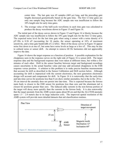
Compact Low-Cost Ultra-Wideband EMI SensorSERDP MR-2105center time. The last gate was 45 samples (469 s) long, and the preceding gatelengths decreased geometrically based on the gate time. The first 12 time gates areonly one sample long because the ADC sample rate was insufficient to follow the10% length rule for early time gates.5. The average value of the half-cycle waveforms in each time gate was calculated toproduce the decay waveforms shown in Figure 15 and Figure 16.The initial part of the decay curves shown in Figure 15 and Figure 16 is blocky because theADC sample rate was insufficient to follow the 10% gate length rule for the first 12 time gates.The expected noise level for the last time gate when using a sensor with a noise density of 6pT/Hz is 0.56 nT (accounting for 10 stacks, the sensor operating at 16% of maximumsensitivity, and a time gate bandwidth of 2.2 kHz). Most of the decay curves in Figure 16 appearnoise free down to at one nT, but some have noise levels as large as a few nT. This may be dueto cultural noise or sensor drift. An attempt to remove 60 Hz harmonics did not appreciablyimprove the data.Figure 16 shows the target response as a function of position. A possible explanation for thechoppiness seen in the response curves on the right side of Figure 16 is sensor drift. The targetresponse data and the background response data were taken at different times, but within a fewminutes of each other. Drift in the sensor baseline between target and background recordingscauses uncertainty in the actual baseline value and may add unwanted choppiness in the EMIresponse versus position. A solution to this problem is to make precise baseline measurementsthat account for drift as described in the Sensor Calibration and Drift section below. Althoughaccounting for drift is impractical with the current electronics, the next generation electronicsdesign will account and compensate for drift. In Figure 16 it is noteworthy that the early-timeand late-time curves for positions less than 0 cm show similar anomalies, but in the in the -20 to -30 cm interval the anomaly does not persist into late-time. This is expected because the ferrousmain body is closest to the EMI sensor for positions less than zero and the aluminum tail isclosest for positions greater than zero. The induced eddy currents in the non-ferrous portion ofthe target will decay more quickly than the currents in the ferrous body. It is also noteworthythat the target anomaly from the AMR system spans about 80 cm and that the ALLTEM anomalyspans 1.5 – 2.0 meters due to its large induction coils. The improved spatial resolution of theAMR system will provide more detailed datasets that aid classification routines.Figure 17. Illustration of magnetometer test setup.17