Continuous Cooling Transformation (CCT) Diagrams

Continuous Cooling Transformation (CCT)
Diagrams
R. Manna
Assistant Professor
Centre of Advanced Study
Department of Metallurgical Engineering
Institute of Technology, Banaras Hindu University
Varanasi-221 005, India
rmanna.met@itbhu.ac.in
Tata Steel-TRAERF Faculty Fellowship Visiting Scholar
Department of Materials Science and Metallurgy
University of Cambridge, Pembroke Street, Cambridge, CB2 3QZ
rm659@cam.ac.uk

Continuous cooling transformation (CCT) diagram
Definition: Stability of phases during continuous
cooling of austenite
There are two types of CCT diagrams
I) Plot of (for each type of transformation) transformation start,
specific fraction of transformation and transformation finish
temperature against transformation time on each cooling curve
II) Plot of (for each type of transformation) transformation start,
specific fraction of transformation and transformation finish
temperature against cooling rate or bar diameter for each type of
cooling medium 2

Determination of CCT diagram type I
CCT diagrams are determined by measuring some physical
properties during continuous cooling. Normally these are
specific volume and magnetic permeability. However, the
majority of the work has been done through specific volume
change by dilatometric method. This method is supplemented
by metallography and hardness measurement.
In dilatometry the test sample (Fig. 1) is austenitised in a
specially designed furnace (Fig. 2) and then controlled cooled.
Sample dilation is measured by dial gauge/sensor. Slowest
cooling is controlled by furnace cooling but higher cooling rate
can be controlled by gas quenching.
3

Fig. 1: Sample and fixtures for
dilatometric measurements
Fig. 2 : Dilatometer equipment
4

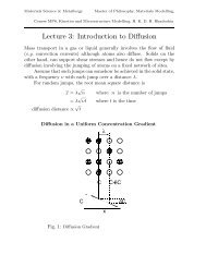
Temperature
Cooling data are plotted as temperature versus time (Fig. 3).
Dilation is recorded against temperature (Fig. 4). Any slope
change indicates phase transformation. Fraction of
transformation roughly can be calculated based on the dilation
data as explained below.
I
II
Time
III
IV
Fig. 3: Schematic cooling curves
V
Dilation
For a cooling
schedule
d
c
T F
Temperature
b
T S
Fig. 4: Dilation-temperature plot
5
for a cooling curve
X
Y
Z
T
a

In Fig. 3 curves I to V indicate cooling curves at higher
cooling rate to lower cooling rate respectively. Fig. 4 gives the
dilation at different temperatures for a given cooling
rate/schedule. In general slope of dilation curve remains
unchanged while amount of phase or the relative amount of
phases in a phase mixture does not change during cooling (or
heating) however sample shrink or expand i.e. dilation takes
place purely due to thermal specific volume change because of
change in temperature. Therefore in Fig. 4 dilation from a to b
is due to specific volume change of high temperature phase
austenite. But at T S slope of the curve changes. Therefore
transformation starts at T S. Again slope of the curve from c to
d is constant but is different from the slope of the curve from a
to b. This indicates there is no phase transformation between
the temperature from c to d but the phase/phase mixture is
different from the phase at a to b.
6

Slope of the dilation curve from b to c is variable with
temperature. This indicates the change in relative amount of phase
due to cooling. The expansion is due to the formation of low
density phase(s). Some part of dilation is compensated by purely
thermal change due to cooling. Therefore dilation curve takes
complex shape. i.e first slope reduces and reaches to a minimum
value and then increases to the characteristic value of the phase
mixture at c.
Therefore phase transformation start at b i.e. at temperature T S
and transformation ends or finishes at c or temperature T F. The
nature of transformation has to be determined by metallography.
When austenite fully transforms to a single product then amount
of transformation is directly proportional to the relative change in
length. For a mixture of products the percentage of austenite
transformed may not be strictly proportional to change in length,
however, it is reasonable and generally is being used.
7

Cumulative percentage of transformation at in between
temperature T is equal to YZ/XZ*100 where X, Y and Z are
intersection point of temperature T line to extended constant
slope curve of austenite (ba), transformation curve (bc) and
extended constant slope curve of low temperature phase (cd)
respectively.
So at each cooling rate transformation start and finish
temperature and transformation temperature for specific
amount (10 %, 20%, 30% etc.) can also be determined. For
every type of transformation, locus of start points,
isopercentage points and finish points give the transformation
start line, isopercentage lines and finish line respectively and
that result CCT diagram. Normally at the end of each cooling
curve hardness value of resultant product at room temperature
and type of phases obtained are shown.
8

• Fig. 5 shows the five different cooling curves a to e employed
to a hypoeutectoid steel. Fig. 5(a) to (e) show the type of
corresponding dilatometric plots drawn against dilation versus
temperature. Fig. 6 shows the corresponding transformation
temperature and time in a temperature versus log time plot
against each corresponding cooling rate. At the end of each
cooling rate curve normally hardness value and type of phases
obtained at room temperature are shown. Symbols F, P, B, M
stand for ferrite, pearlite, bainite and martensite respectively.
Subscripts ‘S and ‘F’ stand for reaction start and reaction
finish respectively. In cooling ‘a’ schedule martensite starts at
M S and finishes at M F and therefore 100% martensite results.
While in cooling schedule ‘b’ bainite starts at B S but reaction
does not complete and retained austenite enriched in carbon
transforms at lower M S but completes at lower M F. Cooling
schedule ‘b’ results bainite and martensite.
9

Dilation
Dilation
Temperature
a
b c d e
Time
temperature
M F
b
a
M F
M S
M S
B S
Temperature
dilation
dilation
dilation
M F
c
e
M S
B S
F F
F S
Temperature
d
B F
F F
B S
Temperature
P F
Temperature
F S
P S
F S
Temperature
Ae 3
Ae 1
a b
M S
M F
c d
B S
F S
B F
P S
M
HV
M+B
HV
F+B F+B F+P
HV HV
HV
Log time
Fig. 5: Schematic dilatometric plots for five different cooling rates where F, Fig. 6: Schematic CCT diagram constructed
P, B and M stands for ferrite, pearlite, bainite and martensite respectively from data of Fig 3(for the hypoeutectoid
and subscript S and F stands for transformation start and transformation steel). Dotted line is 25% of total
finish for respective products for a hypoeutectoid steel
transformation.
e
10

In cooling schedule ‘c’ ferrite starts at F S and finishes at F F.
Quantity of ferrite is about 15% but rest of austenite enriched
in carbon transforms to bainite at B S and just finishes at B F.
Therefore cooling ‘c’ results ferrite and bainite at room
temperature. Similarly cooling schedule ‘d’ results increased
ferrite and rest bainite. During cooling schedule ‘e’ ferrite start
at F S and pearlite starts at P S but pearlite reaction finishes at P F.
Therefore cooling schedule ‘e’ results increased ferrite and rest
pearlite. The locus of all start points and finish points result the
CCT diagram. This diagram is not a unique diagram like TTT
diagram for a material. It depends on type of cooling. This
diagram can predict phase transformation information if
similar cooling curves had been used during its determination
or if equivalent cooling schedule are used during process of
production.
11

The two cooling curves are considered equivalent if
(i) the times to cool from A e3 to 500°C are same.
(ii) the times to cool from A e3 to a temperature halfway
between Ae 3 and room temperature , are same.
(iii) the cooling rates are same.
(iv) the instant cooling rates at 700°C are same.
Therefore to make it useful different types of CCT diagrams
need to be made following any one of the above schedule that
matches with heat treatment cooling schedule.
12

End-quench test method for type I CCT diagram
A number of Jominy end quench samples are first end- quenched
(Fig.7) for a series of different times and then each of them (whole
sample) is quenched by complete immersion in water to freeze the
already transformed structures. Cooling curves are generated putting
thermocouple at different locations and recording temperature
against cooling time during end quenching. Microstructures at the
point where cooling curves are known, are subsequently examined
and measured by quantitative metallography. Hardness
measurement is done at each investigated point. Based on
metallographic information on investigated point the transformation
start and finish temperature and time are determined. The
transformation temperature and time are also determined for specific
amount of transformation. These are located on cooling curves
plotted in a temperature versus time diagram. The locus of
transformation start, finish or specific percentage of transformation
generate CCT diagram (Fig. 8). 13

2½”(64 mm)
Free height
of water jet
Nozzle
1⅛”(29 mm)
diameter
1⅓ 2”(26.2 mm)
1”(25.4 mm)
diameter
Water
umbrella
½”(12.7 mm)
½”(12.7 mm) diameter
⅛”(3.2 mm)
½”(12.7 mm)
4”(102 mm)
long
Fig 7(a): Jominy sample with fixture and water jet
14

c
Fig.7: Figures show (b) experimental set up, (c ) furnace for
austenitisation, (d) end quenching process. Courtesy of
DOITPoMS of Cambridge University.
b
d
15

Temperature
A e1
t0 t’ 0
Hardness, HRC
F
EDC
F E D
Distance from quench end
a
B
b c d
C
M S, Martensite start temperature
B
M50,50% Martensite
Metastable austenite +martensite
MF, Martensite finish temperature
Martensite Martensite
Pearlite+Martensite
Fine pearlite
pearlite Coarse
pearlite
Log time
A
Jominy
sample
A
t o=Minimum
incubation period at
the nose of the TTT
diagram,
t’ o=minimum incubation
period at the nose of the
CCT diagram
Fig. 8: CCT
diagram ( )
projected on
TTT diagram
( ) of eutectoid
steel
16

Fig. 7. shows the Jominy test set up and Fig. 6 shows a schematic
CCT diagram. CCT diagram is projected on corresponding TTT
diagram.
A, B, C, D, E, F are six different locations on the Jominy sample
shown at Fig.8 that gives six different cooling rates. The cooling
rates A, B, C, D, E, F are in increasing order. The corresponding
cooling curves are shown on the temperature log time plot. At the
end of the cooling curve phases are shown at room temperature.
Variation in hardness with distance from Jominy end is also
shown in the diagram.
For cooling curve B, at T 1 temperature minimum t 1 timing is
required to nucleate pearlite as per TTT diagram in Fig. 8. But
material has spent t 1 timing at higher than T 1 temperature in
case of continuous cooling and incubation period at higher
temperature is much more than t 1. The nucleation condition
under continuous cooling can be explained by the concept of
progressive nucleation theory of Scheil. 17

Scheil’s concept of fractional nucleation/progressive
nucleation
Scheil presented a method for calculating the transformation
temperature at which transformation begins during continuous
cooling. The method considers that (1) continuous cooling occurs
through a series of isothermal steps and the time spent at each of
these steps depends on the rate of cooling. The difference between
successive isothermal steps can be considered to approach zero.
(2) The transformation at a temperature is not independent to cooling
above it.
(3) Incubation for the transformation occurs progressively as the
steel cools and at each isothermal step the incubation of
transformation can be expressed as the ratio of cooling time for the
temperature interval to the incubation period given by TTT diagram.
This ratio is called the fractional nucleation time.
18

Scheil and others suggested that the fractional nucleation time are
additive and that transformation begins when the sum of such
fractional nucleation time attains the value of unity.
The criteria for transformation can be expressed
Δt 1/Z 1+Δt 2/Z 2+Δt 3/Z 3+…….+Δt n/Z n=1
Where Δt n is the time of isothermal hold at Temperature T n where
incubation period is Z n. This is called additive reaction rule of
Scheil (1935). The reactions for which the additive rule is justifiied
are called isokinetic, implying that the fraction transform at any
temperature depends only on time and a single function of
temperature. This is experimentally verified by Krainer for
pearlitic transformation.
19

Therefore though nucleation has progressed to some fraction of the
event but time is not sufficient for pearlite nucleation at a. If time is
allowed in continuous cooling while summation of fractional
nucleation time becomes unity (at b), pearlite is to nucleate but by
that time temperature drops down as it is continuously cooling.
This concept of progressive nucleation is not strictly valid for
bainite transformation where austenite get enriched with carbon at
higher temperature. As transformation at higher temperature
enriches the austenite by carbon, the transformation characteristic
changes. i.e. transformation slows down at lower temperature.
By continuous cooling transformation temperature moves towards
down and incubation moves toward right. Similar is the case for
pearlite finish temperature and time. Pearlitic region takes the
shape as shown in the diagram. The bainitic region moves so right
that entire region is sheltered by the pearlitic curve.
20

So there is no chance of bainitic tranformation in eutectoid
plain carbon steel under continuous cooling condition. There is
untransformed region where earlier was bainitic region. Under
such circumtances split transformation occurs. However
martensitic region remain unaffected.
Various cooling rates give various combination of phases.
Cooling A indicates very slow cooling rate equivalent to
furnace cooling of full annealing process and that results
coarse pearlite. Cooling B is faster cooling can be obtained
by air cooling. This type of cooling can be obtained by
normalising and that results finer pearlite. Cooling C: just
touches the finishing end of nose that gives fully fine pearlite.
Cooling D is faster cooling that can be obtained by oil
quenching. This is a hardening heat treatment process and that
produces fine pearlite and untransformed austenite transforms
to martensite below M S.
21

Cooling curve E just touches the nose of CCT diagram and that
produces almost fully martensite.
Cooling curve F avoid nose of C curve in CCT but touches the
nose of TTT gives entirely martensite. Notice the critical cooling
rate to avoid nose of CCT diagram i.e. diffusional
transformations is lower than that to TTT diagram.
22

General features of CCT diagrams
1. CCT diagram depends on composition of steel, nature of cooling,
austenite grain size, extent of austenite homogenising, as well as
austenitising temperature and time.
2. Similar to TTT diagrams there are different regions for different
transformation (i.e. cementite/ferrite, pearlite, bainite and
martensite). There are transformation start and transformation finish
line and isopercentage lines. However depending on factors
mentioned earlier some of the transformation may be absent or some
transformation may be incomplete.
3. In general for ferrite, pearlite and bainite transformation start and
finish temperature moves towards lower temperature and
transformation time towards higher timing in comparison to
isothermal transformation. Transformation curve moves down and
right.
23

4. The bainite reaction can be sufficiently retarded such that
transformation takes shelter completely under pearlitic transformation
in case of eutectoid plain carbon steel and therefore bainite region
vanishes. However in other steel it may be partially sheltered.
Therefore bainitic region observed in non eutectoid plain carbon steel
or alloy steels.
5. C curves nose move to lower temperature and longer time. So actual
critical cooling rate required to avoid diffusional transformation
during continuous cooling is less than as prescribed by TTT diagram.
Actual hardenability is higher than that predicted by TTT.
6. M S temperature is unaffected by the conventional cooling
rate,however, it can be lowered at lower cooling rate if cooling curves
such that austenite enriches with carbon due to bainite or ferrite
formation (in hypoeutectoid steel). On the other hand M S can go up
for lower cooling rate such that austenite become lean in carbon due
to carbide separation (in hypereutectiod steel). 24

7. Large variety of microstructure like ferrite/cementite/carbide
+pearlite+bainite+martensite can be obtained in suitable cooling
rate. It is not feasible or limited in case of isothermal
transformation.
25

Determination of type II CCT diagram
This procedure was developed by Atkins. In this process round
samples of different diameters were quenched in three different
media air, oil and water. The cooling curves were recorded at the
centre of each bar. Later these cooling curves were simulated in
dilatometer test in order to identify the transformation
temperature, microstructure and hardness. The transformation
information is plotted against temperature and bar diameter
cooled in specific medium. These are bar diameter cooled in air,
quenched in oil and quenched in water. A scale cooling rate
(usually at 700°C) in °C/min is added.
At the bottom of the same diagram another plot is added for
hardness (in HRC) and with same cooling rate axis/bardiameter.
These diagrams have to be read along vertical lines (from top to
bottom), denoting different cooling rates. Fig. 9 shows a
schematic CCT diagram for hypoeutectoid plain carbon steel.
26

Hardness, HV
Temperature, °C
M s
M 50
M 90
M f
Bar diameter, in mm
Cooling rate at 700°C, °C per min
Oil quench
Water quench
Hardness after transformation at room temperature
Air cooled
Hardness, HRC
0% 50%
90%
100%
Fig. 9: CCT
diagram for
hypoeutectoid
steel
27

Conversion of TTT to CCT diagram, Scheil’s
method (1935)
Scheil’s method is based on the assumption that the continuous
cooling curve is a combination of sufficiently large number of
isothermal reaction steps. Incubation for the transformation
occurs progressively as the steel continuously cools.
Transformation begins when the sum of fractional nucleation
time attains the value of unity.
The criteria for transformation can be expressed
Δt 1/Z 1+Δt 2/Z 2+Δt 3/Z 3+…….+Δt n/Z n=1
Where Δt n is the time of isothermal hold at temperature T n
where incubation period is Z n. The rule can be justified if
reaction rate solely depends on volume fraction and
temperature.
28

Conversion of TTT to CCT, Grange and Kiefer Method
(1941)
During continuous cooling along a given cooling curve which
intercepts the TTT start curve at temperature T 1, the
transformation will start at temperature T 2, such that the time of
cooling between T 1 and T 2 is equal to the time for the start of
transformation during isothermal holding at temperature T 3=
(T 1+T 2)/2 (as shown in Fig. 10).
t 3=t 2-t 1
Similar rule can be applied for a isopercentage curve and finish
curves.
Assumptions are not strictly valid, however, the method gives
reasonable result. The method is particularly suitable for ferritepearlite
region
29

Temperature
Ae 3
T1 T3 T2 t 3 t 1 t 2
Log time
T 3=(T 1+T 2)/2
and t 3=t 2-t 1
or t 2=(t 1+t 3)/2
Fig. 10: Graphic method of converting TTT diagram to CCT diagram
[Grange and Kiefer method]
30

Conversion of TTT to CCT, Avrami method (1939)
Let τ TTT(T) be time required to obtain a given percentage of
transformation, X at temperature T during isothermal
transformation.
Then time required(τ CCT) to obtain the same percentage of
transformation, X, on continuous cooling at T CCT is given by the
condition
X=∫ T
Ae3 CCT dX= ∫ TCCT Ae3 dX/dt.dt= ∫ TCCT g-dt-------1
Ae3
g-=time average transformation rate (at any temperature T)=X/τIT(T). Substituting this in equation 1
We get ∫ TCCT Ae3 dt/ τTTT(T) =1--------2,
By rewriting equation 2 we get
∫ Ae3
T CCT dT/(τ TTT(T) dT/dt)=1----------3
Both these integrals are called Avrami integral. Any one of these
integrals has to be evaluated for each cooling curve to get the τ CCT at
T CCT 31

Conversion of CCT to TTT diagram, Kirkaldy and
Sharma method (1982)
Let τ CCT(T CCT) be the time required to obtain a given
percentage of transformation, X at temperature T CCT during
continuous cooling. If it is assumed that CCT diagram was
constructed using constant cooling rate(linear cooling),
Then
dT/dt=-(A e3-T CCT)/(τ CCT(T CCT)----4
Substituting equation 4 in equation 3, cross multiplying and
differentiating with respect to T CCT
We get
τ TTT(T CCT)=1/(d/dT CCT[(A e3-T CCT)/τ CCT(T CCT)])---5
Where τ TTT is the time required for the given percentage
transformation, X, when carried out isothermally at T CCT.
32

While rate of cooling is not constant but cooling rate can be
expressed analytically or empirically as
dT/dt=f 1(x)f 2(T)=f 1(T CCT)f 2(T) ---6 (Exp: Jominy cooling
curve can be expressed in this form)
where x is the distance from the surface of a continuouly cooled
sample.
Substituting equation 6 in equation 3, cross multiplying and
differentiating
We get
τ TTT (T CCT)=1/(f 2(T CCT) df 1/dT CCT)-----7
Equation 5 or 7 can be used for the conversion of CCT diagram to
TTT diagram depending on constant cooling rate or case of cooling
rate that can be expressed in analytical or empirical form.
Jominy cooling curves can be expressed in equation 6 form and the
using equation 7, CCT diagram can be converted to TTT diagram.
33