Thesis (PDF) - Signal & Image Processing Lab

More documents

Recommendations

Info

32 CHAPTER 2. THEORETICAL BACKGROUND Keshet also defines in [16] the notion of boundary topographic distance (BTD) of a pixel x of a bounded image f, as the topographic distance between x and the boundary of f. That is, the BTD of x is the least topographic distance between x and any point on the boundary of f. The BTD function, BTf, is the mapping from each pixel x to its BTD, BTf(x). 2.5.2 An extension of boundary topographic distance defini- tion The notion of BTD, defined by Keshet, can be easily extended, allowing the boundary of the image f to be any connected flat zone of f. The notion of flat zone is discussed in section 2.2. In some cases, a boundary of an image isn’t the best starting point for topographic distance calculation, because it is arbitrary set by the properties and position of the camera used to take the picture. When choosing another flat zone, as a reference for the topographic distance, the choice can be more meaningful and suited for the problem to be solved. For instance, in some applications it can be useful to define the boundary as the largest flat zone of the image. Another example is shown in Fig. 2.9. In this example a root flat zone is chosen to a be a symmetric center of the image - the circle center. 2.5.3 Boundary Topographic Variation (BTV) Transform Let πf(x) be a connected path linking the boundary of an image f to a pixel x and ˆπf(x) be one such path, with least topographic distance between x and the boundary. The topographic distance (total variation) on ˆπf(x) is exactly BTf(x) and ˆπf(x) is called a minimal-BTD path for x. There may be more than one minimal-BTD path for a given point x. Assume that a minimal-BTD path is associated with an alternating sequence (AS). The AS describes the “ups and downs” that occur on that path. These “ups and downs” are called path variation. For instance, consider a grayscale image f, and suppose that a minimal-BTD path ˆπf(x) from the boundary to a pixel x has the following function values: f(ˆπf(x)) = (0, 2, 6, 9, 8, 8, 5, 1, 3, 7, 7, 4, 5). (2.19)
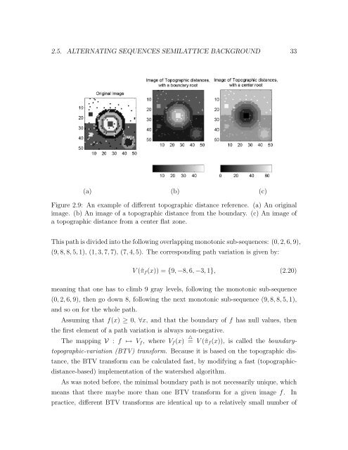
2.5. ALTERNATING SEQUENCES SEMILATTICE BACKGROUND 33 (a) (b) (c) Figure 2.9: An example of different topographic distance reference. (a) An original image. (b) An image of a topographic distance from the boundary. (c) An image of a topographic distance from a center flat zone. This path is divided into the following overlapping monotonic sub-sequences: (0, 2, 6, 9), (9, 8, 8, 5, 1), (1, 3, 7, 7), (7, 4, 5). The corresponding path variation is given by: V (ˆπf(x)) = {9, −8, 6, −3, 1}, (2.20) meaning that one has to climb 9 gray levels, following the monotonic sub-sequence (0, 2, 6, 9), then go down 8, following the next monotonic sub-sequence (9, 8, 8, 5, 1), and so on for the whole path. Assuming that f(x) ≥ 0, ∀x, and that the boundary of f has null values, then the first element of a path variation is always non-negative. The mapping V : f ↦→ Vf, where Vf(x) △ = V (ˆπf(x)), is called the boundary- topographic-variation (BTV) transform. Because it is based on the topographic distance, the BTV transform can be calculated fast, by modifying a fast (topographic- distance-based) implementation of the watershed algorithm. As was noted before, the minimal boundary path is not necessarily unique, which means that there maybe more than one BTV transform for a given image f. In practice, different BTV transforms are identical up to a relatively small number of
Page 1 and 2: SELF-DUAL MORPHOLOGICAL OPERATORS B
Page 3 and 4: The Research Thesis was done under
Page 5 and 6: iv CONTENTS 3 Implementation of BTV
Page 7 and 8: List of Tables 2.1 The BTV transfor
Page 9 and 10: viii LIST OF FIGURES 2.9 An example
Page 11 and 12: x LIST OF FIGURES 4.17 A Simba imag
Page 13 and 14: xii LIST OF FIGURES 6.20 A Lena ima
Page 15 and 16: Abstract This research addresses a
Page 18 and 19: 4 List of Abbreviations and Symbols
Page 20 and 21: 6 CHAPTER 1. INTRODUCTION the image
Page 22 and 23: 8 CHAPTER 1. INTRODUCTION disadvant
Page 24 and 25: 10 CHAPTER 1. INTRODUCTION 3. A gen
Page 26 and 27: Chapter 2 Theoretical Background 2.
Page 28 and 29: 14 CHAPTER 2. THEORETICAL BACKGROUN
Page 52 and 53: 38 CHAPTER 3. IMPLEMENTATION OF BTV
Page 58 and 59: Chapter 4 The “trench” problem
Page 60 and 61: 46CHAPTER 4. THE “TRENCH” PROBL
Page 76 and 77: Chapter 5 Tree Semilattices In this
Page 78 and 79: 64 CHAPTER 5. TREE SEMILATTICES sec
Page 80 and 81: 66 CHAPTER 5. TREE SEMILATTICES Fig
Page 82 and 83: 68 CHAPTER 5. TREE SEMILATTICES tre
Page 84 and 85: 70 CHAPTER 5. TREE SEMILATTICES If
Page 86 and 87: 72 CHAPTER 5. TREE SEMILATTICES sam
Page 88 and 89: 74 CHAPTER 5. TREE SEMILATTICES rep
Page 90 and 91: 76 CHAPTER 6. EXTREMA-WATERSHED TRE
Page 96 and 97:
82 CHAPTER 6. EXTREMA-WATERSHED TRE
Page 98 and 99:
Page 100 and 101:
Page 102 and 103:
Page 104 and 105:
Page 106 and 107:
Page 108 and 109:
Page 110 and 111:
Page 112 and 113:
Page 114 and 115:
100 CHAPTER 6. EXTREMA-WATERSHED TR
Page 116 and 117:
Page 118 and 119:
Page 120 and 121:
Page 122 and 123:
Page 124 and 125:
Page 126 and 127:
Chapter 7 Conclusions and further r
Page 128 and 129:
Appendix A 114
Page 130 and 131:
Bibliography [1] J. Serra, Image An
Page 132:
118 BIBLIOGRAPHY [21] Renato Keshet
show all

Thesis (PDF) - Signal & Image Processing Lab

Create successful ePaper yourself

Delete template?

Save as template?